Article

Investigating the Causal Relationships among Carbon Emissions, Economic Growth, and Life Expectancy in Turkey: Evidence from Time and Frequency Domain Causality Techniques

by
Husam Rjoub
1,*,
Jamiu Adetola Odugbesan
2,
Tomiwa Sunday Adebayo
2 and
Wing-Keung Wong
3
1
Department of Accounting and Finance, Faculty of Economics and Administrative Sciences, Cyprus International University, Mersin 10, 99040 Haspolat, Turkey
2
Department of Business Administration, Faculty of Economics and Administrative Sciences, Cyprus International University, Mersin 10, 99040 Haspolat, Turkey
3
Department of Finance, Fintech & Blockchain Research Center, and Big Data Re-search Center, Asia University, Taichung 41354, Taiwan
*
Author to whom correspondence should be addressed.
Sustainability 2021, 13(5), 2924; https://doi.org/10.3390/su13052924
Submission received: 18 February 2021 / Revised: 1 March 2021 / Accepted: 2 March 2021 / Published: 8 March 2021

Abstract

:
It is not a gainsaying that challenges to both healthy living and the environment are the result of deteriorating environmental quality with the attendant effect on environmental sustainability. To provide a solution to the issue, our study uses long time-series data from 1960 to 2018, and employs an overlapping generational model, the Bayer–Hanck cointegration test, wavelet coherence, Fourier Toda–Yamamoto, and Breitung–Candelon frequency-domain spectral causality tests to investigate the causal relationships among carbon emissions (CO2), economic growth (GDP), and life expectancy (LE) in Turkey. Different from the literature, we find a positive co-movement between life expectancy and CO2 and a positive correlation between LE and GDP at different scales; CO2 has a causal relationship with LE and a bidirectional causal relationship between LE and GDP, as well as short, medium, and long-run causal relationships with LE; GDP has medium and long-run causal relationships with LE, and LE has short, medium, and long-run causal relationships with GDP. Our findings guide policymakers on their policy decision-making that will address the energy consumption, environmental degradation, human health, environmental hazards, and allocation to science and technology in Turkey with the aim of ensuring overall sustainable development.

1. Introduction

The challenges of healthy living along with the increasing threat of global warming all around the globe are the result of the increasing deterioration in environmental quality across the world [1]. Owing to the increasing attention of scholars towards global warming and environmental challenges, the economic policymakers, and other stakeholders are getting more interested in the relationship between environmental consequences and health outcomes [2,3,4]. Air pollution has been a serious concern to the environmentalist and policymakers, especially the carbon emissions (CO2) from the rapid industrialization and the use of energy, and this has been recognized as one of the determinants of health problems around the world [1], as well as a major factor capable of affecting the achievement of environmental sustainability [5,6,7]. Notably, one of the main contributors to global climate change has been CO2, which has received considerable attention from policymakers, as well as being the main focus in most of the research across different fields of study [1,5,6,7,8].
From an economic perspective, CO2 is considered as the logical consequence of industrial activities, which, although they create added value, are polluting; thus, CO2 emissions are seen as a guaranteed effect of significant economic growth. Meanwhile, most studies have generally focused on the trade-off between economic growth and CO2 emissions, but the effects of environmental pollution on human health that affect society in terms of life expectancy are substantial, as well as its effect on achieving environmental sustainability [7]. Meanwhile, Mariani et al. [9] opined that the nexus between life expectancy and environmental quality could go the other way round. Life expectancy is a measure of the length of life expected of an individual to be lived at birth (Agbanike et al. [2]). It is considered in the literature as significant nations’ health condition and individual well-being indicator [3,4,10]. Alam et al. [11] and Shahbaz et al. [12] noted that since individuals make up a nation, improving life expectancy is a significant and necessary condition that is required for guaranteeing sustainable economic development. The reflection of life expectancy in the social, economic, and environmental condition of a nation is demonstrated in some studies [2,12,13]; hence, the causal relationship among economic, social, and environmental factors and life expectancy in a given country have become a very important issue among policymakers, whereas, the empirical studies investigating the relationship between economic growth and life expectancy [2,14], and carbon emissions and life expectancy [1,15] have been mixed. In addition, the studies investigating the relationship among economic growth, carbon emissions, and life expectancy together are relatively rare and recent, especially in Turkey. Hence, this study aims to fill this identified gap in the existing literature by investigating the causal relationship among carbon emissions, economic growth, and life expectancy in Turkey.
This study focuses on Turkey, owing to its rise and fall in economic growth [World Bank, 2020], its ever-increasing carbon emissions [16], and the life expectancy of 77.44 years as of 2018—above the world average of 72.6 years in the same year [17]. Turkey is considered to be a less developed country with a USD 754.41 billion GDP and USD 9042.49 per capita GDP as of 2019 [17]. Turkey as a less developed country has boosted its energy needs in all sectors and is thus characterized as a rapid economic growth country with an increased rate of rigid energy demand and urbanization, and these in no small measure contribute to the increasing carbon emissions in the country (see Bilgen [18]). The developments in Turkey have resulted in the economy growing by 1.15% in 1960 and 7.47% in 2017 but plummeted to 0.877% in 2019. Such rapid economic growth between 1960 to 2017 has been accompanying by the “CO2 increase from 0.61 metric tons per capita in 1960 to 4.67 metric tons per capita in 2016 accounting for a 636% rise in metric tons per capita in the country as of 2016” [17], even though, during the period under observation, the life expectancy at birth improved from 45.37 years in 1960 to 77.44 years in 2018, which is above the global average of 72.6 years [17].
According to “Turkiye Istatistik Kurumu” (TUIK) [19], the energy consumption in Turkey generates greenhouse gas (GHG), which is mostly carbon emissions, having a share of over 80% of total GHG in the country. Turkey received candidate status of EU membership in 1999 after fulfilling the acquis, among which was its environmental issues; however, Turkey has been found to be the third-highest CO2 emissions-generating country among EU members [7,16], and this definitely will have implications for the people’s health and/or life expectancy, which, in turn, has an effect on economic growth, and on carbon emissions. It is then imperative to investigate the causal relationship between carbon emissions, economic growth, and the life expectancy in the country, so as to guide the policymakers in Turkey to redirect the “national environmental policies”, especially policies related to mitigating the increase in CO2 emissions. Thus, this study investigates the causal relationship between CO2 emissions and the life expectancy of Turkey’s population, using some new econometric techniques to enhance the validity of our findings.
In this paper, we use the long time-series data from 1960 to 2018, employ the overlapping generational model to provide a theoretical background for our study, employ ADF, PP, Zivot–Andrews, and Lee–Strazicich unit root tests to test for unit roots, use the Bayer–Hanck cointegration test to conduct a robust cointegration analysis, and employ both time and frequency-domain causality tests to investigate the causal relationships among economic growth, life expectancy, and the CO2 emissions in Turkey. Different from the existing literature, using wavelet coherence techniques, we find positive co-movement between life expectancy and CO2 emissions and positive correlations between life expectancy and economic growth at different scales. Using the Fourier Toda–Yamamoto causality test, we find that CO2 has a causal relationship with life expectancy, establishing a bidirectional relationship between life expectancy and economic growth. Employing the Breitung–Candelon frequency-domain spectral causality test, we found that CO2 has short-, medium-, and long-run causal relationships with life expectancy; economic growth has medium- and long-run causal relationships with life expectancy; and life expectancy has short-, medium-, and long-run causal relationships with economic growth. Generally, our study provides new empirical evidence on the causal relationships among economic growth, CO2, and life expectancy in Turkey. Our findings could be used for policymakers on their policymaking on sustainability, energy consumption, environmental degradation, human health, environmental hazards, allocation to science and technology, and pollution. Additionally, to the best of the author’s understanding, most studies that have examined these interconnections used time-domain econometric techniques such as the fully-modified ordinary least squares (FMOLS) and dynamic ordinary least squares (DOLS) methods, in addition to the canonical cointegration regression (CCR), autoregressive distributed lag (ARDL), vector error correction model (VECM), and many more. Thus, the present study fills the gaps in prior studies by utilizing the wavelet methodologies to capture relationships at different frequencies and different periods. Moreover, the wavelet approach is used because it offers information on both the phase and amplitude, which are crucial to examine dissimilar time-series synchronization and the interconnection of these economic variables over time.
The remainder of the study is structured as follows: Section 2 consists of the review of related studies, Section 3 presents the empirical methodology, Section 4 presents the empirical findings and discussions, and Section 5 rounds up the study with the conclusions.

2. Literature Review and Hypotheses Development

2.1. Literature Review

The exploration of the causal relationship between life expectancy and economic growth has been conducted by many scholars in different regions across different periods utilizing single-country and panel studies. However, there is no consensus on the findings with mostly three strands observed in the literature, exhibiting negative, positive, and non-linear relationships between them. Among the recent studies on this subject was a study conducted in the African economy to investigate the relationship of variables such as population, democracy, economic growth, and life expectancy; the study found a positive and significant nexus between economic growth and life expectancy (Biyase and Malesa [10]). The study employed two-stage least square and observed data from 1985 to 2017. Another study investigated the dynamic relationship between economic growth and life expectancy in Pakistan applying the ARDL bounds test and found a positive influence of economic growth on life expectancy (Wang et al. [14]). In addition, the study of Govdeli et al. [20] investigated E7 countries using data from 1992 to 2016 and employed a causality test and found a significant nexus between economic growth and life expectancy. A similar finding was established by Shahbaz et al. [21], who did a similar study in sub-Saharan Africa by employing a parametric cointegration test and found a positive and significant relationship between the two variables.
Moreover, a non-linear causality was employed by Shahbaz et al. [12] to investigate the scenario in Pakistan. The study suggested that sustainability is most possible in the countries with the best health infrastructure and economic growth, and also that the governments of the countries have a crucial role to play in ensuring the increase in the life expectancy level of their people. Furthermore, a positive impact of life expectancy on economic growth was demonstrated in the study by Biyase and Malesa [10], which was conducted in 10 Southern African countries using data from 1985 to 2017 and applied a two-stage least square method, while a bidirectional relationship between the two variables was found in the study by He and Li [15] which used 65 countries. Meanwhile, the study by Sirag et al. [22] found that life expectancy plays a significant role in economic development but suggested that it is up to a certain threshold. The finding is consistent with Yakita [23] who revealed that an increase in longevity increases the balance of the growth rate. Several studies agree with the position that life expectancy affects economic growth via the increase of the investment in capital [15,24].
A negative link between economic growth and life expectancy was reported in some studies. For instance, the study of Acemoglu and Johnson [25], conducted in 47 countries under the category of developed and less developed countries of the world, revealed a negative and insignificant relationship between the two variables. This finding was corroborated by Leung and Wang [26] who examined the endogenous nexus between life expectancy and output in a neoclassical growth model and found that an increase in life expectancy is negatively related to the income per capita, resulting in a higher dependency ratio.
Another dimension is the non-linear relationship between life expectancy and economic growth. An example is a study by Boucekkine et al. [27] who investigated the influence of life expectancy on economic growth through the overlapping generations (OLG) model with a realistic survival law. The study demonstrates that the growth of GDP per capita is ambiguously affected by an increase in life expectancy, and the influence of life expectancy on GDP per capita growth is positive for low levels of longevity but becomes negative after some level. A similar finding was found by Echevarria [28] who shows in their study that a threshold level exists in the link between life expectancy and output per capita, and their relationship manifests as an inverted U-style pattern. Moreover, the demographic transition was suggested as a mediator in the relationship between life expectancy and economic growth so as to demonstrate the non-linear relationship between the two variables. The study suggests that before a demographic transition, an increase in life expectancy raises the population, but decreases the growth of the population and foster human capital accumulation subsequent to the demographic transition. Similarly, Kunze [29] reveals that increasing life expectancy reduces economic growth under bequests being operative but found the existence of an inverted U-shape nexus between life expectancy and economic growth if bequests were inoperative.
Meanwhile, some studies opined that the consequences of economic growth are often reflected in the environmental deterioration [30,31], which in turn possibly affect health outcomes (Sarkodie et al. [32]). For instance, some studies noted that energy consumption in developing and developed countries are being considered as a significant cause for economic development [33,34]. Meanwhile, Martins et al. [30] and Wang et al. [31] stated that the degradation of the environment and air pollution owing to energy consumption has become a serious and alarming health concern for people around the world. The studies also opined that pollution emanating from the source of energy consumption also affects social and economic causes. The increasing threats of gaseous emissions that are adding to global warming and destructive issues of environmental degradation have brought the issues of both environment and energy economics into eminence in the last few decades. This is evident in the recent study by Sarkodie et al. [32], who found the increase in particulate matters to be a determinant of a reduction in life expectancy. It is also evident from the literature that carbon emissions are considered as the main determinant of environmental deterioration [5,6,7,35,36,37,38] while some studies suggested that it has an effect on health outcomes [2,14,34]. In addition, these emissions in the form of air pollution were stated in some studies to be caused by multiple sources of energy consumption [5,6,7,21,34,39]. Though the studies that investigate the link between environmental degradation and its horrible effects on the level of life expectancy have been scant, some studies demonstrate a positive nexus between environmental degradation and life expectancy in their studies [3,4,40].
The above literature review reveals that there are different findings on the nexus between economic growth and life expectancy on the one hand, and the carbon emissions and life expectancy on the other hand. In addition, the studies employed different methods and samples for both country-specific and panel studies. Meanwhile, the investigation of the causal relationship between economic growth, carbon emissions, and life expectancy, especially in Turkey, has not been previously investigated. Therefore, our study aims to fill the gap. Moreover, in order to reduce the bias of the estimated result and to ensure the validity of our findings, some new econometric techniques were employed for our estimation.

2.2. Theory and Hypotheses

2.2.1. Theory

The trade-off that exists in the nexus between environmental quality and economic growth depends on how people value the future (Clootens [41]). Clootens [41] noted that a rational agent with high life expectancy will place a high value on the future and will be more willing to forego their immediate welfare in favor of future gain. High longevity makes people more sympathetic to the generations to come and/or other future selves [9]. Thus, it is expected that people should invest more in environmental quality to live longer. This argument is demonstrated in the study by Ono and Maeda [42], who introduced the idea of private maintenance based on life expectancy. In another study, it was revealed that under a perfect “annuitization assumption”, a high life expectancy may enhance growth and environmental quality in an OLG framework (Ono and Maeda [42]). On the other hand, environmental quality determines life expectancy. Indeed, the natural environment constitutes significant predictors of life expectancy through several mediums such as natural disasters, climate change, pollution, and so on.
On that note, to investigate the causal relationship among carbon emissions, economic growth, and life expectancy, we consider an overlapping generations model (Pecchenino and Pollard [43], with the incorporation of environmental externalities by John and Pecchenino [44]). Among the assumptions of the models is that a negative aspect of the impact of longevity on growth and the environment is captured by the reduction of unintentional bequests. In addition, a longer life span results in smaller unintentional bequests and therefore reduces the level of the young agents’ wealth. This indicates “a negative income effect on investment in capital and environment, and a positive aspect of longevity is captured by more investment in capital and the environment in preparation for longer life expectancy” (Ono and Maeda [42]). Ono and Maeda [42] demonstrated that, under the extended overlapping generation model, determining the relationship between longevity, economic growth, and the environment is important in the annuity market.
In the study of Mariani et al. [9], two stylized facts about the link between life expectancy and the environment, which are positively correlated, and both bimodally distributed were presented. The study argues that these stylized facts are compatible with—and give support to—the propositions of a two-way causality and the existence of an “environmental poverty trap”, a situation where the life expectancy is considered to be low with a poor environmental quality and a low level of economic growth. Indeed, if the environment is a significant predictor of life expectancy, which is, in turn, a significant determinant for economic growth and environmental expenditure, some economies may be trapped in a vicious circle: “a poor longevity implies low environmental maintenance, which leads to a high level of pollution that in turn keeps life expectancy low” Clootens [41]. Hence, the economy may not be able to develop, since life expectancy is an important factor determining the economy.

2.2.2. Hypotheses

Longevity is usually suggested to be detrimental to both economic growth and the environment due to the old peoples’ dissave, and that reduces investment in capital and the environment. In another dimension, it is, in addition, suggested that longevity is beneficial for economic growth and the environment since young people invest more in the economy and the environment in preparation for their longevity (life expectancy). In order to investigate the causal relationship between the three variables (economic growth, environment, and longevity), we focus on economic growth, environmental externalities as carbon emissions, and longevity as life expectancy with the framework of an overlapping generation model.
This study believes that an important role is being played by the annuity market in the impact of longevity on economic growth and the environmental externalities (carbon emissions), as well as a possible reverse relationship. In this instance of a perfect annuity, agents annuitize all their wealth and bequeath nothing to their children. This removes the negative income effect of longevity through unintentional bequests. Hence, life expectancy could have a causal relationship with economic growth and the environment under a certain condition. On the other hand, if the annuity is imperfect where there are some unintentional bequests, longevity results in a decrease in unintentional bequests which is an indication that a negative income impact on growth and the environment. Therefore, we hypothesize a bidirectional relationship between life expectancy and economic growth. Meanwhile, Mariani et al. [9] noted that the nexus between life expectancy and environmental quality could be a reversal relationship, owing to the findings of some studies that environmental quality is a significant determinant factor of health and morbidity; pollution, natural resource depletion, deterioration of soil, etc. [45,46,47] are susceptible of increasing human mortality (thus reducing longevity). Hence, we hypothesize a possible causal relationship running from carbon emissions to life expectancy.
Based on the theory and extant literature reviewed, we conjecture the following hypotheses:
Hypothesis (H1).
There is a causal relationship between carbon emission and life expectancy.
Hypothesis (H2).
There is a bidirectional causal relationship between life expectancy and economic growth.

3. Data and Methodology

3.1. Data

The study aims to explore the causal impact of CO2 emissions and economic growth on life expectancy (LE) in Turkey by using time-series data covering the period from 1960 to 2018. The current study transformed all the variables into natural logarithms to ensure that all the series comply with normality [48]. In this study, the dependent variable is life expectancy (LE) which is a measure of infant lifespan while the independent variables are economic growth calculated as the GDP per capita constant at 2010 USD and CO2 emissions measured as metric tons. All the data utilized was sourced from the World Bank (2020) database. The study econometric function illustrated as follows:
L E t = f ( C O 2 t ,   G D P t ) ,
where LE, CO2, and GDP stand for life expectancy, CO2 emissions, and economic growth, respectively.

3.2. Methodology

This section discusses the techniques employed in the empirical analysis. The tests and estimations conducted in this study include stationarity, cointegration, wavelet coherence, Toda–Yamamoto causality, Fourier Toda–Yamamoto causality, and frequency domain causality tests. Figure 1 depicts the flow of the techniques employed.

3.2.1. Stationarity Tests

The first step in this empirical analysis is to conduct stationarity tests because it is essential to conduct stationarity tests to determine the order of integration of series before further analyses are conducted. The traditional unit-root tests including Phillips and Perron (PP) and augmented Dickey–Fuller (ADF) cannot be utilized if there is the existence of structural break(s) in a time series data due to inauthentic and prejudiced outcomes which may disproportionately lead to a null hypothesis rejection [7]. To overcome their limitations, we employ the Zivot–Andrews [48] unit root test and Lee–Strazicich [49] unit root tests to capture one and two structural breaks, respectively, in the series.

The Zivot–Andrews Unit Root Test

The Zivot–Andrews unit root test not only measures each variable’s unit root features, but also takes one structural break into an account. The equation of Zivot and Andrews [48] is shown in the following:
x t = φ + φ x t 1 + π t + δ D U t + j = 1 k d j x t j + μ t ,
x t = φ + φ x t 1 + π t + γ D T t + j = 1 k d j x t j + μ t ,
x t = β + β x t 1 + β t + θ D U t + θ D T t + j = 1 k d j x t j + μ t .
where DUt is a dummy variable that occurs at each potential break-date (TB) for the mean change and DTt is the corresponding pattern shift parameter such that
D U t = { 1     i f   t > T B 0     i f   t < T B   and   D U t = { t T B     i f   t > T B 0     i f   t < T B .
When applying the Zivot–Andrews unit root test, there are three possibilities, namely intercept and pattern, and both trend and intercept. Equation (2) portrays the intercept of Zivot–Andrews, Equation (3) illustrates the trend of Zivot–Andrews, and Equation (5) encompasses both the intercept and trend of Zivot–Andrews. We select Equation (5) since it blends both intercept and trend features together. The null hypothesis reveals in the three models that the xt sequence contains a unit root with a drift that avoids any break in series, while the alternate hypothesis indicates that the series is a trend-stationary phase with one break that shows an unexplained point in time.

Lee–Strazicich Unit-Root Test

The Lagrange multiplier (LM) was initiated by Lee and Strazicich [49] centered on a structural break test to evade the improper rejection issue associated with both Phillips–Perron [50] and Zivot–Andrews [48] unit-root tests. Consider the following data-generation phase (DGP):
y t = δ ι Z t + e t ,   e t = β e t 1 + e t ,
where a vector of exogenous parameter is illustrated by Z t and ε t I I D   N ( 0 ,   σ 2 ) . This test enables the presence of an internally ascertained structural fracture based on two models, namely the fracture (Model A) and trend (Model B). The interpretation of the two structural breaks is as follows: Model A is recognized as Z t = [ 1 ,   t ,   D 1 t ,   D 2 t ] and allows two shifts in the level in which D j t = 1 for t T B j + 1 ,   j = 1 ,   2 , and 0 otherwise.
y t = μ o + δ 1 β 1 t + δ 2 β 2 t + y t 1 + v i t ,
y t = μ o + γ t + δ 1 D 1 t + δ 2 D 2 t + v 2 t ,
where both v i t and v 2 t denotes error terms correspondingly, d = ( δ 1 ,   δ 1 ) , y is the trend variable. The following equation is applied in conducting the regression.
y t = δ ι Z t + S ˜ t j + i 1 k λ i S ˜ t j + ε t .
The null hypothesis is depicted by = 0 and the LM T-statistics is depicted in Equation (10):
P ˜ = T ˜ .
to ascertain the endogenous breakpoint T B j . The minimum LM unit root test uses a grid search by utilizing Equations (11) and (12):
L M p = i n f p ˜ ( λ ˜ ) ,
L M p = i n f τ ˜ ( λ ˜ ) ,
where λ j = T B j T ,   j = 1 ,   2 , and sample size depicted by T. In utilizing the LM test, the τ ˜ takes into account the capriciousness of the coefficients estimated, which is more effective than the coefficient test p ˜ [51].

3.2.2. Cointegration Test

The next step is to conduct a cointegration test between the variables of interest. This is done to verify long-run relationship between life expectancy, economic growth and CO2 emissions. To capture cointegration among the parameters in the long run, we used the combined cointegration test of Bayer and Hanck [52] which merged the Engle and Granger [53], Boswijk [54], Johansen [55], and Banerjee et al. [56] cointegration tests. As stated by Rjoub et al. [7], this cointegration test is centered on eradicating the needless multiple test method to offer efficient approximations of the typical issue produced by other co-integration tests. The formula of Fisher is utilized in the development of the Bayer–Hanck [52] cointegration test to reinforce the test. Following the work of Bekun et al. [57], the equation of Fisher is illustrated as follows:
E G J O H = 2 [ l n   ( P E G ) + l n ( P J O H ) ]
E G J O H B O B D M = 2 [ l n   ( P E G ) + l n   ( P J O H ) + l n ( P B O )   l n   ( P B D M ) ]
where Engle and Granger [53] and Johansen [55] significance level is illustrated by PEG and PJOH, respectively. The Boswijk [54] and Banerjee et al. [56] significance level is illustrated by PBO and PBDM, correspondingly.

3.2.3. Wavelet Approach

The next step is to capture the correlation and causality between the series at different frequencies and time periods. Based on this, the present study employed the wavelet coherence test. Therefore, to further achieve the objective of this study, we explored the time-frequency dependence amongst life expectancy (LE), economic growth, and CO2 emissions (CO2) using the wavelet approach. The wavelet approach was initially employed by Goupillaud et al. [58]. This wavelet coherence approach is becoming popular and accepted in economic and finance literature because it can inspect the range and correlation of behavior, determining the impact within the plot. The wavelet approach results are very reliable compared to the other conventional causality-based time-domain approach that tends to suffer from chaotic behavior and nonlinearity. This approach serves as a tool to analyze the time series with multi-scale decomposition.
This study employed the wavelet family, ϖ ( t ) , following the transformation of the central frequency into the Fourier sine and cosine from Gaussian windows and is defined as follows:
ϖ ( t ) = π 1 4 e i ϖ t e 1 2 t 2   p ( t ) ,   n = 0 , 1 ,   2 ,   3 N 1 ;   i   is   1 ,
where w is utilized on a time series frequency that is limited: p( t ), n = 0, 1, 2, 3……N − 1; i is 1 . The time series is transmuted into the time-frequency domain and transmits to the change of wavelets. ϖ Is converted and developing into ϖ k ,   f . This formula can be seen below:
ϖ k ,   f ( t ) = 1 h ϖ ( t k f ) ,   k , f ,   f 0
where k describes the time and place, whereas f denotes the frequency. As stated by Odugbesan and Adebayo [6] and Adebayo and Odugbesan [5], k and f are the main parameters in the wavelet approach. The CWT equation is depicted as follows:
ϖ p ( k ,   f ) = p ( t ) 1 f ϖ ( t k ¯ a ) i d s ,
The revitalization of the time series variable p(t) is depicted by the following equation, along with the coefficient w:
p ( t ) = 1 C ϖ   0 [ | w p ( a ,   b ) | 2 d a ] d b b 2
The wavelet power spectrum (WPS) captures the time series of vulnerability. The wavelet power spectrum equation is summarized below;
W P S p ( k ,   ) | F W P ( k ,   f ) | 2
The time series cross wavelet transform (CWT) is as follows:
W q ( o r k ,   f ) = W p ( k , f ) W q ( k ,   f ) ¯
where the CWT of GDP, EN, TO, and URB parameters are depicted by Wp(k, f) and Wq(k, f), correspondingly. The wavelet coherence square is illustrated by Equation (10):
R 2 ( k ,   f ) = | S ( f 1 W p q ( k ,   f ) ) | 2 S ( f 1 | W p ( k ,   f ) | 2 ) S ( f 1 | W q ( k ,   f ) | 2 )
The R 2 ( k ,   f ) reveals the intensity of the interaction without including the nature of this connection being recommended. Torrence and Compo [59] initiated a way of signifying the association direction by wavering the two-time series by signifying deferrals. Equation (10) depicts the phase difference:
ϕ p q ( k ,   f ) = tan 1 ( L { S ( f 1 W p j ( k ,   f ) ) } O { S ( f 1 W p j ( k ,   f ) ) } )
where O is the real component operator, while L is the imaginary operator.

3.2.4. Toda–Yamamoto and Fourier Toda–Yamamoto Causality Tests

The next step is to conduct a robustness check by using the novel wavelet coherence test. To do so, we employ both Toda–Yamamoto causality and Fourier Toda–Yamamoto causality tests to explore causality between (i) life expectancy and CO2 emission (CO2); and (ii) life expectancy and economic growth (GDP). Toda and Yamamoto [60] propose an interesting process that comprises the calculation of an augmented VAR that ascertains the asymptotic distribution of the Wald statistics (asymptotic χ2 distribution), as this method of testing is robust. Equations (23) and (24) below depict the Toda–Yamamoto causality equation:
Y t = δ o + i = 1 m ϑ i Y t 1 + i = m + 1 m + d m a x ϑ i Y t 1 + i = 1 m β 1 X t 1 + i = m + 1 m + d m a x β 1 X t 1 + μ t ,
X t = ω o + i = 1 m α i X t 1 + i = m + 1 m + d m a x X i Y t 1 + i = 1 m π 1 Y t 1 + i = m + 1 m + d m a x π 1 Y t 1 + μ t ,
where Y and X stand for the variables, and ω, θ’s, δ’s, ϑ, ϑ ’s and β’s are parameters of the framework. Two phases are involved in executing this procedure. First, it includes lag length and secondly selecting maximum order of integration (dmax).
In order to allow both gradual and smooth structural shifts in a causality analysis, the investigators utilized the Toda–Yamamoto causality test, which is also known as a gradual shift causality test. In the event of a structural break, the Fourier Toda–Yamamoto causality test estimation is more accurate compared to the conventional unit root tests. Thus, Fourier Toda–Yamamoto causality overcomes the issue attached to the traditional causality tests when structural break(s) surfaced.

3.2.5. Breitung–Candelon Frequency-Domain Causality TEST

The last step in this empirical analysis is to capture causality in the short-, medium-, and long-term by employing the frequency domain causality test proposed by Breitung and Candelon [61]. Thus, the present study tends to catch the causal effects of CO2 emissions (CO2) and economic growth (GDP) on life expectancy (LF) at different frequencies in Turkey. The key distinction between the time domain method and the frequency-domain method is that the “time-domain” method informs us where a particular change arises inside a time series, while the “frequency-domain” method evaluates the extent of a specific variation in time series” [62]. The frequency-domain allows the small sample data to eliminate seasonal variations [63]. In addition, the frequency domain test can distinguish non-linearity and causality stages, whereas the test also enables the identification of causality between parameters at short, medium and long frequencies. Additionally, this causality test aids different causalities in the long-, medium- and short-term, respectively.

4. Empirical Findings and Inferences

Table 1 depicts a description of the parameter employed in the current paper. CO2 emissions (CO2) range from 0.612 to 5.090, life expectancy ranges from 45 to 77, while GDP ranges from 3134 to 15,068. All the parameters utilized are platykurtosis, which shows the ability of smaller outliers. Furthermore, the skewness of the utilized parameters is close to zero. The outcomes of both skewness and kurtosis suggest that our data are normally distributed. In particular, all the parameters are close to zero, signaling an indicator of normal distribution. The Jarque–Bera findings additionally indicate that all factors are normally distributed, as indicated by the p-value with the exclusion of GDP, which does not conform to normality.
The current study utilized the unit root tests to investigate the integration order of the variables. It is generally recognized that most economic series have structural breaks. Thus, our findings support the argument from Kirikkaleli and Adebayo [16] that utilizing the conventional unit root tests could yield misleading results. The empirical findings from the unit root tests at trend and intercept are revealed in Table 2. The findings from the unit root table revealed that variables are either I(0) or I(1).
The research uses the Bayer–Hanck cointegration test [52] to analyze the cointegration amongst the parameters in the long run. The Bayer–Hanck outcome together with the Bayer–Hanck cointegration test is seen in Table 3.
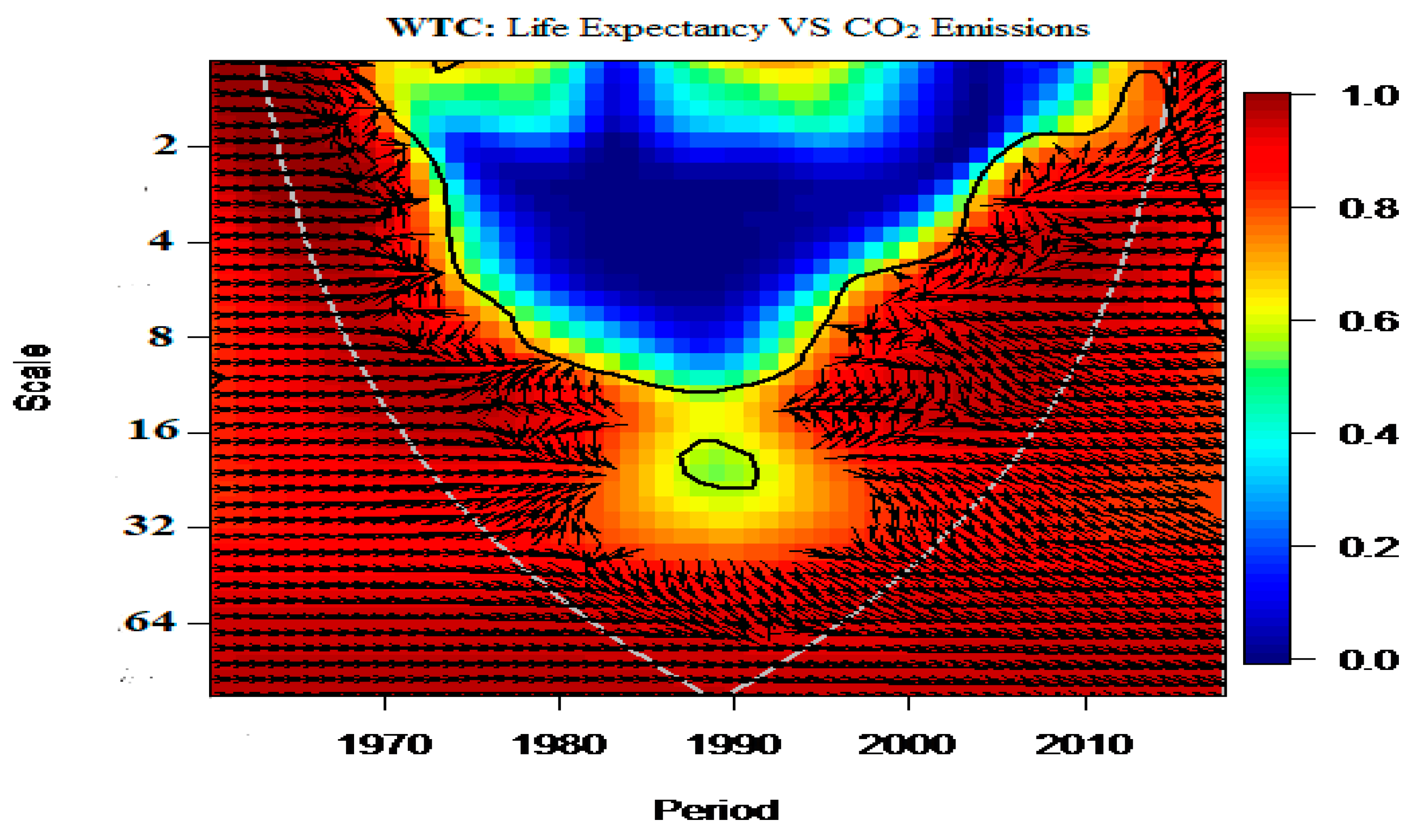
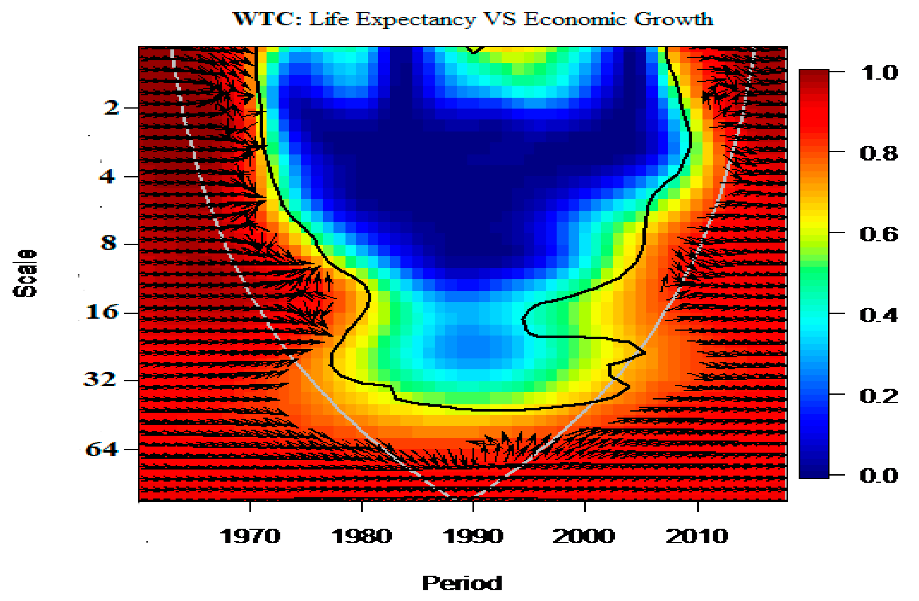
Interpretation is carried out inside the white cone, which is the cone of influence, in Figure 1 and Figure 2. In addition, the importance degree is shown by the thick black contour built on the simulations of Monte Carlo. According to Pal and Mitra [64] and Kirikkaleli and Adebayo [16], the time is shown on the horizontal axis, whereas the vertical axis displays the frequency. In Figure 1 and Figure 2, the higher the scale, the lower the frequency, and vice versa. The area of significant correlation is depicted by the warmer colors whilst lower dependence between the two time-series is illustrated by the cold colors (blue).
The arrows in Figure 1 and Figure 2 illustrate the lead/lag phase interconnection. A phase relationship is shown when the arrows point rightward (positive correlation between the two time-series) while the out of phase interconnection is shown when the arrows are facing leftward (negative correlation between the two time-series). Furthermore, rightward-up (leftward-down) arrows mean second variables lead the first variable while the rightward-down (leftward-up) arrows imply that the first variable leads the second variable. In Figure 1, at different scales (different frequencies), the arrows are facing rightward between 1964 and 2015. This implies that life expectancy and CO2 emissions are in phase (positive co-movement). Furthermore, the right-up arrows indicate that increased CO2 emissions led to decreased life expectancy in Turkey, which means CO2 emissions are a strong predictor of life expectancy. This finding is as expected since CO2 emissions deteriorate the quality of the environment, thereby causing harm to people’s health. This outcome is in contrast to the result of Balan [1], Agbanike et al. [2], Wang et al. [14], Wang et al. [31], and Zaidi and Saidi [38], while it is congruent with the studies of those that found a positive relationship between CO2 and life expectancy [3,4,9,40]. Figure 2 represents the wavelet coherence between life expectancy and economic growth from 1960 to 2018 in Turkey. Furthermore, between 1964 and 2015 at different scales (different frequencies) the arrows are rightward which indicates that life expectancy and economic growth are in phase (positive correlation). Additionally, the rightward-up arrows and rightward up arrows indicate a bidirectional causal interconnection between life expectancy and economic growth (see Figure 3). This indicates that life expectancy can predict economic growth and vice versa. This finding corresponds with the findings of Wang et al. [14], He and Li [15], Sirag et al. [22], and Biyase and Malesa [10].
The present study utilizes the Toda–Yamamoto and Fourier Toda–Yamamoto causality tests to investigate the time-domain causal interconnection between life expectancy and CO2 emissions and economic growth using a yearly dataset from 1960 to 2018. The Toda–Yamamoto test outcomes reveal no causal linkage between life expectancy and CO2 emissions, which indicates that the null hypothesis cannot be rejected at the 5% and 10% level of significance (see Table 4). This suggests that life expectancy does not lead to CO2 emissions. Furthermore, we find causality from CO2 emissions to life expectancy, implying that the hypothesis H1 is accepted at a 5% level of significance and suggesting that CO2 emissions can predict life expectancy and there is a causal relationship between carbon emissions and life expectancy in Turkey. In addition, we find evidence of a bidirectional causal interconnection between economic growth and life expectancy in Turkey. This illustrates that life expectancy and economic growth can predict each other. Therefore, H2 is accepted and there is a bidirectional causal relationship between life expectancy and economic growth. It is necessary to pinpoint that the Toda–Yamamoto test does not assume structural(s) amongst the variables. Hence, the study further employs the Fourier Toda–Yamamoto causality test, which considers the probable structural break(s) and the result presented in Table 4. The empirical findings of Fourier Toda–Yamamoto causality tests also affirm the outcome’s causal interconnection from CO2 emissions to life expectancy and the bidirectional causal link between economic growth and life expectancy, thus, the Fourier Toda–Yamamoto causality tests in the presence of structural break(s). It is worth noting that the findings of the Toda–Yamamoto and Fourier Toda–Yamamoto causality tests affirm the findings of the wavelet coherence technique.
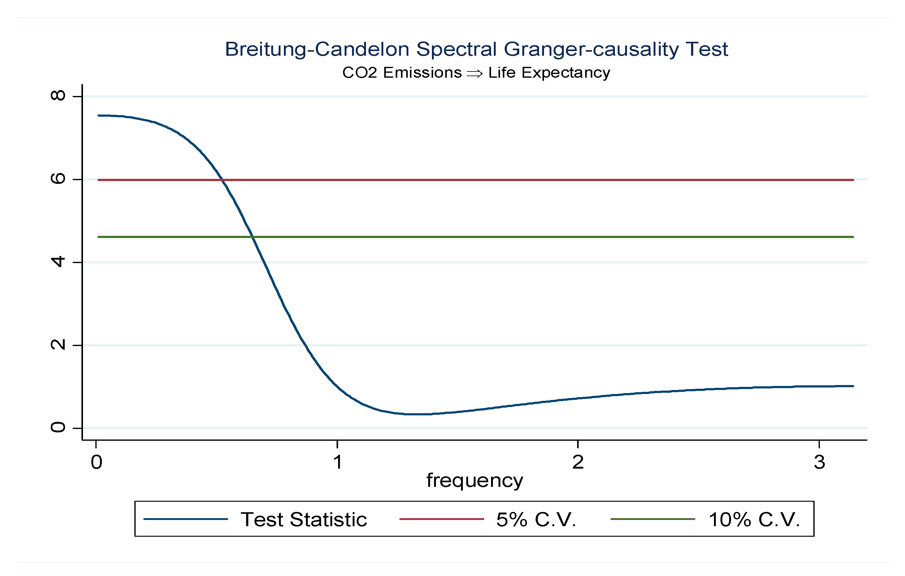
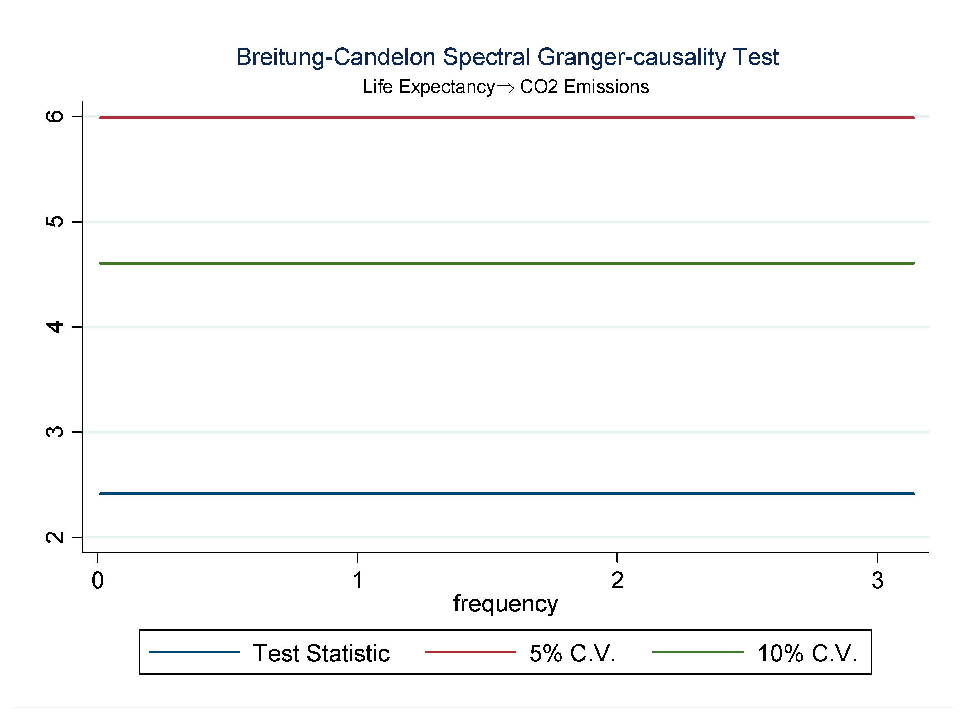
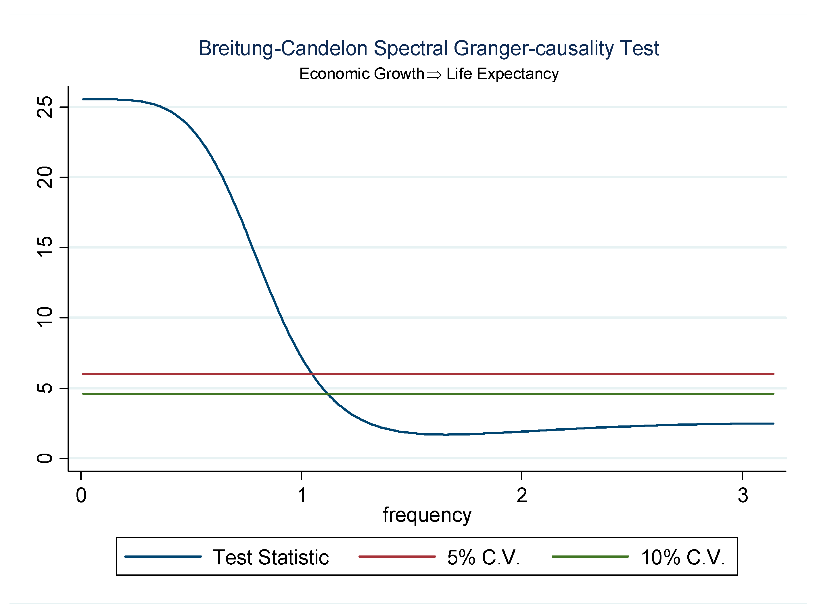
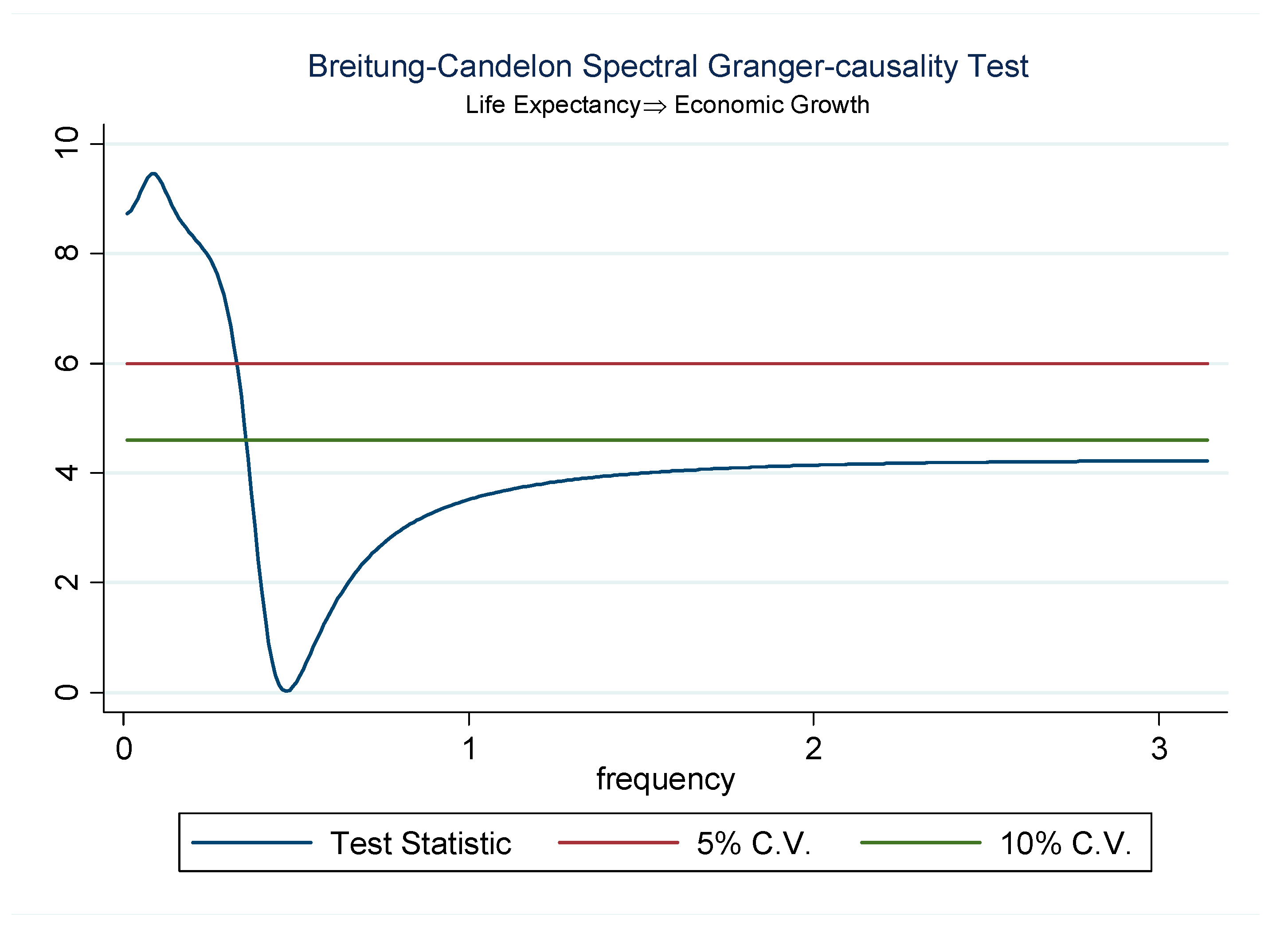
After exploring the causal interconnections between life expectancy, economic growth, and CO2 emissions by utilizing the time-domain causality tests, the study further employed the Breitung–Candelon frequency-domain spectral causality test to explore the causal impact of CO2 emissions and economic growth on life expectancy. When interpreting the frequency-domain spectral causality, the straight lines illustrate significance levels of 5 and 10% whereas the statistical tests at different frequencies between the intervals of (0, π) are represented by a curve. Figure 4 represents the causal linkage from CO2 emissions to life expectancy in Turkey. The finding reveals a causal interconnection between CO2 emissions and life expectancy in the short-, medium-, and long-run. The outcomes show that CO2 emissions can predict life expectancy in Turkey in the short-, medium-, and long-run, which implies that attention, should be given to CO2 emissions because they can hinder life expectancy. Figure 5 represents the causal interconnection from life expectancy to CO2 emissions in Turkey. The finding reveals no evidence of causal linkage from life expectancy to CO2 emissions in the short-, medium-, and long-run. As expected, this illustrates that life expectancy cannot predict CO2 emissions. The causal link from economic growth to life expectancy is illustrated in Figure 6. In the short run, there is no evidence of causal linkage from economic growth to life expectancy. This illustrates that the null hypothesis cannot be rejected at significance levels of 5 and 10%, respectively. However, in the medium- and long-run, there is evidence of causal linkage from economic growth to life expectancy. This illustrates that the null hypothesis is rejected at significance levels of 5 and 10%. This outcome shows that economic growth can predict life expectancy in Turkey in the medium- and long-run, which implies that consideration should be given to economic growth as it can improve the life expectancy of people in Turkey. Figure 7 reveals the causal interconnection from life expectancy to economic growth in Turkey. The finding reveals a causal association from life expectancy to economic growth in the short-, medium-, and long-run. This reveals that the null hypothesis is rejected at significance levels of 5 and 10%. This outcome shows that life expectancy can predict Turkey’s economic growth in the short-, medium-, and long-run, which infers that improving life expectancy can enhance economic growth in Turkey.

5. Conclusions and Inference

The increase in people’s life expectancy has resulted in the rapid aging and accumulation of productive factors all around the globe. Though the impact of life expectancy on economic growth is demonstrated in many studies, the positive or negative influence of economic growth on life expectancy is still an open problem. In addition, some studies found a significant relationship between CO2 and life expectancy. Meanwhile, it is possible to get a causal relationship among economic growth, carbon emissions, and life expectancy because economic growth triggers carbon emissions, and result in environmental degradation with its consequence on the health outcomes like life expectancy and overall sustainable development. The relationships have not been previously investigated, especially in the case of Turkey. Therefore, in this paper, we investigate the sustainable causal relationship among the three variables. To do so, in this paper, we test the following hypotheses: (i) a bidirectional relationship between life expectancy and economic growth and (ii) a causal relationship between carbon emissions and life expectancy. To test whether the hypotheses hold, we used the long time-series data from 1960 to 2018 and employed the overlapping generational model that provides a theoretical background for the study. We employ both ADF and PP unit root tests to examine orders of integration for the variables, use Zivot–Andrews and Lee–Strazicich unit root tests to test whether there is any structural break in the series, use the Bayer–Hanck cointegration test to conduct a robust cointegration analysis that reveals the existence of long-run cointegration among the variables, and employ both time and frequency-domain causality tests by using wavelet coherence and Fourier Toda–Yamamoto techniques to investigate the cause and direction of the relationship that exist between economic growth and life expectancy on the one hand, and the CO2 emissions and life expectancy on the other hand, in addition to examining the effects of economic growth and CO2 emissions on life expectancy at different frequencies in Turkey.
Different from existing studies that focus on the directional causal relationship between economic growth and life expectancy on the one hand, and CO2 and life expectancy on the other hand, we examine the time and frequency domain causality between the variables using the wavelet coherence techniques. The methods provide evidence that there is a positive co-movement between life expectancy and CO2 emissions, showing that CO2 is a strong predictor of life expectancy, and there are positive correlations between life expectancy and economic growth at different scales. In addition, the Fourier Toda–Yamamoto causality test was used to explore the time-domain causality between economic growth, CO2, and life expectancy. The finding reveals that CO2 emissions influence life expectancy, establishing a bidirectional relationship between life expectancy and economic growth. Another novel finding of our study is the use of the Breitung–Candelon frequency-domain spectral causality test to examine the causality among the variables at different stages. The results show that CO2 has short-, medium-, and long-run causal relationships with LE and GDP has medium and long-run causal relationships with life expectancy, while life expectancy has short-, medium-, and long-run causal relationships with economic growth. Generally, our study provides new empirical evidence justifying the causal relationships among GDP, CO2, and LE in Turkey.
Our findings infer that the policymakers in Turkey should revise their strategies and policies that will ensure the sustainability of the relationship between energy consumption and environmental degradation, so as to ensure the protection of human health and their longevity that will contribute to the overall sustainable development. In addition, the budgetary allocation to the health sector should be improved so that the health-related challenges could arise from environmental hazards that cause health-related problems and affect longevity would be tackled. More importantly, the allocation to science and technology should be increased so that the technological capabilities of the country can be enhanced, geared towards moving away from the consumption of non-renewable energy that is triggering CO2 emissions which could affect the achievement of environmental sustainability in the country. In Turkey, policymakers should strengthen well-functioning environmental agencies that are charged with the responsibility of enforcing environmental regulations with the view of ensuring environmental quality. Moreover, the mandatory significant reductions in emissions in Turkey should be implemented to ensure the reduction of carbon emissions in the country, which no doubt will contribute significantly to the environmental sustainability of the country.
This study highlights both the prospective and empirical effects of carbon emissions and economic growth on life expectancy in Turkey. The evidence is apparent to support policies and programs that will be developed and implemented to address high levels of carbon emissions in Turkey and reduce pollution-induced health issues that could affect people’s longevity and environmental sustainability. Moreover, the new econometric techniques employed in the study provide more empirical insights for academics to achieve unbiased estimations.
The limitations of our study lie in the use of CO2 emissions as a proxy for environmental pollution; thus, future studies could utilize other forms of pollutants like NOx, NO2, NO, PM2.5, etc. to agree or disagree with the findings from this study. In addition, this study was basically on Turkey with a peculiar nature which has the possibility of limiting the generalization of the study; therefore, future studies can replicate the model in another developing country or a comparative study of two countries. Nevertheless, this study makes significant contributions that are useful for academics, practitioners, and policymakers in addressing the issue of the relationship between environmental quality, economic growth, and life expectancy.

Author Contributions

Conceptualization, H.R. and J.A.O.; methodology, T.S.A. and J.A.O.; J.A.O. and T.S.A.; formal analysis, J.A.O. and T.S.A.; investigation, H.R.; resources, J.A.O. and T.S.A.; data curation, J.A.O.; writing—original draft preparation, H.R., J.A.O. and T.S.A.; writing—review and editing, W.-K.W.; supervision, H.R. and W.-K.W.; project administration, H.R.; funding acquisition, W.-K.W. All authors have read and agreed to the published version of the manuscript.

Funding

The APC was funded by W.-K.W.

Institutional Review Board Statement

The study was conducted according to the research guidelines approved by the Ethics Committees of Authors Institutions.

Informed Consent Statement

Not applicable.

Data Availability Statement

Not applicable.

Conflicts of Interest

The authors declare no conflict of interest.

References

  1. Balan, F. Environmental quality and its human health effects: A causal analysis for the EU-25. Int. J. Appl. Econ. 2016, 13, 57–71. [Google Scholar]
  2. Agbanike, T.F.; Nwani, C.; Uwazie, U.; Uma, K.E.; Anochiwa, L.; Igberi, C.; Ogbonnaya, I.O. Oil, Environmental Pollution and Life Expectancy In Nigeria. Appl. Ecol. Environ. Res. 2019, 17, 11143–11162. [Google Scholar] [CrossRef]
  3. Balakrishnan, K.; Dey, S.; Gupta, T.; Dhaliwal, R.S.; Brauer, M.; Cohen, A.J.; Sabde, Y. The impact of air pollution on deaths, disease burden, and life expectancy across the states of India: The Global Burden of Disease Study 2017. Lancet Planet. Health 2019, 3, e26–e39. [Google Scholar] [CrossRef] [Green Version]
  4. Schwartz, J.D.; Wang, Y.; Kloog, I.; Yitshak-Sade, M.A.; Dominici, F.; Zanobetti, A. Estimating the effects of PM2.5 on life expectancy using causal modeling methods. Environ. Health Perspect. 2018, 126, 127002. [Google Scholar] [CrossRef] [PubMed] [Green Version]
  5. Adebayo, T.S.; Odugbesan, J.A. Modeling CO2 emissions in South Africa: Empirical evidence from ARDL based bounds and wavelet coherence techniques. Environ. Sci. Pollut. Res. 2020, 1–13. [Google Scholar] [CrossRef]
  6. Odugbesan, J.A.; Adebayo, T.S. The symmetrical and asymmetrical effects of foreign direct investment and financial development on carbon emission: Evidence from Nigeria. SN Appl. Sci. 2020, 2, 1–15. [Google Scholar] [CrossRef]
  7. Rjoub, H.; Odugbesan, J.A.; Adebayo, T.S.; Wong, W.K. Sustainability of the Moderating Role of Financial Development in the Determinants of Environmental Degradation: Evidence from Turkey. Sustainability 2021, 13, 1844. [Google Scholar] [CrossRef]
  8. Odusanya, I.A.; Adegboyega, S.B.; Kuku, M.A. Environmental Quality and Health Care Spending In Nigeria. Fountain J. Manag. Soc. Sci. 2014, 3, 57–67. [Google Scholar]
  9. Mariani, F.; Pérez-Barahona, A.; Raffin, N. Life expectancy and the environment. J. Econom. Dyn. Control 2010, 34, 798–815. [Google Scholar] [CrossRef]
  10. Biyase, M.; Malesa, M. Life Expectancy and Economic Growth: Evidence from the Southern African Development Community. Econ. Internazionale/Int. Econ. 2019, 72, 351–366. Available online: http://www.iei1946.it/en/rivista-articolo.php?id=197 (accessed on 10 December 2020).
  11. Alam, M.S.; Shahbaz, M.; Paramati, S.R. The role of financial development and economic misery on life expectancy: Evidence from post reforms in India. Soc. Indic. Res. 2016, 128, 481–497. [Google Scholar] [CrossRef]
  12. Shahbaz, M.; Loganathan, N.; Mujahid, N.; Ali, A.; Nawaz, A. Determinants of life expectancy and its prospects under the role of economic misery: A case of Pakistan. Soc. Indic. Res. 2016, 126, 1299–1316. [Google Scholar] [CrossRef] [Green Version]
  13. Wu, C. Human capital, life expectancy, and the environment. J. Int. Trade Econ. Dev. 2017, 26, 885–906. [Google Scholar] [CrossRef]
  14. Wang, Z.; Asghar, M.M.; Zaidi, S.A.H.; Nawaz, K.; Wang, B.; Zhao, W.; Xu, F. The dynamic relationship between economic growth and life expectancy: Contradictory role of energy consumption and financial development in Pakistan. Struct. Chang. Econ. Dyn. 2020, 53, 257–266. [Google Scholar] [CrossRef]
  15. He, L.; Li, N. The linkages between life expectancy and economic growth: Some new evidence. Empir. Econ. 2020, 58, 2381–2402. [Google Scholar] [CrossRef]
  16. Kirikkaleli, D.; Adebayo, T.S. Do public-private partnerships in energy and renewable energy consumption matter for consumption-based carbon dioxide emissions in India? Environ. Sci. Pollut. Res. 2021, 1–14. [Google Scholar] [CrossRef]
  17. World Bank. World Development Indicators. Available online: http://data.worldbank.org/ (accessed on 30 September 2020).
  18. Bilgen, S.; Keleş, S.; Kaygusuz, A.; Sarı, A.; Kaygusuz, K. Global warming and renewable energy sources for sustainable development: A case study in Turkey. Renew. Sustain. Energy Rev. 2008, 12, 372–396. [Google Scholar] [CrossRef]
  19. TUIK. Main Statistics. Available online: http://www.turkstat.gov.tr (accessed on 30 May 2020).
  20. Gövdeli, T. Life Expectancy, Direct Foreign Investments, Trade Openness and Economic Growth in E7 Countries: Heterogeneous Panel Analysis. Third Sect. Soc. Econ. Rev. 2019, 54, 731–743. [Google Scholar] [CrossRef]
  21. Shahbaz, M.; Shafiullah, M.; Mahalik, M.K. The dynamics of financial development, globalisation, economic growth and life expectancy in sub-Saharan Africa. Aust. Econ. Pap. 2019, 58, 444–479. [Google Scholar] [CrossRef]
  22. Sirag, A.; Norashidah, M.N.; Law, S.H. Does higher longevity harm economic growth? Panoeconomicus 2020, 67, 51–68. [Google Scholar] [CrossRef] [Green Version]
  23. Yakita, A. Life expectancy, money, and growth. J. Political Econ. 2006, 19, 579–592. [Google Scholar] [CrossRef]
  24. Kalemli-Ozcan, S.; Ryder, H.E.; Weil, D.N. Mortality decline, human capital investment, and economic growth. J. Dev. Econ. 2000, 62, 1–23. [Google Scholar] [CrossRef]
  25. Acemoglu, D.; Johnson, S. Disease and development: The effect of life expectancy on economic growth. J. Political Econ. 2007, 115, 925–985. [Google Scholar] [CrossRef] [Green Version]
  26. Leung, M.C.; Wang, Y. Endogenous health care, life expectancy and economic growth. Pac. Econ. Rev. 2010, 15, 11–31. [Google Scholar] [CrossRef]
  27. Boucekkine, R.; La Croix, D.D.; Licandro, O. Vintage human capital, demographic trends, and endogenous growth. J. Econom. Theory 2002, 104, 340–375. [Google Scholar] [CrossRef] [Green Version]
  28. Echevarría, C.A. Life expectancy, schooling time, retirement, and growth. Econ. Inq. 2004, 42, 602–617. [Google Scholar] [CrossRef]
  29. Kunze, L. Life expectancy and economic growth. J. Macroecon. 2014, 39, 54–65. [Google Scholar] [CrossRef]
  30. Martins, F.; Felgueiras, C.; Smitkova, M.; Caetano, N. Analysis of fossil fuel energy consumption and environmental impacts in European countries. Energies 2019, 12, 964. [Google Scholar] [CrossRef] [Green Version]
  31. Wang, Z.; Asghar, M.M.; Zaidi, S.A.H.; Wang, B. Dynamic linkages among CO2 emissions, health expenditures, and economic growth: Empirical evidence from Pakistan. Environ. Sci. Pollut. Res. 2019, 26, 15285–15299. [Google Scholar] [CrossRef] [PubMed]
  32. Sarkodie, S.A.; Strezov, V.; Jiang, Y.; Evans, T. Proximate determinants of particulate matter (PM2.5) emission, mortality and life expectancy in Europe, Central Asia, Australia, Canada and the US. Sci. Total Environ. 2019, 683, 489–497. [Google Scholar] [CrossRef]
  33. Adebayo, T.S.; Kalmaz, D.B. Determinants of CO2 emissions: Empirical evidence from Egypt. Environ. Ecol. Stat. 2021, 1–24. [Google Scholar] [CrossRef]
  34. Zaidi, S.A.H.; Danish; Hou, F.; Mirza, F.M. The role of renewable and non-renewable energy consumption in CO2 emissions: A disaggregate analysis of Pakistan. Environ. Sci. Pollut. Res. 2018, 25, 31616–31629. [Google Scholar] [CrossRef]
  35. Bekhet, H.A.; Matar, A.; Yasmin, T. CO2 emissions, energy consumption, economic growth, and financial development in GCC countries: Dynamic simultaneous equation models. Renew. Sustain. Energy Rev. 2017, 70, 117–132. [Google Scholar] [CrossRef]
  36. Wang, B.; Wang, Z. Imported technology and CO2 emission in China: Collecting evidence through bound testing and VECM approach. Renew. Sustain. Energy Rev. 2018, 82, 4204–4214. [Google Scholar] [CrossRef]
  37. Zakaria, M.; Bibi, S. Financial development and environment in South Asia: The role of institutional quality. Environ. Sci. Pollut. Res. 2019, 26, 7926–7937. [Google Scholar] [CrossRef]
  38. Zaidi, S.; Saidi, K. Environmental pollution, health expenditure and economic growth in the Sub-Saharan Africa countries: Panel ARDL approach. Sustain. Cities Soc. 2018, 41, 833–840. [Google Scholar] [CrossRef]
  39. Al-Mulali, U.; Ozturk, I. The effect of energy consumption, urbanization, trade openness, industrial output, and the political stability on the environmental degradation in the MENA (Middle East and North African) region. Energy 2015, 84, 382–389. [Google Scholar] [CrossRef]
  40. Issaoui, F.; Toumi, H.; Touili, W. The effects of carbon dioxide emissions on economic growth, urbanization, and welfare. J. Energy Dev. 2015, 41, 223–252. Available online: https://www.jstor.org/stable/10.2307/90005938 (accessed on 10 December 2020).
  41. Clootens, N. Public debt, life expectancy, and the environment. Environ. Modeling Assess. 2017, 22, 267–278. [Google Scholar] [CrossRef]
  42. Ono, T.; Maeda, Y. Sustainable development in an aging economy. Environ. Dev. Econ. 2002, 7, 9–22. [Google Scholar] [CrossRef] [Green Version]
  43. Pecchenino, R.; Pollard, P. The effects of annuities, bequests and aging in an overlapping generations model of endogenous growth. Econ. J. 1997, 107, 26–46. [Google Scholar] [CrossRef] [Green Version]
  44. John, A.; Pecchenino, R. An overlapping generations model of growth and the environment. Econ. J. 1994, 104, 1393. [Google Scholar] [CrossRef]
  45. Elo, I.T.; Preston, S.H. Effects of early-life conditions on adult mortality: A review. Popul. Index 1992, 58, 186–212. Available online: https://www.jstor.org/stable/3644718 (accessed on 10 December 2020). [CrossRef] [PubMed]
  46. Pope, C.A.; Burnett, R.T.; Thurston, G.D.; Thun, M.J.; Calle, E.E.; Krewski, D.; Godleski, J.J. Cardiovascular mortality and longterm exposure to particulate air pollution: Epidemiological evidence of general pathophysiological pathways of disease. Circulation 2004, 109, 71–77. [Google Scholar] [CrossRef] [PubMed] [Green Version]
  47. Evans, M.F.; Smith, V.K. Do new health conditions support mortality-air pollution effects? J. Environ. Econ. Manag. 2005, 50, 496–518. [Google Scholar] [CrossRef]
  48. Zivot, E.; Andrews, D.W.K. Further evidence on the great crash, the oil-price shock, and the unit-root hypothesis. J. Bus. Econ. Stat. 2002, 20, 25–44. [Google Scholar] [CrossRef]
  49. Lee, J.; Strazicich, M.C. Minimum Lagrange multiplier unit root test with two structural breaks. Rev. Econ. Stat. 2003, 85, 1082–1089. [Google Scholar] [CrossRef]
  50. Phillips, P.C.; Perron, P. Testing for a unit root in time series regression. Biometrika 1988, 75, 335–346. [Google Scholar] [CrossRef]
  51. Vougas, D.V. Reconsidering LM unit root testing. J. Appl. Stat. 2003, 30, 727–741. [Google Scholar] [CrossRef]
  52. Bayer, C.; Hanck, C. Combining non-cointegration tests. J. Time Ser. Anal. 2013, 34, 83–95. [Google Scholar] [CrossRef]
  53. Engle, R.F.; Granger, C.W. Co-integration and error correction: Representation, estimation, and testing. Econ. J. Econom. Soc. 1987, 251–276. Available online: https://www.jstor.org/stable/1913236 (accessed on 10 December 2020). [CrossRef]
  54. Boswijk, H.P. Testing for an unstable root in conditional and structural error correction models. J. Econom. 1994, 63, 37–60. [Google Scholar] [CrossRef]
  55. Johansen, S. Estimation of cointegration vectors in Gaussian vector autoregressive models. Econom. J. Econom. Soc. 1991, 59, 1551–1580. Available online: https://www.jstor.org/stable/2938278 (accessed on 10 December 2020).
  56. Banerjee, A.; Dolado, J.; Mestre, R. Error-correction mechanism tests for cointegration in a single-equation framework. J. Time Ser. Anal. 1998, 19, 267–283. [Google Scholar] [CrossRef] [Green Version]
  57. Bekun, F.V.; Emir, F.; Sarkodie, S.A. Another look at the relationship between energy consumption, carbon dioxide emissions, and economic growth in South Africa. Sci. Total Environ. 2019, 655, 759–765. [Google Scholar] [CrossRef] [PubMed]
  58. Goupilaud, P.; Grossmann, A.; Morlet, J. Cycle-octave and related transforms in seismic signal analysis. Geoexploration 1984, 23, 85–102. [Google Scholar] [CrossRef]
  59. Torrence, C.; Compo, G.P. A practical guide to wavelet analysis. Bull. Am. Meteorol. Soc. 1998, 79, 61–78. [Google Scholar] [CrossRef] [Green Version]
  60. Toda, H.Y.; Yamamoto, T. Statistical inference in vector autoregressions with possibly integrated processes. J. Econom. 1995, 66, 225–250. [Google Scholar] [CrossRef]
  61. Breitung, J.; Candelon, B. Testing for short-and long-run causality: A frequency-domain approach. J. Econom. 2006, 132, 363–378. [Google Scholar] [CrossRef]
  62. Adebayo, T.S. Revisiting the EKC hypothesis in an emerging market: An application of ARDL-based bounds and wavelet coherence approaches. SN Appl. Sci. 2020, 2, 1–15. [Google Scholar] [CrossRef]
  63. Buonanno, P.; Carraro, C.; Galeotti, M. Endogenous induced technical change and the costs of Kyoto. Resour. Energy Econ. 2003, 25, 11–34. [Google Scholar] [CrossRef] [Green Version]
  64. Pal, D.; Mitra, S.K. Time-frequency contained co-movement of crude oil and world food prices: A wavelet-based analysis. Energy Econ. 2017, 62, 230–239. [Google Scholar] [CrossRef]
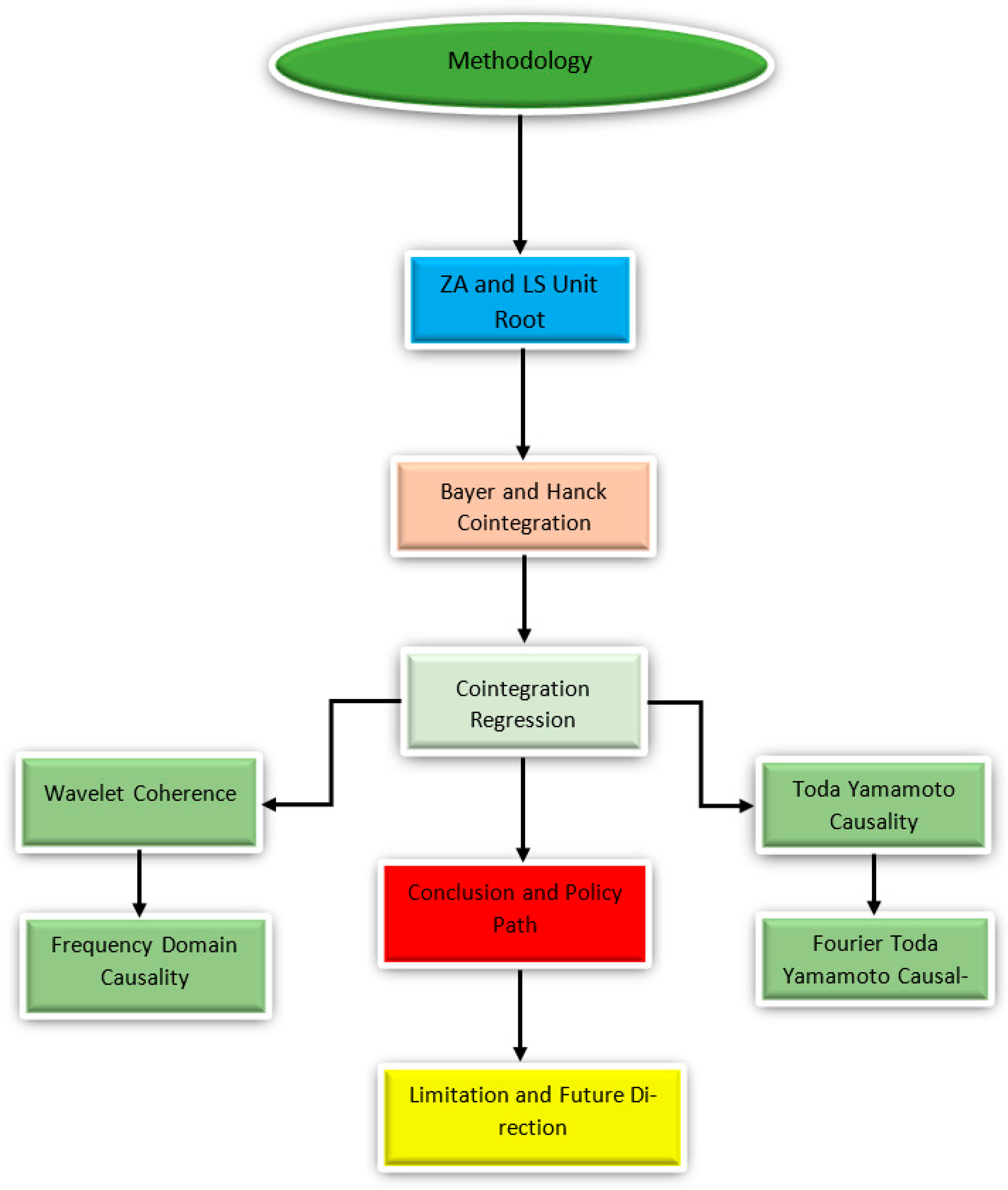
Figure 1. Analysis Flow Chart.
Sustainability 13 02924 g001
Figure 2. WTC between life expectancy and CO2 emissions. Source: Authors Compilation with R-Software.
Sustainability 13 02924 g002
Figure 3. WTC between life expectancy and economic growth. Source: Authors Compilation with R-Software.
Sustainability 13 02924 g003
Figure 4. Spectral causality from CO2 emissions to life expectancy. Source: Authors Compilation with Stata-Software.
Sustainability 13 02924 g004
Figure 5. Spectral causality from life expectancy to CO2 emissions. Source: Authors Compilation with Stata-Software.
Sustainability 13 02924 g005
Figure 6. Spectral causality from economic growth to life expectancy. Source: Authors Compilation with Stata-Software.
Sustainability 13 02924 g006
Figure 7. Spectral causality from life expectancy to economic growth. Source: Authors Compilation with Stata-Software.
Sustainability 13 02924 g007
Table 1. Descriptive Statistics.
VariableLife ExpectancyCO2 EmissionsEconomic Growth
CodeLFCO2GDP
Time1960–2018
Mean63.117902.5860487229.986
Median63.763002.6289896404.016
Maximum77.437005.09000015068.98
Minimum45.369000.6122713134.777
Std. Dev.9.6422001.2493663226.139
Skewness−0.1939390.2172690.855215
Kurtosis1.8100462.0165452.819231
Jarque–Bera3.8508322.8418497.272362
Probability0.1458150.2414910.026353
Observations595959
Table 2. Unit root Tests.
Lee–Strachwich Unit-RootZivot–Andrews Unit-Root
t-StatisticSB1SB2t-StatisticSB1
At levels
LEK&T−9.711 *19792005−1.3592003
CO2−5.755 **19942000−5.222 **2001
GDP−5.48619952008−4.2792001
At first difference
LEK&T−13.01 *19811997−6.889 *1995
CO2−8.113 *19751999−6.885 *1978
GDP−7.328 *19881992−7.847 *2003
Note: * and ** illustrates a 1 and 5% level of significance. SB1 and SB2 stand for one and two structural breaks, respectively.
Table 3. Bayer–Hanch cointegration test.
Model SpecificationsFisher StatisticsFisher StatisticsCointegration Decision
EG-JOHEG-JOH-BAN-BOS
LE = f(CO2, GDP)14.291 **25.813 ***Yes
Critical valueCritical value
Significance level at 5%10.57620.143
Note: ** and *** illustrates 5% and 10% level of significance, respectively.
Table 4. Toda–Yamamoto and Fourier Toda–Yamamoto Tests.
Toda–Yamamoto Causality TestFourier Toda–Yamamoto Test
Direction of CausalityMwald-StatWald-StatDecision
LE→CO23.9128.511Do not reject Ho
CO2→LE8.612 ***13.095 ***Reject Ho
LE→GDP7.319 *13.126 ***Reject Ho
GDP→LE8.208 *16.225 **Reject Ho
Note: *, **, and *** denotes 1, 5, and 10% level of significance, respectively.
Publisher’s Note: MDPI stays neutral with regard to jurisdictional claims in published maps and institutional affiliations.