Assessing the Impact of Greenhouse Gas Emissions on Economic Profitability of Arable, Forestry, and Silvoarable Systems

Abstract

This study assesses the greenhouse gas (GHG) emissions and sequestration of a silvoarable system with poplar trees and a crop rotation of wheat, barley, and oilseed rape and compares this with a rotation of the same arable crops and a poplar plantation. The Farm-SAFE model, a financial model of arable, forestry, and silvoarable systems, was modified to account for life-cycle greenhouse gas emissions. Greenhouse gas emissions from tree and crop management were determined from life-cycle inventories and carbon storage benefits from the Yield-SAFE model, which predicts crop and tree yields in arable, forestry, and silvoarable systems. An experimental site in Silsoe in southern England served as a case study. The results showed that the arable system was the most financially profitable system, followed by the silvoarable and then the forestry systems, with equivalent annual values of EUR 560, 450 and 140 ha⁻¹, respectively. When the positive and negative externalities of GHG sequestration and emissions were converted into carbon equivalents and given an economic value, the profitability of the arable systems was altered relative to the forestry and silvoarable systems, although in the analysis, the exact impact depended on the value given to GHG emissions. Market values for carbon resulted in the arable system remaining the most profitable system, albeit at a reduced level. Time series values for carbon proposed by the UK government resulted in forestry being the most profitable system. Hence, the relative benefit of the three systems was highly sensitive to the value that carbon was given in the analysis. This in turn is dependent on the perspective that is given to the analysis.

1. Introduction

Around one-third of human-induced greenhouse gas (GHG) emissions are assigned to global food production, with agricultural production being the largest source [1,2]. Food production is also particularly vulnerable to the effects of climate change [3]. Elevated anthropogenic GHG emissions have led to the introduction of international treaties and national targets (e.g., the UK 2008 Climate Change Act and the 2016 Paris Agreement) to reduce GHG emissions and hence mitigate potential impacts of climate change.

For several decades, the complexity of agriculture and forestry has been reduced through intensification, mechanisation as well as consolidation of agricultural land in order to simplify management and increase efficiency [4,5]. This has led to modern agriculture being highly reliant on external inputs [6,7,8] which alter and affect natural habitats, landscapes, plants and animals [9]. Such management of agricultural land is associated with adverse environmental impacts such as diffuse pollution (nutrient leaching and runoff of agrochemicals), soil degradation (e.g., erosion, compaction and loss of soil organic matter), loss of biodiversity (including pollinators), increased demand for non-renewable natural resources (e.g., fossil energy resources, phosphorus), pollution of water, soil and GHG (“carbon”) emissions [7,10]. Such externalities are rarely accounted for in cost-benefit analyses of agricultural enterprises, since they are non-market by nature and economic data for them is therefore difficult to obtain.

Without major change, these adverse effects are expected to become more serious as population growth, economic development, and changes in dietary behaviour increase pressure on land and resources [11,12]. The agriculture sector faces the prospect of feeding a projected population of 9 to 10 billion people by 2050, hence needing increased commodity production by about 60–70% [13,14]. Increased land use change would be required for the production of some commodities, but GHG emissions need to be cut at the same time. It has been identified that climate change requires “the rethinking and refashioning of agriculture” [3] in order to increase resilience and robustness of the whole food system. Hence, the main challenge is to make agricultural and food systems more productive while making them more sustainable [10].

Introducing woody species on agricultural land reduces GHG emissions while increasing carbon sequestration [15]. Agricultural production systems that include trees are defined as agroforestry systems, which can be classified as silvoarable (crops and trees), silvopastoral (pasture/animals and trees) or agrosilvopastoral (crops, pasture/animals and trees) systems [16].

Various studies have found an expanded range of ecosystem services provided by agroforestry [5,13,17,18], including especially the potential for carbon sequestration which contributes to climate regulation [19,20]. Other regulating services have also been identified, such as the reduction of nitrogen leaching from use of fertiliser in agricultural production systems [21]. There is a large potential for the transition of arable systems to silvoarable systems in the UK, as approximately 28% of 17.5 million ha agricultural land are used for crop production [22]. Factors that hinder the uptake of agroforestry and what the financial and economic implications are, are not well understood.

Modelling is required to analyse the long rotation cycles that are typical of agroforestry. Graves et al. [23] developed the Farm-SAFE model to compare the profitability of monocultures and silvoarable agroforestry systems. This was limited to financial costs and benefits and did not address externalities, such as GHG emissions. Various studies have been conducted during recent years to quantify the environmental burdens of agricultural commodities, using life cycle assessment in different production systems [6,7,24,25]. While some of these studies have taken a holistic perspective [10] by quantifying, and sometimes integrating, various impact categories (e.g., acidification, eutrophication, resource depletion, and climate change) many focus only on GHG emissions, or the carbon footprint, as defined by the British Standards Institution [26]. Most of them focus in their analysis on per unit output of arable crops, although some address the whole rotation, such as Goglio et al. [27]. The same is true for life cycle assessment studies in the forestry industry [28,29,30,31,32,33].

The overall aim of this study was to quantify the GHG emissions and above-ground C sequestration of a silvoarable agroforestry system relative to an arable and forestry counterfactual over an entire tree rotation and to estimate and compare the economic performance of the three land uses.

2. Method

This work further developed the existing financial model, Farm-SAFE, an Excel-based spreadsheet model developed by Graves et al. [23] by consolidating market data on costs and benefits with life cycle inventory and valuation data, in order to consider the monetised environmental burdens and benefits within an economic appraisal. The emphasis of the life cycle inventory was placed on GHG emissions of on-field machinery operations and fertiliser and pesticide use. The ‘extended FarmSAFE’ model was than applied to a case study in the UK to derive an integrated market and non-market valuation of an arable, silvoarable agroforestry, and forestry system.

The method used in this study involved five different steps: (i) estimation of financial costs and benefits of an arable, forestry and agroforestry system, (ii) identification and quantification of the GHG emissions arising from machinery operations and use of agrochemicals, (iii) calculation of GHG benefits from carbon sequestration, (iv) conversion of the externalities arising from machinery operations and use of agrochemicals and carbon sequestration into monetary terms, and (v) comparison of financial and economic profitability of the three production systems.

2.1. Case Study Description

An experimental plot of a silvoarable agroforestry system in Silsoe in South East England (52.00852° N 0.42378° W) (Figure 1) was chosen as a case study site [34]. Average annual precipitation in the site was around 630 mm and irrigation was not needed. The soil type at the site consisted in 50% clay and 50% sand [34].

A 30-year time horizon was assumed for the analysis as this is a typical rotation length for poplar in the UK. No thinning of trees was assumed in both the forestry and the agroforestry system. The output equivalency of the different systems was established through a comparison on a per hectare basis [27]. The evaluated production systems were:

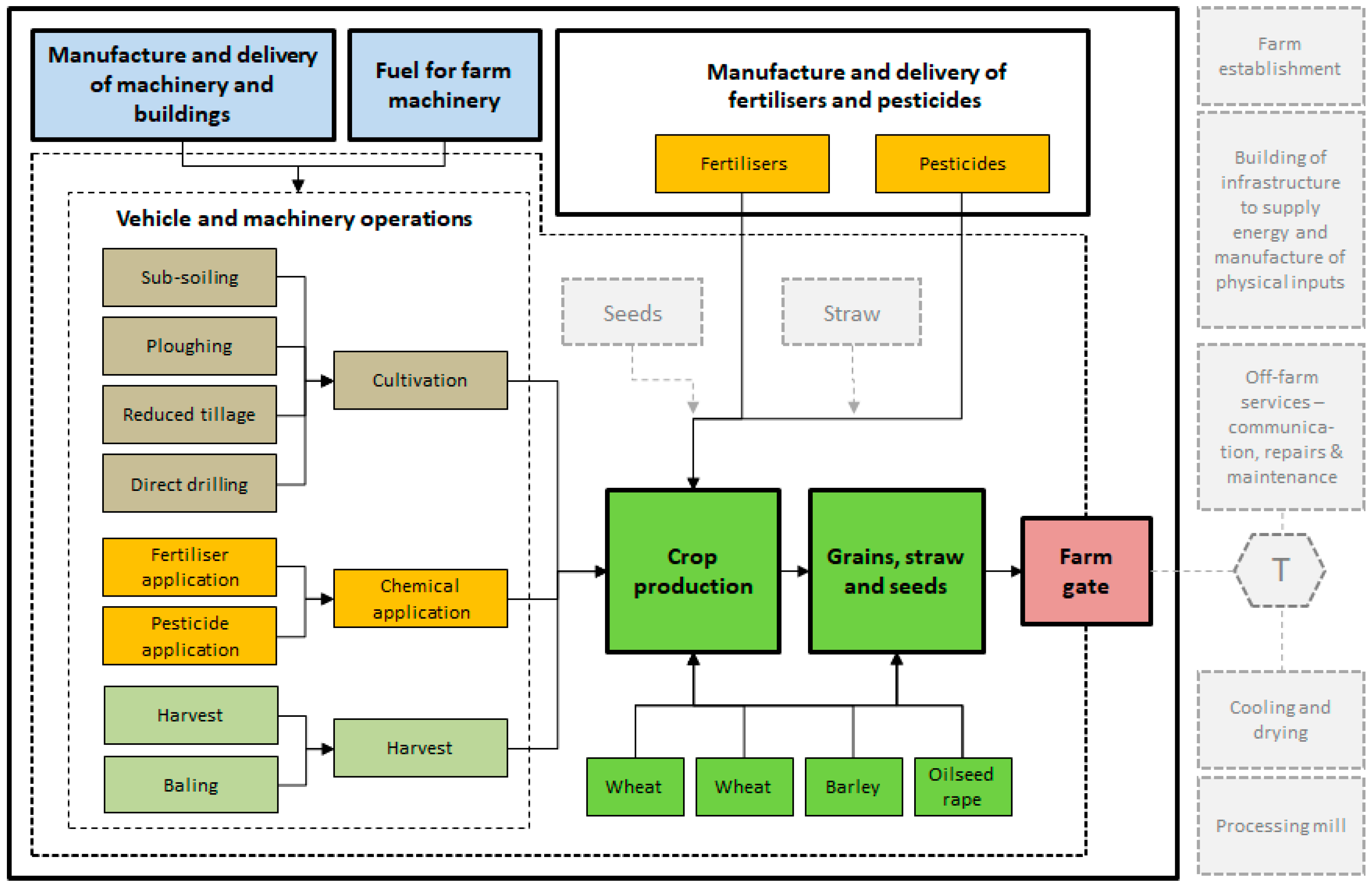
• Arable: A four-year rotation of autumn sown winter wheat (feed), winter wheat (feed), winter barley (feed), and winter oilseed rape over a time horizon of 30 years.
• Forestry: A poplar (Populus spp.) hybrid (Beaupré) over a rotation of 30 years.
• Agroforestry: Silvoarable system with the poplar (Populus spp.) hybrid (Beaupré) over a rotation of 30 years and a four-year crop rotation identical to that of the arable system.

2.2. Input Data

2.2.1. Biophysical Data

The biophysical data for biomass accumulation of crops and woody species were simulated with the Yield-SAFE model [35]. Yield-SAFE accounted for seasonal variability and considered abiotic factors (e.g., soil types and daily climatic conditions such as temperature, precipitation, radiation and relative humidity). Calibration of the Yield-SAFE model was based on the Silsoe case study [34].

2.2.2. Financial Data

The Farm-SAFE model was utilized to calculate financial performance. UK-specific crop management input data were obtained from typical farm management practices [36]. A constant grain price was assumed for the full crop rotation cycle, based on average values expected for 2016. The grant scheme was based on the Common Agricultural Policy (CAP) Basic Payment Scheme (BPS) for lowlands in England [36].

Data on the establishment, management and logging of the tree component were obtained from various sources. The silvicultural practices were based on Savill [37] and the incurred costs and labour inputs were derived from the experimental plot for the Silsoe case study. The woodland creation grant was assumed for the forestry and agroforestry systems, which provided EUR 2361 ha⁻¹ for wide-spaced broadleaved systems [36]. In this, 80% of the planting grants were paid upon completion of tree establishment in the first year. The payment of the remaining 20% was linked to the woodlands still being properly maintained in Year 5. All prices and costs were converted from British pounds into euros assuming a typical exchange rate of 1.3 euros per British pound between 2015 and 2016.

2.2.3. Life-Cycle Data

The life-cycle inventory (LCI) data were compiled from various sources. The LCI for this study came from the LCA model developed by Williams et al. [25] and provided LCI data on resource inputs, operating rates of machinery and emission inventory for the arable crop rotation. Tree component data were obtained from González-García et al. [28], Morison et al. [38] and Williams et al. [25] and adjusted to the respective tree management of the forestry and agroforestry systems.

For crops, all field activities were assumed to be optimised, and hence tractors with different engine powers were matched to each field operation. The system boundaries (Figure 2 and Figure 3) included GHG emissions from diesel used for field operations, the manufacture of diesel, tractors, related field implements and agrochemical manufacture and use. Straw was assumed to be collected and sold. In contrast to forestry management over large areas of land, which relies heavily on forest machinery [39], it was assumed that much of the work (e.g., pruning and clear felling) would be carried out with chain saws.

The emissions arising from agrochemical manufacture and field application, and fertiliser composition data were obtained from Williams et al. [25].

2.3. Model Development

The Farm-SAFE model was developed to enable assessment of the profitability of agroforestry systems by comparing these to the profitability of arable and forestry counterfactuals [40]. The financial modelling within Farm-SAFE is briefly summarised and then the subsequent model developments for the economic evaluation of the GHG emissions described.

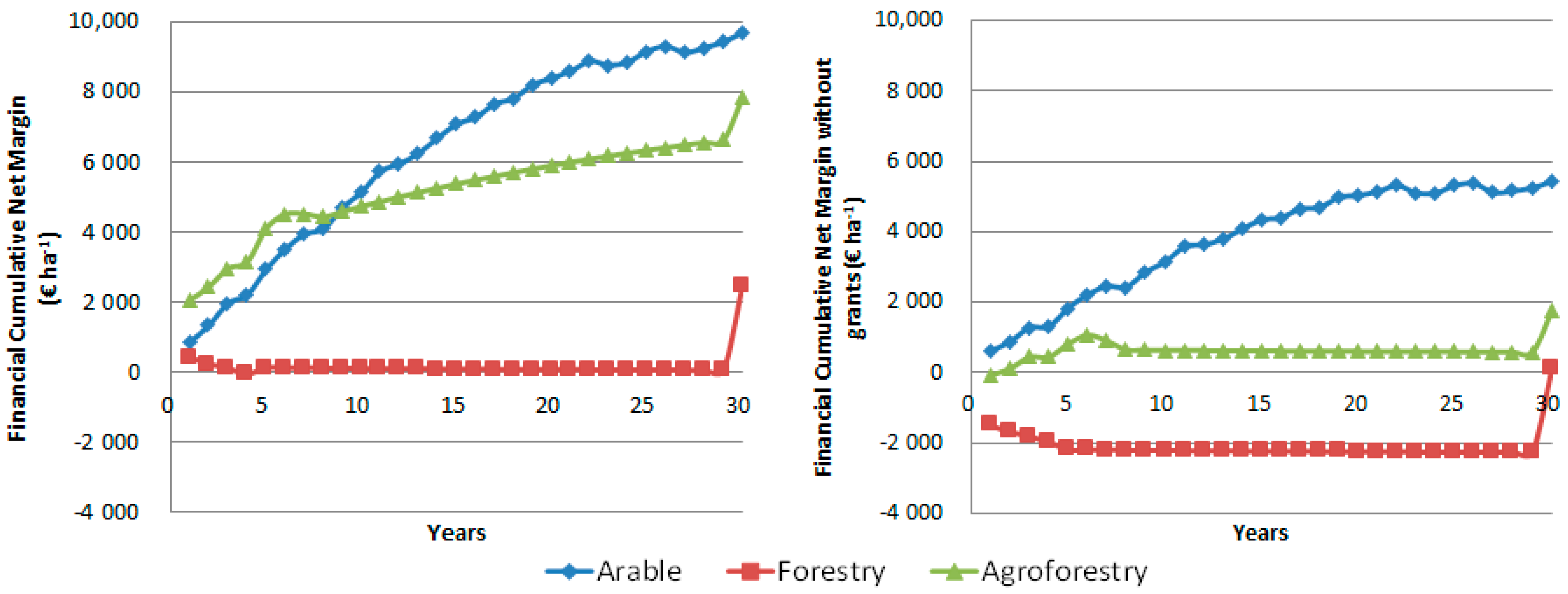
2.3.1. Financial Appraisal

All future costs and benefits were discounted and converted into a financial net present value NPV_F [41] to account for the short- and long-term time preference for money using:

$$NP{V}_F={\displaystyle \sum }_{t=0}^n\left(\frac{\left(B_t-V_t-A_t\right)}{{\left(1+i\right)}^t}\right)$$

(1)

where $B_t$ were benefits, $V_t$ were variable and $A_t$ were assignable fixed costs in year t with a discount rate i [42].

In comparing systems with different rotation lengths, the equivalent annual value (EAV) was calculated based on the infinite net present value, i.e., the net present value defined over an infinite time horizon, in which each replication had a rotation of n years. The financial EAV (units: EUR ha⁻¹ year⁻¹) was defined as:

$$EA{V}_F=NP{V}_F\ast \left(\frac{{\left(1+i\right)}^n}{{\left(1+i\right)}^n-1}\right)\ast i$$

(2)

For the arable system, benefits comprised annual crop revenues and subsidies. Variable costs depended on crop-specific input factors, whereas assignable fixed costs were assumed to be uniform. Due to the spatial adjustment of the area (reduction from 1 to 0.91 ha) assigned to the crop component in the agroforestry system, values were proportionally adjusted. Due to tree and crop competition in the agroforestry system, it was assumed that if the net margin (i.e., the benefits including product revenue and grants minus variable and assignable fixed costs) without grants of the intercrop fell below zero, intercrop production would be suspended and a low productivity non-revenue earning grass sward would be established.

The financial data for the forestry and the tree component of the agroforestry system consisted of revenue from standing timber, government support, and costs for the establishment and maintenance of the trees. The standing value of a cubic metre of timber and the volume of the tree species determined revenues. Firewood was excluded from the analysis as poplar pruning produces limited material and it was assumed the material would decompose or be burnt on site. A grass sward was established on the land in between tree rows.

The time preference of money (present rather than future value) was taken into consideration by applying a discount rate [43]. A discount rate of 4% was assumed to reflect real opportunity costs of capital tied up in the production systems.

2.3.2. GHG Emissions and Sequestration in the Farm-SAFE Model

The Farm-SAFE model was adapted for analysis of environmental burdens associated with GHG emissions and carbon sequestration in above-ground biomass. Farm-SAFE was therefore developed to be able to systematically quantify the energy and resources that were used (inputs) and the emissions that were created and released into the environment (burdens) over the 30-year time horizon [44].

2.3.3. Greenhouse Gas Emissions in the LCA

Here, we focussed on one environmental burden, GHG emissions, since this was the impact category for climate change. This was quantified as a global warming potential (GWP) using conversion factors from [1] (25 for methane (CH₄); 298 for nitrous oxide (N₂O)) to convert non-CO₂ GHG into CO₂e.

The scope was limited to emissions from field-diesel used for machinery operations and direct and indirect N₂O emissions from N inputs, particularly N fertiliser use and nitrate leaching.

A long-term perspective was applied to one full rotation of the perennial woody component (30 years). This long-term perspective assumed a steady state of all mass and energy flows for sustainable agricultural production, ensuring that practices would not allow build-up or depletion of nutrients [25].

A ‘cradle-to-farm gate’ perspective was applied to the arable system. Cooling, drying, storage, and transportation were assumed to take place outside the farm gate and were thus out of scope. The establishment of the farm itself as well as the construction of the farm infrastructure were not included, given their very long-term nature. The land was assumed to be agricultural in previous years, therefore no GHG emissions associated with land use change were assumed to have taken place. Figure 2 illustrates the system boundary for the arable system and highlights the aspects under study.

Figure 2. System diagram for the Life Cycle Assessment (LCA) model integrated in Farm-SAFE to evaluate arable systems. Adapted from Kaske [45].

Figure 2. System diagram for the Life Cycle Assessment (LCA) model integrated in Farm-SAFE to evaluate arable systems. Adapted from Kaske [45].

The system boundary of the forestry system (Figure 3) excludes nursery activities for trees, as poplar has the capability to root from cuttings, when planted directly into the ground [46]. To align the forestry and arable systems, the establishment of a new road network was also excluded from the analysis. The agroforestry system integrates crops and trees, hence the system boundary encompassed both the arable and forestry systems.

Figure 3. System diagram for the Life Cycle Assessment (LCA) model integrated in Farm-SAFE to evaluate forestry systems. Adapted from Kaske [45].

Figure 3. System diagram for the Life Cycle Assessment (LCA) model integrated in Farm-SAFE to evaluate forestry systems. Adapted from Kaske [45].

Inputs of field diesel, fertiliser and pesticides were traced back to their primary resources and the emissions to air were recorded, hence accounting for all upstream impacts. The manufacturing of agricultural machinery was included in proportion to its utilisation rate within the agricultural production system. A delivery distance of 250 km by road was assumed for UK produced items. A weighted average distance was derived for supply chains of phosphate from Tunisia and Morocco [25].

Aboveground-Biomass Carbon Sequestration

Estimates for carbon sequestration in above-ground biomass were obtained from the Yield-SAFE model [35]. Based on the assumption that timber for long-term utilisation could be assigned to carbon stocks, only standing timber was considered and firewood biomass with short-term utilisation was excluded from the analysis. The following three steps were taken to obtain carbon stock estimates that could be used with valuation data that are typically given per tonne CO₂e:

• Conversion of fresh timber volume into dry timber mass. Since the Yield-SAFE model provides timber volume predictions, this needed to be converted into a timber mass. This was done using a wood density value for poplars from Dryad [47] of 0.353 t m⁻³.
• Conversion of dry timber mass into timber carbon. This was done assuming values from Nair [21] and Nair et al. [19] showing that 50% of the mass of timber is carbon.
• Conversion of carbon into CO₂e was done by scaling the molecular mass of carbon dioxide (44) to the atomic mass of carbon (12) in tree biomass. Thus, 1 kg of carbon taken up into biomass is equivalent to an emission of 3.67 kg CO₂e.

2.3.4. Economic Appraisal

The valuation of carbon was based on marginal abatement cost estimates suggested by the Department for Business, Energy & Industrial Strategy [48]. BEIS [48] suggests a range of carbon values (low, central and high) for consideration in project appraisals. The range of central carbon values for the price of carbon was assumed for the economic appraisal; the non-traded price of carbon was used until 2030; a global market price was assumed for post 2030. Over the rotation cycle (2015–2045), the value of CO₂e increased from EUR 14.3 to 90.62. However, this value is not the price that farmers currently receive in the UK. According to the UK Forestry Commission [49], the carbon price was EUR 7.8 per t CO₂e in 2014. For this reason, the economic appraisal was performed using both the central value of carbon suggested by BEIS [48] and the carbon price that was available to landowners under the Woodland Carbon Code in the UK for 2015.

The economic appraisal built upon the NPV_F (see Equation (1)) and included costs for the environmental burden and benefits for carbon sequestration. Hence, the NPV for the economic appraisal (NPV_E) was denoted as:

$$NP{V}_E={\displaystyle \sum }_{t=0}^n\left(\frac{\left(B_t-V_t-A_t\right)}{{\left(1+i\right)}^t}\right)-{\displaystyle \sum }_{t=0}^n\left(\frac{C{E}_t}{{\left(1+j\right)}^t}\right)+{\displaystyle \sum }_{t=0}^n\left(\frac{C{S}_n}{{\left(1+j\right)}^n}\right)$$

(3)

where CE_t is the annual emitted CO₂e in monetary terms and CS_n is the annual sequestered carbon in monetary terms and then discounted to their present values. From the NPV_E, the economic EAV was calculated using Equation (2).

In order to account for future generations and their interests [43], the discount rate for societal costs and benefits j was adjusted from the private market rate. In contrast to the discount rate for private investments, the UK “Green Book” suggested a social time preference rate of 3.5 percent [50].

The inclusion of inventory data within Farm-SAFE allowed labour requirements to be calculated from functions relating to soil type and implement size, for use in the financial appraisal. This drew on the work by Williams et al. [25]. Two carbon values were examined, one using values from the Forestry Commission [49] and one using central carbon prices provided by the UK Department for Business, Energy & Industrial Strategy.

3. Results

3.1. Financial Appraisal

Figure 4 shows the cumulative net margin with and without grants at a discount rate of 4 percent for a cycle of 30 years. The values in the graph in year 30 show the NPV_F. Both with and without grants the three systems showed positive NPV_F. With grants, the arable system had a NPV_F of around EUR 9670 ha⁻¹, the agroforestry system EUR 8360 ha⁻¹, and the forestry system EUR 2440 ha⁻¹. Although forestry was less profitable than arable or agroforestry, the difference in the NPV_F was notably reduced when the grants were excluded from the analysis. This was because cereal farmers in England receive about EUR 235 ha⁻¹ yr⁻¹ under the Single Payment Scheme [36]. For forestry, the only grants considered were payments for tree establishment during the first five years. For agroforestry, it was assumed that farmers would get a pro-rata annual single farm payment for cereal farmers and a pro-rata payment for tree establishment during the first five years.

Without grants, the cumulative net margin of the arable system generally increased during the whole rotation, indicating a constant positive annual net margin (Figure 4), although it is worth noting that in some years, the cumulative net margin dipped, where annual net margins were negative due to poor weather. By contrast, the forestry system did not have a positive cumulative or annual net margin until year 30 when the timber was harvested. As the poplar plantations were planted at final density, there was no intermediate revenue from thinning. In the case of agroforestry, the cumulative net margin increased until year 6, then decreased slightly until year 8 and thereafter remained linear until it increased with the final harvest in year 30. This was in part due to the dynamics of competition for light, nutrients and water between the trees and the crops. As the trees became larger, the Yield-SAFE simulation showed that this would increasingly suppress crop growth, eventually making the intercrop unprofitable. It was therefore assumed that the farmer would stop producing intercrops at some point in the rotation in order to avoid losing future revenue. Here, it was decided that the farmer would stop intercrop and let a low productivity grass cover grow instead, if in three consecutive years, the net margin of the crop component without grants was negative. This assumption is shown in Figure 5, where the evolution of the intercrop net margin in the agroforestry systems without grants over the 30-year rotation is described. Without overriding the decision to plant, the simulation showed that intercrop production would generally be unprofitable from year 11 (grey line). Greater overall profit for the agroforestry system was obtained by halting intercropping and letting a low productivity grass cover establish instead (green line). In this simulation, this point was achieved after three consecutive years of negative net margins between from year 11 to 13.

3.2. GHG Emissions and Carbon Sequestration

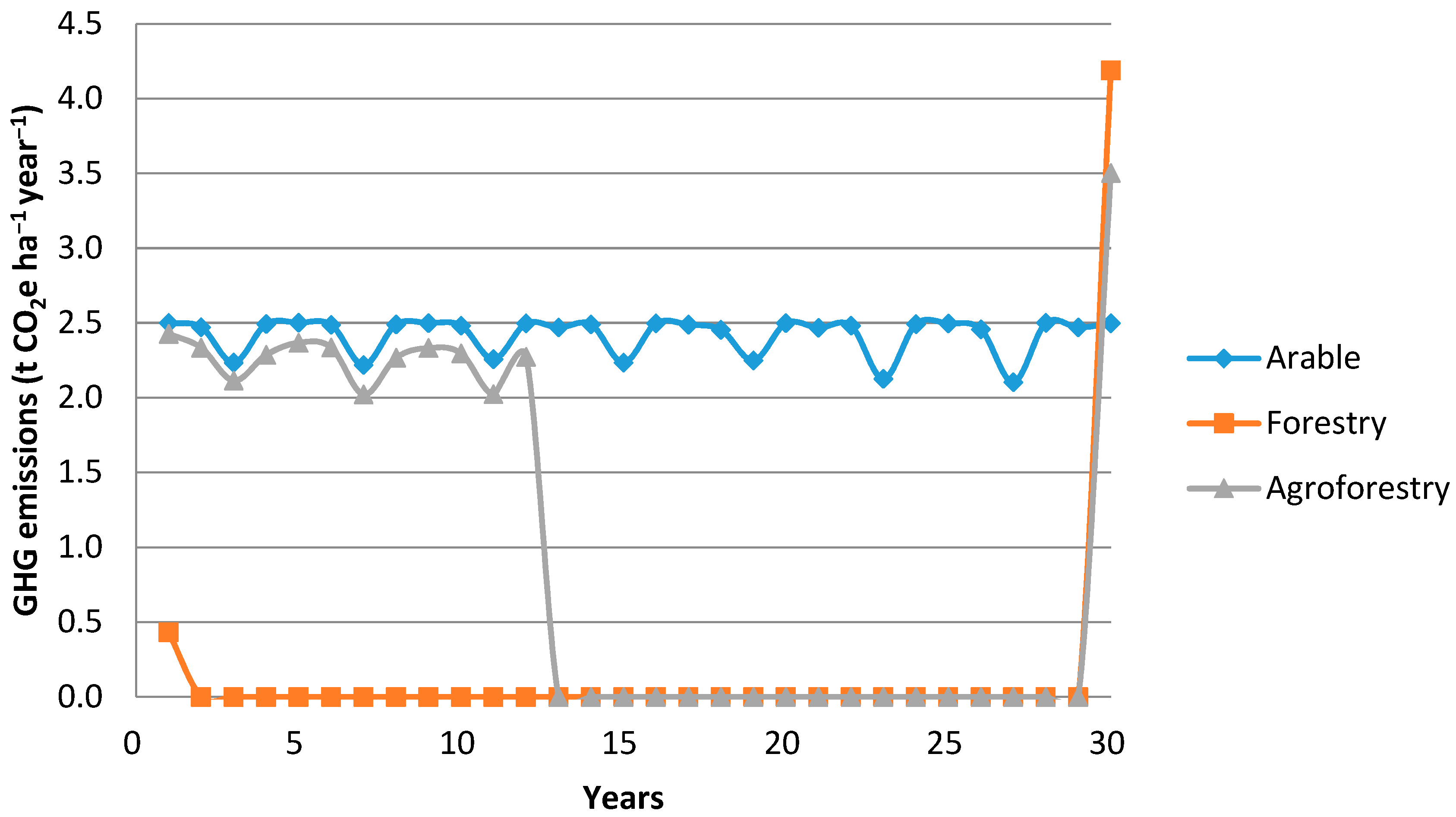
3.2.1. GHG Emissions

In the arable system, the largest proportion of emissions (75%) arose from the manufacture and use of agrochemicals (

Table 1. Mean annual emissions of carbon dioxide equivalent in the LCA of the different production systems. Figures in brackets represent percentages.

On-Field Activity	Arable System	Forestry System	Agroforestry
			Crop	Tree	Combined
	t CO2e ha−1 (%)	t CO2e ha−1 (%)	t CO2e ha−1 (%)	t CO2e ha−1 (%)	t CO2e ha−1 (%)
Cultivation a	0.19 (7.7)	0.01 (7.6)	0.07 (7.4)	0.00 (1.1)	0.07 (6.7)
Agrochemical Application a	0.06 (2.3)	0.00 (0.0)	0.02 (2.3)	0.00 (0.0)	0.02 (2.0)
Harvest and baling a	0.22 (9.1)	0.12 (75.5)	0.08 (8.9)	0.10 (82.3)	0.18 (17.5)
Machinery manufacture	0.15 (6.1)	0.03 (16.9)	0.08 (9.2)	0.02 (16.6)	0.10 (10.1)
Machinery operations (total)	0.61 (25.3)	0.15 (100.0)	0.25 (27.9)	0.12 (100.0)	0.37 (36.3)
Fertiliser b	1.63 (67.3)	0.00 (0.0)	0.58 (64.8)	0.00 (0.0)	0.58 (57.3)
Pesticides c	0.18 (7.4)	0.00 (0.0)	0.07 (7.3)	0.00 (0.0)	0.07 (6.4)
Agrochemicals (total)	1.81 (74.7)	0.00 (0.0)	0.65 (72.1)	0.00 (0.0)	0.65 (63.7)
Combined total	2.42 (100.0)	0.15 (100.0)	0.90 (100.0)	0.12 (100.0)	1.02 (100.0)

^a Fuel use. ^b manufacturing, delivery and field emissions from N fertiliser. ^c manufacturing and delivery, Note: emissions from crop residues are not included as it is assumed straw is collected and sold.

). The use of fertiliser accounted for 1.6 t CO₂e ha⁻¹ yr⁻¹ and constituted 90% of the agrochemical burden and 67% of the overall burden of the arable system (2.42 t CO₂e ha⁻¹ yr⁻¹). There were direct N₂O emissions from N fertiliser use as well as secondary emissions from nitrate leaching and ammonia emissions. The manufacture and use of pesticides summed to 0.18 t CO₂e ha⁻¹ yr⁻¹. Pesticides included manufacture and delivery, but there were no field GHG emissions from pesticide use. Machinery operations (field diesel use and manufacture of tractors and implements) accounted for 25% of the overall burden (0.61 t CO₂e ha⁻¹ yr⁻¹), with 31%, 9%, 36% and 24% of this associated with cultivation, agrochemicals, harvest and manufacture of machinery and storage buildings, respectively. No above-ground crop residues were included as straw was assumed to be harvested and sold.

In contrast, machinery operations in the forestry system accounted for 100% of the total 0.15 t CO₂e ha⁻¹ year⁻¹. These emissions were broken down to harvesting (76%), 7.6% to cultivation and 17% to manufacture of machinery and buildings. The relatively low GHG emission associated with the forestry system were because we assumed that farmers would not apply fertilisers to trees and because of lower levels of machinery use. In addition, pesticides used for localised weeding operations were minimal, and accounted for less than 0.01 t CO₂e ha⁻¹ yr⁻¹ (0.0%).

Total GHG emissions from the agroforestry system were 1.02 t CO₂e ha⁻¹ yr⁻¹, about seven times higher than from forestry, but about 40% of the arable system. Like the arable system, these were dominated by fertiliser manufacture and use (57%) followed by machinery operations (including fuel, manufacture and storage) at 36% and pesticide manufacture at 7%.

Figure 6 shows the annual GHG emissions over the 30-year rotation of the three systems. In the arable system, the difference between years was due to the differences in agrochemical inputs, field operations, and machinery used for the different crop species. With forestry, the emissions were almost negligible, except in year 1, when ploughing and planting were undertaken and in year 30 due to tree felling, loading and transport. Thinning was not assumed in the forestry or agroforestry systems, which were planted at final density. With agroforestry the emissions dramatically declined from year 12 when the crop ceased to be planted, until the machinery operations for the tree harvest in year 30.

3.2.2. Above-Ground Carbon Sequestration and GHG Balance

Figure 7 shows the cumulative CO₂e sequestered in above-ground biomass. As arable crops are harvested annually, the sequestered above-ground CO₂e at the end of the year is considered to be negligible (0 t CO₂e ha⁻¹ yr⁻¹). In contrast, forestry sequestered 260 t CO₂e ha⁻¹ over the 30-year time horizon, averaging 8.73 t CO₂e ha⁻¹ yr⁻¹. Agroforestry sequestered about half as much as forestry at 135 t CO₂e ha⁻¹ (averaging 4.51 t CO₂e ha⁻¹ year⁻¹). The higher tree density in the forestry system compared to the agroforestry system led to higher carbon sequestration of above-ground biomass.

The net GHG balance (

Table 2. Annual GHG emissions, sequestration and equivalent annual value (EAV) at a 3.5% discount rate of an arable, forestry and agroforestry system in England.

Description and Units	Arable	Forestry	Agroforestry
			Crop	Tree	Combined
CO2e Emissions (t CO2e ha−1 year−1)	2.42	0.15	0.90	0.07	0.97
CO2e sequestration aboveground (t CO2e ha−1 year−1)	0.00	8.73	0.00	4.51	4.51
Net balance CO2e (t CO2e ha−1 year−1)	−2.42	8.58	−0.90	4.44	3.54
Financial EAV with grants (EUR ha−1 year−1)	559	141	315	138	453
Financial EAV without grants (EUR ha−1 year−1)	315	9	100	6	106
‘Current carbon price’ scenario [50]
EAV of net balance CO2e (EUR ha−1 year−1)	−19	67	−10	29	20
Economic EAV with grants (EUR ha−1 year−1)	540	208	305	168	473
Economic EAV without grants (EUR ha−1 year−1)	296	76	91	35	126
‘Central carbon price’ scenario [49]
EAV of net balance CO2e (EUR ha−1 year−1)	−287	981	−108	520	412
Economic EAV with grants (EUR ha−1 year−1)	273	1122	207	658	865
Economic EAV without grants (EUR ha−1 year−1)	28	990	−8	526	518

) was calculated on an annual basis as the difference between annual sequestration and annual emissions. The average annual values over the 30-year rotation showed that the net GHG balance was −2.42, 3.54 and 8.58 t CO₂e ha⁻¹ yr⁻¹ for the arable, agroforestry and forestry systems, respectively, illustrating the lack of sequestration in annual cropping.

3.3. Economic Appraisal

The analysis showed that the EAV_F, with grants, for the arable system (EUR 559 ha⁻¹) was more profitable for the farmer than the agroforestry (EUR 453 ha⁻¹) and forestry systems (EUR 141 ha⁻¹). Without grants, the profitability of the agroforestry system (EUR 106 ha⁻¹) was between that for the arable (EUR 315 ha⁻¹) and forestry systems (EUR 9 ha⁻¹). Since grants are paid by society, and are viewed as transfer payments, it can be argued that the societal benefits of the system are best considered without the inclusion of grants.

The economic EAV highlights how including environmental costs can change the relative societal advantage of different land uses. Assuming no grants and using the ‘current carbon price’ scenario, the inclusion of the cost of GHG emissions reduced the difference between the EAV of the arable and the agroforestry system from EUR 209 to 170 ha⁻¹. Under the ‘central carbon price’ scenario, this difference was reduced from EUR 209 ha⁻¹ to EUR −490 ha⁻¹ since the agroforestry system was much more profitable than the arable system under this scenario. This highlights how the inclusion of environmental values within cost-benefit analysis as reflected through different prices can change what is the best solution overall for society.

4. Discussion

The analysis undertaken here showed that the arable system was more profitable than both the forestry and agroforestry systems when compared on a purely financial basis (Financial EAV) both with and without grants. The provision of grants was, however, particularly important for the forestry system and the tree component of the agroforestry system, as without grants, the Financial EAV showed that income would be low. This was a particular challenge for the forestry system without grants and was caused by a combination of the lack of revenue until final harvest and establishment and pruning operations during the early years of the rotation which incurred costs. The inclusion of grants provided some income in the initial years so that the income stream, although relatively low in comparison with the arable and agroforestry system, was positive. In the agroforestry system without grants, the tree management costs were partly offset early in the 30-year cycle by revenue from the crop component. However, when grants were included for the intercrop area, this offsetting effect was much greater, and the agroforestry Financial EAV then was closer to the Financial EAV of the arable system rather than the Financial EAV of the forestry system, as was the case without grants. In both the with and without grant scenarios, and from a perspective that was based purely on financial returns as shown by the Financial EAVs, a farmer presented with a choice between the three systems assessed here would choose the arable system above the agroforestry and forestry systems.

However, the inclusion of a value for carbon, reflecting the broader environmental externalities associated with land use and management, created costs associated with GHG emissions as well as benefits for carbon sequestration. Due to the different inputs and operations associated with arable, forestry, and silvoarable systems, the systems were impacted in different ways. The GHG emissions arising from the inputs and operations associated with the three production systems depressed the Economic EAV of all three production systems. However, the Economic EAV of the arable system was much more severely depressed at both ‘Current carbon price’ and ‘Central carbon price’ scenarios than the tree systems, due to the greater GHG emissions associated with its management. At the same time, for the forestry and agroforestry system, the carbon sequestration associated with tree growth offset the GHG emissions associated with management. Although under the ‘Current carbon price’ scenario (EUR 7.8 t CO₂e⁻¹), the arable system was still more profitable than the forestry and agroforestry systems, under the ‘Central carbon price’ scenario provided by BEIS [48], this resulted in the forestry system becoming more profitable than both the arable and agroforestry systems. In fact, under the ‘Central carbon price’ scenario, the arable system became the least profitable system. Thus, from this perspective, with the assumed prices for inputs and outputs, and the inclusion of GHG emissions and carbon sequestration as externalities of land use choices, the interests of society would best be served through planting of the forestry systems, in preference to both the arable and agroforestry system. This results from the importance placed on improving the climate regulation ecosystem service, as reflected through the value of the ‘Central carbon price’ scenario provided by BEIS [48].

This finding very clearly illustrates the importance of considering environmental externalities in land use options and illustrates the conflicting interests associated with private and public decision-making, where due to the way that property rights are bestowed on individuals (or organisations), land use decisions can be made that benefit individuals and corporate entities at the expense of society as a whole.

In this respect, a range of provisioning, regulating and cultural ecosystem services are provided by the environment, many of which are non-market benefits. Previous research has shown that tree-based systems can provide important benefits relative to arable systems, for example, in terms of regulating ecosystem services (e.g., soil erosion control, nutrient reduction in water, air quality improvement) [51,52] and cultural ecosystem services (e.g., recreation, aesthetics and sense of place) [53,54]. The value of these benefits for society needs to be incorporated in cost-benefit analysis studies to provide an improved basis for valuing land use systems.

Several considerations for future research emerge from this study. In general, LCA data are constantly developing and improving over time, and studies need to be updated to ensure that the LCA studies are accurate and consistent with the latest data and methods of production.

Here, for example, low GHG emissions for the tree component were obtained due to the assumption that labour rather than machinery would be used to manage the poplar trees as they were planted at a relatively low density. However, some studies have found higher GHG emissions associated with mechanised management of woody species [28,29,32] than described here. Whilst detailed comparison with these studies is difficult, since different system boundaries have been used in the different analyses, it is likely that increasing the degree of mechanised work in the management of the trees, particularly because other species may be planted much more densely, or over very large areas where manual labour would become too costly, would increase the per hectare GHG burdens associated with tree management. Further research could be undertaken on these and other commonly used tree species using mechanised systems of management.

In the long term, trees will remove P and K from the soil and sub-soil when the timber is harvested and if not supplied externally will potentially reduce levels in the soil. Tree leaf litter will also decompose and release nitrous oxide into the atmosphere as well as provide organic C to the soil carbon pool. These fluxes need to be accounted for to strengthen understanding of tree related externalities and further research should work towards inclusion of these processes.

Greater carbon sequestration potential may also exist in tree-based systems than quantified under the assumptions made here. For example, a large proportion of above-ground biomass could be used as firewood and this was excluded from the analysis here since it forms a short-term carbon pool. However, firewood has the potential to displace emissions from fossil fuels that are used for heating [55]. Future research could consider this substitution value in the overall set of benefits provided by tree-based systems. Studies have also found that lower fertiliser inputs may be needed in the crop component of agroforestry systems due to the recycling of nitrogen applied to the crop through the leaf biomass of the trees [56,57]. These effects were not included in this study, but benefits could include reduced nitrogen leakage into water bodies, as well as reduced fertiliser inputs into the agroforestry intercrop component.

The analysis here focused primarily on above-ground impacts linked to carbon. However, below-ground carbon in root biomass and the soil plays a vital role in the global carbon cycle [19]. Previous research has shown that between 17–38% of the biomass of a tree may be below-ground [58] and soils that have been under tree cover in the long-term are generally relatively high in carbon [59]. Further research should examine the effect of below-ground carbon sequestration on the GHG balance. In this respect, it is likely that consideration of soil carbon impacts in the economic appraisal would increase the benefits of both silvoarable and forestry system relative to the arable system.

It is worth noting that there are also practices that can be used to increase soil carbon and reduce GHG emissions in arable systems [60] and the implications of these could be examined in terms of their costs and benefits. For example, a large proportion of the GHG emission of the arable system was due to fertiliser manufacture and use, especially ammonium nitrate production which is highly energy intensive [61,62,63]. Changing the composition of fertiliser, by using less ammonium nitrate which could in part be achieved by using urea, could also reduce field GHG emissions. However, the benefit of this would have to be weighed against the associated increase in ammonia emissions that reduce air quality and cause acidification and eutrophication [25].

Other alterations to arable management could include use of reduced tillage and no tillage systems. Williams et al. [25] found that changes in cultivation practices reduced machinery operations for seedbed preparations, but subsequently increased the application rate of pesticides which led to higher environmental burdens from pesticide manufacture. In addition, yields were affected by the change of cultivation method with yield losses of 2% and 4% for reduced tillage and direct drilling cultivation, respectively.

Clearly future modelling for valuation analyses of arable, forestry, and agroforestry systems will need to take the complexity of these various practices, impacts, and interactions into consideration when assessing how production systems and land use decisions can be optimized to improve overall societal welfare.

5. Conclusions

This analysis illustrates the conflict of interest that exists between private and public beneficiaries of land use systems. From a private perspective, it is shown through the financial analysis, that benefits to the individual are greatest from the arable system. However, in the more complete economic analysis, valuation of the GHG emissions and carbon sequestration associated with the three systems demonstrated that from a broader societal perspective, arable systems produced significant negative externalities in the form of GHG emissions, whilst both the forestry and agroforestry systems produced positive externalities in the form of carbon sequestration, making them both, and particularly the forestry system, preferable to the arable system under the ‘Central carbon price’ scenario provided by BEIS [48]. This suggests that society would benefit from greater use of these tree-based systems and that directing resources to ensure the provision of carbon sequestration to combat climate change would be a good use of public resources. Whilst the analysis provided here includes a description of the effects of above-ground carbon sequestration and the associated GHG emissions of machinery and agrochemical use, future research should build on this by providing a fuller analysis of the costs of land use systems on other environmental impacts and management options that are available to farmers. In this respect, future research could account for other impact categories of high importance, such as acidification, eutrophication and emissions to water. The results of this study demonstrated that it is critical to consider the broader impacts of land use system, including not just the impacts of provisioning ecosystem services, as is generally the case, but also regulating and cultural ecosystem services, where tree-based systems can outperform arable systems. Making these greater environmental values explicit through carefully constructed modelling evaluations will provide decision-makers with the appropriate information to ensure that ecosystem services from land use systems reflect broader societal needs.

References

1. IPCC. Climate Change 2014: Synthesis Report. Contribution of Working Groups I, II and III to the Fifth Assessment Report of the Intergovernmental Panel on Climate Change; Core Writing Team, Pachauri, R.K., Meyer, L.A., Eds.; IPCC: Geneva, Switzerland, 2014; p. 151. [Google Scholar]
2. Gilbert, N. One-third of our greenhouse gas emissions come from agriculture. Nat. Cell Biol. 2012. [Google Scholar] [CrossRef]
3. Uphoff, N. Agroecological Approaches to Help “Climate Proof” Agriculture While Raising Productivity in the Twenty-First Century. In Sustaining Soil Productivity in Response to Global Climate Change; Wiley: Chichester, UK, 2011; pp. 87–102. [Google Scholar]
4. Dupraz, C.; Burgess, P.; Gavaland, A.; Graves, A.; Herzog, F.; Incoll, L.D.; Jackson, N.; Keesman, K.; Lawson, G.; Lecomte, I.; et al. SAFE Final Report—Synthesis of the Silvoarable Agroforestry for Europe Project; INRA-UMR System Editions: Montpellier, France, 2005. [Google Scholar]
5. Quinkenstein, A.; Wöllecke, J.; Böhm, C.; Grünewald, H.; Freese, D.; Schneider, B.U.; Hüttl, R.F. Ecological benefits of the alley cropping agroforestry system in sensitive regions of Europe. Environ. Sci. Policy 2009, 12, 1112–1121. [Google Scholar] [CrossRef]
6. Nemecek, T.; Dubois, D.; Huguenin-Elie, O.; Gaillard, G. Life cycle assessment of Swiss farming systems: I. Integrated and organic farming. Agric. Syst. 2011, 104, 217–232. [Google Scholar] [CrossRef]
7. Nemecek, T.; Huguenin-Elie, O.; Dubois, D.; Gaillard, G.; Schaller, B.; Chervet, A. Life cycle assessment of Swiss farming systems: II. Extensive and intensive production. Agric. Syst. 2011, 104, 233–245. [Google Scholar] [CrossRef]
8. Palma, J.; Graves, A.; Bunce, R.; Burgess, P.; de Filippi, R.; Keesman, K.; van Keulen, H.; Liagre, F.; Mayus, M.; Moreno, G.; et al. Modeling environmental benefits of silvoarable agroforestry in Europe. Agric. Ecosyst. Environ. 2007, 119, 320–334. [Google Scholar] [CrossRef] [Green Version]
9. European Commission. EU Greenhouse Gas Emissions and Targets. Available online: https://ec.europa.eu/clima/policies/strategies/progress/monitoring_en (accessed on 26 February 2021).
10. Renzulli, P.A.; Bacenetti, J.; Benedetto, G.; Fusi, A.; Ioppolo, G.; Niero, M.; Proto, M.; Salomone, R.; Sica, D.; Supino, S. Life Cycle Assessment in the Cereal and Derived Products Sector. In Life Cycle Assessment in the Agri-Food Sector; Springer International Publishing: Cham, Switzerland, 2015; pp. 185–249. [Google Scholar]
11. Clay, D.; Ottawa, A.; Flores, L.; Delucco, P.; Kacou, E.; Foster, J.; Baffes, J.; Rajadel, T. Export Crops: Toward a Significant Contribution to Growth. In Breaking the Cycle A Strategy for Conflict—Sensitive Rural Growth in Burundi; Baghdadli, I., Harborne, B., Rajadel, T., Eds.; World Bank Working Paper No. 147; World Bank Publications: Washington, DC, USA, 2008. [Google Scholar]
12. Tilman, D.; Cassman, K.G.; Matson, P.A.; Naylor, R.; Polasky, S. Agricultural sustainability and intensive production practices. Nature 2002, 418, 671–677. [Google Scholar] [CrossRef] [PubMed]
13. Smith, J.; Pearce, B.D.; Wolfe, M.S. Reconciling productivity with protection of the environment: Is temperate agroforestry the answer? Renew. Agric. Food Syst. 2012, 28, 1–13. [Google Scholar] [CrossRef]
14. Thornton, P.K. Recalibrating Food Production in the Developing World: Global Warming Will Change More Than Just the Climate; CGIAR Research Program on Climate Change, Agriculture and Food Security: Wageningen, The Netherlands, 2012; p. 16. [Google Scholar]
15. Aertsens, J.; de Nocker, L.; Gobin, A. Valuing the carbon sequestration potential for European agriculture. Land Use Policy 2013, 31, 584–594. [Google Scholar] [CrossRef]
16. McAdam, J.H.; Burgess, P.J.; Graves, A.R.; Rigueiro-Rodríguez, A.; Mosquera-Losada, M.R. Classifications and Functions of Agroforestry Systems in Europe. In Agroforestry in Europe: Current Status and Future Prospects; Springer Netherlands: Dordrecht, The Netherlands, 2009; pp. 21–41. [Google Scholar]
17. Jose, S. Agroforestry for ecosystem services and environmental benefits: An overview. Agrofor. Syst. 2009, 76, 1–10. [Google Scholar] [CrossRef]
18. Mosquera-Losada, M.R.; McAdam, J.H.; Romero-Franco, R.; Santiago-Freijanes, J.J.; Rigueiro-Rodróguez, A. Definitions and Components of Agroforestry Practices in Europe. In Agroforestry in Europe: Current Status and Future Prospects; Springer Netherlands: Dordrecht, The Netherlands, 2009; pp. 3–19. [Google Scholar]
19. Nair, P.K.R.; Kumar, B.M.; Nair, V.D. Agroforestry as a strategy for carbon sequestration. J. Plant Nutr. Soil Sci. 2009, 172, 10–23. [Google Scholar] [CrossRef]
20. Nair, P.R.; Nair, V.D. ‘Solid–fluid–gas’: The state of knowledge on carbon-sequestration potential of agroforestry systems in Africa. Curr. Opin. Environ. Sustain. 2014, 6, 22–27. [Google Scholar] [CrossRef] [Green Version]
21. Nair, P.K.R. Agroforestry Systems and Environmental Quality: Introduction. J. Environ. Qual. 2011, 40, 784–790. [Google Scholar] [CrossRef] [PubMed] [Green Version]
22. Angus, A.; Burgess, P.; Morris, J.; Lingard, J. Agriculture and land use: Demand for and supply of agricultural commodities, characteristics of the farming and food industries, and implications for land use in the UK. Land Use Policy 2009, 26, S230–S242. [Google Scholar] [CrossRef]
23. Graves, A.R. Bio-Economic Evaluation of Agroforestry Systems for Europe. Ph.D. Thesis, Institute of Water and Environment, Cranfield University, Silsoe, Bedfordshire, UK, 2005. [Google Scholar]
24. Haas, G.; Wetterich, F.; Köpke, U. Comparing intensive, extensified and organic grassland farming in southern Germany by process life cycle assessment. Agric. Ecosyst. Environ. 2001, 83, 43–53. [Google Scholar] [CrossRef] [Green Version]
25. Williams, A.G.; Audsley, E.; Sandars, D.L. Environmental burdens of producing bread wheat, oilseed rape and potatoes in England and Wales using simulation and system modelling. Int. J. Life Cycle Assess. 2010, 15, 855–868. [Google Scholar] [CrossRef] [Green Version]
26. British Standards Institution. PAS 2050—Specification for the Assessment of the Life Cycle Greenhouse Gas Emissions of Goods and Services; British Standards Institution: London, UK, 2011. [Google Scholar]
27. Goglio, P.; Brankatschk, G.; Knudsen, M.T.; Williams, A.G.; Nemecek, T. Addressing crop interactions within cropping systems in LCA. Int. J. Life Cycle Assess. 2018, 23, 1735–1743. [Google Scholar] [CrossRef] [Green Version]
28. González-García, S.; Krowas, I.; Becker, G.; Feijoo, G.; Moreira, M.T. Cradle-to-gate life cycle inventory and environmental performance of Douglas-fir roundwood production in Germany. J. Clean. Prod. 2013, 54, 244–252. [Google Scholar] [CrossRef]
29. González-García, S.; Moreira, M.T.; Dias, A.C.; Mola-Yudego, B. Cradle-to-gate Life Cycle Assessment of forest operations in Europe: Environmental and energy profiles. J. Clean. Prod. 2014, 66, 188–198. [Google Scholar] [CrossRef]
30. Klein, D.; Wolf, C.; Schulz, C.; Weber-Blaschke, G. 20 years of life cycle assessment (LCA) in the forestry sector: State of the art and a methodical proposal for the LCA of forest production. Int. J. Life Cycle Assess. 2015, 20, 556–575. [Google Scholar] [CrossRef]
31. Murphy, F.; Devlin, G.; Mcdonnell, K. Energy requirements and environmental impacts associated with the production of short rotation willow (Salix sp.) chip in Ireland. GCB Bioenergy 2013, 6, 727–739. [Google Scholar] [CrossRef] [Green Version]
32. Murphy, F.; Devlin, G.; McDonnell, K.T. Forest biomass supply chains in Ireland: A life cycle assessment of GHG emissions and primary energy balances. Appl. Energy 2014, 116, 1–8. [Google Scholar] [CrossRef] [Green Version]
33. Rives, J.; Fernandez-Rodriguez, I.; Rieradevall, J.; Gabarrell, X.; Durany, X.G. Environmental analysis of raw cork extraction in cork oak forests in southern Europe (Catalonia-Spain). J. Environ. Manag. 2012, 110, 236–245. [Google Scholar] [CrossRef]
34. Burgess, P.J.; Incoll, L.D.; Hart, B.J.; Beaton, A.; Piper, R.W.; Seymour, I.; Reynolds, F.H.; Wright, C.; Pilbeam, D.J.; Graves, A.R. The Impact of Silvoarable Agroforestry with Poplar on Farm Profitability and Biological Diversity; DEFRA: Silsoe, UK, 2003.
35. van Der Werf, W.; Keesman, K.; Burgess, P.J.; Graves, A.R.; Pilbeam, D.; Incoll, L.D.; Metselaar, K.; Mayus, M.; Stappers, R.; van Keulen, H.; et al. Yield-SAFE: A parameter-sparse, process-based dynamic model for predicting resource capture, growth, and production in agroforestry systems. Ecol. Eng. 2007, 29, 419–433. [Google Scholar] [CrossRef] [Green Version]
36. Agro Business Consultants. The Agricultural Budgeting & Costing Book, 80th ed.; Agro Business Consultants: Melton Mowbray, UK, 2015. [Google Scholar]
37. Savill, P.S. The Silviculture of Trees Used in British Forestry; CABI: Wallingford, Oxon, UK, 1991. [Google Scholar]
38. Morison, J.; Matthews, R.; Miller, G.; Perks, M.; Randle, T.; Vanguelova, E.; White, M.; Yamulki, S. Understanding the Carbon and Greenhouse Gas Balance of Forests in Britain; Forestry Commission Research Report; Forestry Commission: Edinburgh, UK, 2012.
39. Karjalainen, T.; Asikainen, A. Greenhouse gas emissions from the use of primary energy in forest operations and long-distance transportation of timber in Finland. Forestry 1996, 69, 216–228. [Google Scholar] [CrossRef]
40. Graves, A.R.; Burgess, P.J.; Herzog, F.; Palma, J. Farm-SAFE 2006 User Manual; Cranfield University: Cranfield, Bedfordshire, UK, 2006. [Google Scholar]
41. Boardman, A.E.; Greenberg, D.H.; Vining, A.R.; Weimer, D.L. Cost-Benefit Analysis: Concepts and Practice, 4th ed.; Pearson: Upper Saddle River, NJ, USA, 2011. [Google Scholar]
42. Graves, A.R.; Burgess, P.J.; Palma, J.H.N.; Herzog, F.; Moreno, G.; Bertomeu, M.; Dupraz, C.; Liagre, F.; Keesman, K.; van der Werf, W.; et al. Development and application of bioeconomic modelling to compare silvoarable, arable, and forestry systems in three European countries. Ecol. Eng. 2007, 29, 434–449. [Google Scholar] [CrossRef] [Green Version]
43. Campbell, H.F.; Brown, R.P.C. Benefit-Cost Analysis: Financial and Economic Appraisal Using Spreadsheets; Cambridge University Press: Cambridge, UK, 2003. [Google Scholar]
44. Audsley, E.; Alber, S.; Clift, R.; Cowell, S.; Crettaz, P.; Gaillard, G.; Hausheer, J.; Jolliett, O.; Kleijn, R.; Mortensen, B.; et al. Harmonisation of Environmental Life Cycle Assessment for Agriculture; Final Report, concerted action AIR-3CT94-2028; Silsoe Research Institute: Silsoe, UK, 1997. [Google Scholar]
45. Kaske, K.J. Development of An Integrated Economic Model for the Assessment of the Environmental Burden of Arable, Forestry and Silvoarable Systems. Master’s Thesis, Cranfield University, Cranfield, Bedfordshire, UK, 2015. [Google Scholar]
46. Forrest, M. Landscape Trees and Shrubs: Selection, Use and Management; CABI: Oxon, UK, 2006. [Google Scholar]
47. Dryad. Global Wood Density Database; Dryad: Alexandria, VA, USA, 2009. [Google Scholar] [CrossRef]
48. BEIS. Updated Short-Term Traded Carbon Values Used for UK Public Policy Appraisal. Available online: https://www.gov.uk/government/collections/carbon-valuation--2#update-to-traded-carbon-values:-2018 (accessed on 26 February 2021).
49. Forestry Commission. The Woodland Carbon Code. A Buyers’ Guide to Woodland Carbon Units. Available online: https://www.woodlandcarboncode.org.uk/images/PDFs/Woodland_Carbon_Code_BuyersGuide_links.pdf (accessed on 19 September 2020).
50. Treasury, H.M. The Green Book: Appraisal and Evaluation in Central Government; HM Treasury and Government Finance Function: London, UK, 2003.
51. Giannitsopoulos, M.L.; Graves, A.R.; Burgess, P.J.; Crous-Duran, J.; Moreno, G.; Herzog, F.; Palma, J.H.; Kay, S.; de Jalón, S.G. Whole system valuation of agroforestry, arable, and tree-only systems at three case study sites in Europe. J. Clean. Prod. 2020, 269, 122283. [Google Scholar] [CrossRef]
52. García de Jalón, S.; Graves, A.; Palma, J.H.N.; Williams, A.; Upson, M.; Burgess, P.J. Modelling and valuing the environmental impacts of arable, forestry and agroforestry systems: A case study. Agrofor. Syst. 2018, 92, 1059–1073. [Google Scholar] [CrossRef] [Green Version]
53. Kay, S.; Rega, C.; Moreno, G.; den Herder, M.; Palma, J.H.N.; Borek, R.; Crous-Duran, J.; Freese, D.; Giannitsopoulos, M.; Graves, A.R.; et al. Agroforestry creates carbon sinks whilst enhancing the environment in agricultural landscapes in Europe. Land Use Policy 2019, 83, 581–593. [Google Scholar] [CrossRef]
54. Fagerholm, N.M.; Torral, G.; Moreno, M.; Girardello, F.; Herzog, S.; Aviron, P.J.; Burgess, J.; Crous-Duran, N.; Ferreiro-Domínguez, A.R.; Graves, A.; et al. Cross-site analysis of perceived ecosystem service benefits in multifunctional landscapes. Glob. Environ. Chang. 2019, 56, 134–147. [Google Scholar] [CrossRef] [Green Version]
55. Lippke, B.; Oneil, E.; Harrison, R.; E Skog, K.; Gustavsson, L.; Sathre, R. Life cycle impacts of forest management and wood utilization on carbon mitigation: Knowns and unknowns. Carbon Manag. 2011, 2, 303–333. [Google Scholar] [CrossRef]
56. Danso, S.K.A.; Bowen, G.D.; Sanginga, N. Biological nitrogen fixation in trees in agro-ecosystems. Plant Soil 1992, 141, 177–196. [Google Scholar] [CrossRef]
57. Dommergues, Y.R. The Role of Biological Nitrogen Fixation in Agroforestry. In Agroforestry: A Decade of Development; Steppler, H.A., Nair, P.K.R., Eds.; International Council for Research in Agroforestry (ICRAF): Nairobi, Kenya, 1987; pp. 245–271. [Google Scholar]
58. Ahirwal, J.; Maiti, S.K. Carbon Sequestration and Soil CO2 Flux in Reclaimed Coal Mine Land from India. In Bio-Geotechnologies for Mine Site Rehabilitation; Prasad, M.N.V., de Campos Favas, P.J., Maiti, S.K., Eds.; Elesevier: Amsterdam, The Netherlands, 2018; p. 730. [Google Scholar]
59. Lal, R. Forest soils and carbon sequestration. For. Ecol. Manag. 2005, 220, 242–258. [Google Scholar] [CrossRef]
60. Smith, P. Carbon sequestration in croplands: The potential in Europe and the global context. Eur. J. Agron. 2004, 20, 229–236. [Google Scholar] [CrossRef]
61. Jenssen, T.K.; Kongshaug, G. Energy Consumption and Greenhouse Gas Emissions in Fertiliser Production. IFS Proceeding Number 509; The International Fertiliser Society: York, UK, 2003. [Google Scholar]
62. Christensen, B.; Brentrup, F.; Six, L.; Pallière, C.; Hoxha, A. Assessing the Carbon Footprint of Fertiliser at Production and Full Life Cycle, Proceedings International Fertiliser Society 751; International Fertiliser Society: London, UK, 2014; p. 19. [Google Scholar]
63. Hoxha, A.; Jenssen, T.K.; Pallière, C.; Cryans, M. European Emissions Trading Scheme Phase III and the EU Fertiliser Industry, Proceedings International Fertiliser Society 690; International Fertiliser Society: London, UK, 2011. [Google Scholar]
Figure 1. Map showing the location of the case study in Silsoe in southern England.
Sustainability 13 03637 g001
Figure 4. Financial cumulative net margin with grants (left) and without grants (right). Discount rate = 4 percent.
Sustainability 13 03637 g004
Figure 5. Evolution of the net margin (NM) of the crop component of the agroforestry system over the 30-year rotation. The light-grey dashed line shows the crop net margins without grants as crop yields decline due to the increased competition from the trees. The orange line shows the crop net margins without grants when the decision to override the crop planting is taken after negative net margins become increasingly frequent.
Sustainability 13 03637 g005
Figure 6. Annual GHG emissions (t CO2e yr−1) over the 30-year rotation for the arable, forestry and agroforestry systems.
Sustainability 13 03637 g006
Figure 7. Cumulative above-ground C sequestered (t CO2e) in the three systems over a 30-year cycle.
Sustainability 13 03637 g007