
A Green Transportation Planning Approach for Coal Heavy-Haul Railway System by Simultaneously Optimizing Energy Consumption and Capacity Utilization

Abstract
:1. Introduction
1.1. Research Background
- Although a series of automatic management and control platforms has been deployed in the railway system, the existing research still lacks ways of using these data. It is difficult to depict and analyze the distribution of train energy consumption under conditions of varying directions, time periods, and origin and destination, etc.
- The relationship between energy consumption and capacity utilization is difficult to determine, and there is a lack of transportation organization programming techniques that take both into account.
1.2. Research Overview
1.3. Main Article Contributions
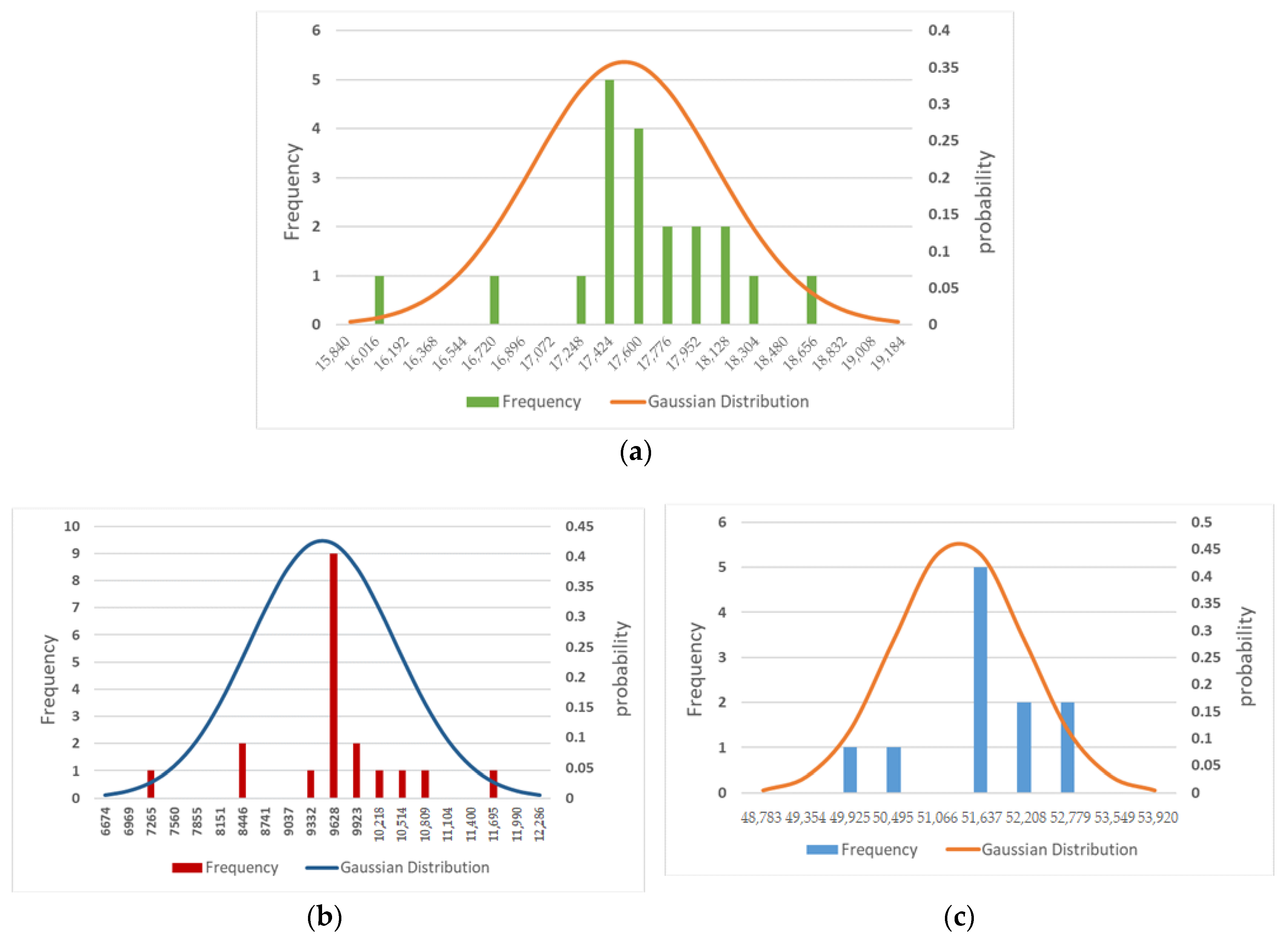
- According to methods based on kinematic theory, an energy consumption calculation approach based on TTD is proposed, then the multidimensional energy consumption values are obtained, which include dimensions such as train forms and routes, etc. In order to solve the problem that the discrete energy consumption value cannot support the requirement of continuity of the objective function in the optimization model, we adopt Gaussian distributions under different dimensions as regression models to fit discrete energy consumption points and construct a distribution model with dimensions for the capacity- and energy-balanced optimization model.
- A simultaneous optimization model for timetable scheduling is proposed, considering objectives including capacity and energy consumption and constraints such as section carrying capacity, station loading and unloading capacity, and station recombination capacity, as well as the different energy consumption characteristics of different train paths. The model is based on a time–space network and the granularity on time can be brought down to 5 min. According to the energy consumption multi-dimensional distribution model, edge weights of the network are set. By means of finding and resolving conflicts in the timetable, we propose a branch-and-bound algorithm to solve the model.
- By comparing and analyzing experiments, some quantitative and qualitative patterns were discovered. This can guide future plan scheduling.
2. Framework and Methods for Energy Consumption Estimation
- (1)
- TTD series data formation. This includes data pre-processing and formatting to time series data.
- (2)
- State-based traction phase detection. This is combined with the transformation method of traction phase identification; the discrete data points in TTD data are transformed into continuous sequence segments.
- (3)
- Noise cleaning of the TTD data for each traction phase. Correction of the data in each traction phase is completed using the Kalman filter.
- (4)
- Energy consumption measurement method based on traction phases. Individual methods for calculating the energy consumption of trains under traction phases are designed.
- (5)
- Multi-dimensional distribution model of energy consumption based on Gaussian distribution. This is based on the assumption of Gaussian distribution. The energy consumption distribution pattern is analyzed and the energy consumption model is established.
2.1. Data Preparation
2.2. Traction Phase Detection
2.2.1. Traction Phases Definition
2.2.2. State-Based Traction Phase Detection Method
| Algorithm 1. Phase detector algorithm. | |
| Input: TTD data DAL_s and level sequence data. | |
| Read TTD data table → DAL_s | |
| Read the sequence of planimetric sections→HoriVert_s | |
| Output: | |
| 1: | Marking train traction phases: Second_Phases→DAL_s [:].phases |
| 2: | Convert consecutive identical point phase codes to linear phase codes (discrete →continuous). |
| 2.1: | |
| 2.2: | Record the position of consecutive identical phase information by differencing the data before and after→pos pos=diff(DAL_s [:].phases) |
| 2.3: | Scan DAL_s, update while DAL_s[pos+1].phases == DAL_s[pos].phases do: = == = |
| 3: | Scanning of horizontal and vertical cross-sectional sequence data, update for i = 1: m do |
| = Func _Height();= Func _Height(); | |
| = Func _Cur (); | |
| Define the elevation function Func _Height, input the coordinates, and output the elevation of the current coordinate. define Func_Height(): | |
| Where HoriVert_s. | |
| return HoriVert_s. | |
| Define the curve function Func_Cur, input the coordinates, and output the curve radius of the current coordinate. define Func_Cur (): | |
| Where HoriVert_s. | |
| return HoriVert_s. | |
2.3. TTD Data Noise Cleaning for Each Traction Phase
| Algorithm 2. Kalman filter algorithm. |
| Input: TTD raw data |
| Read the TTD raw data table→ |
| Output: TTD date DAL_s |
| Save TTD date (DAL_s)→TTD data table |
| If the train traction phases (Phases) is the same as the previous tense |
| 1: Calculate |
| 2: Calculate optimal predictions |
| 3: Calculate the state transfer matrix |
| 4: Calculate the Kalman gain factor |
| 5: Correct best estimate |
| 6: Correct state transfer matrix |
| otherwise |
| 1: |
| 2: Calculat |
| Return , |
2.4. Method of Calculating Energy Consumption for Each Traction Phase
- Acceleration
- 2.
- Coasting
- 3.
- Braking
- 4.
- Total Energy Consumption
2.5. Multi-Dimensional Energy Consumption Distribution Model
3. Optimization Transportation Plans Considering Capacity and Energy Consumption
3.1. Model Building
3.1.1. Notation Definition
3.1.2. Objective Function
- (1)
- The cost of distance traveled by heavy trains is divided into two parts; one is the cost of the actual travel process, and the other is the economic cost of the combined operation.
- (2)
- The energy cost of heavy train transportation is divided into two parts; one is the energy cost spent during the actual travel and the other is the energy cost spent in the combined operation.
- (3)
- The running time span costs accounted for by the train operation plan. The parameter converts the time into other costs by putting energy consumption costs and the travel distance costs on the same scale.
3.1.3. Constraints
- (1)
- Flow balance constraint. For an arbitrary demand , the transport path should be guaranteed to have a beginning and an end, as well as continuity in the path. The following three equations establish the flow balance constraints for the start node, intermediate nodes, and end node, respectively.
- (2)
- Establish a connection between the decision variables y and x. y is used to indicate whether an arc is used or not, and x is used to indicate whether a demand is conveyed by a certain arc.
- (3)
- Train loading capacity constraint. This cannot exceed the number of trains available for supply.
- (4)
- Combination station combination capacity constraint. During any time period, the combination station n completed operations cannot exceed the combination capacity of the station.
- (5)
- The section passing capacity constraint. For any section e, the number of trains released in a given time period cannot exceed the maximum passing capacity constraint of the section.
- (6)
- At a station, only one train can leave at most during a time period.
- (7)
- At a station, only one train can arrive at most during a time period.
- (8)
- Headway time constraint for a combination operation. The necessary time should be left between two adjacent trains for a combination operation, and the waiting time should not be too long.
- (9)
- Total demand constraint. The total amount of actual transportation should be exactly equal to the total amount of demand.
3.2. Branch-and-Bound Algorithm
| Algorithm 3. Branch-and-bound algorithm. | |
| Input: train information weighting factor objective function value factor, set of constraint parameters. | |
| Output: 0–1 decision variables 、, train running plans. | |
| 1: | Create a search space based on the seven dimensions of the variable . |
| 2: | Create a time–space network of railway operations and import information on |
| travel cost , energy cost , interchange cost , etc. | |
| 3: | Simplify the search space into a spatial tree. |
| 4: | Search for a feasible solution using a depth-first search strategy and define as |
| the current initial upper bound. | |
| 5: | Continuing the search for other feasible solutions using a breadth-first search |
| strategy, using the branch-and-bound algorithm. | |
| 5.1 Initialization: number of branches , , 5.2 if if go to 5.2 otherwise go to 5.6 otherwise Take the node with the smallest lower bound value from to become the current expanded node . 5.3 , expand all child nodes of the current expansion node Calculate the lower bound value of each child node , get node Delete the current expansion node 5.4 if All extended child nodes of current node are pruned, , go to 5.2 otherwise go to 5.5 5.5 if Add all nodes to node list Delete all nodes then go to 5.2 otherwise go to 5.6 5.6 if Select the optimal node in the node list to obtain the optimal solution otherwise go to 5.5 end | |
| 6: | After all nodes are searched, the algorithm ends, and the optimal train operation |
| plan is obtained | |
4. Numerical Experiments
4.1. Energy Consumption Calculations and Construction of Multi-Dimensional Distribution Model
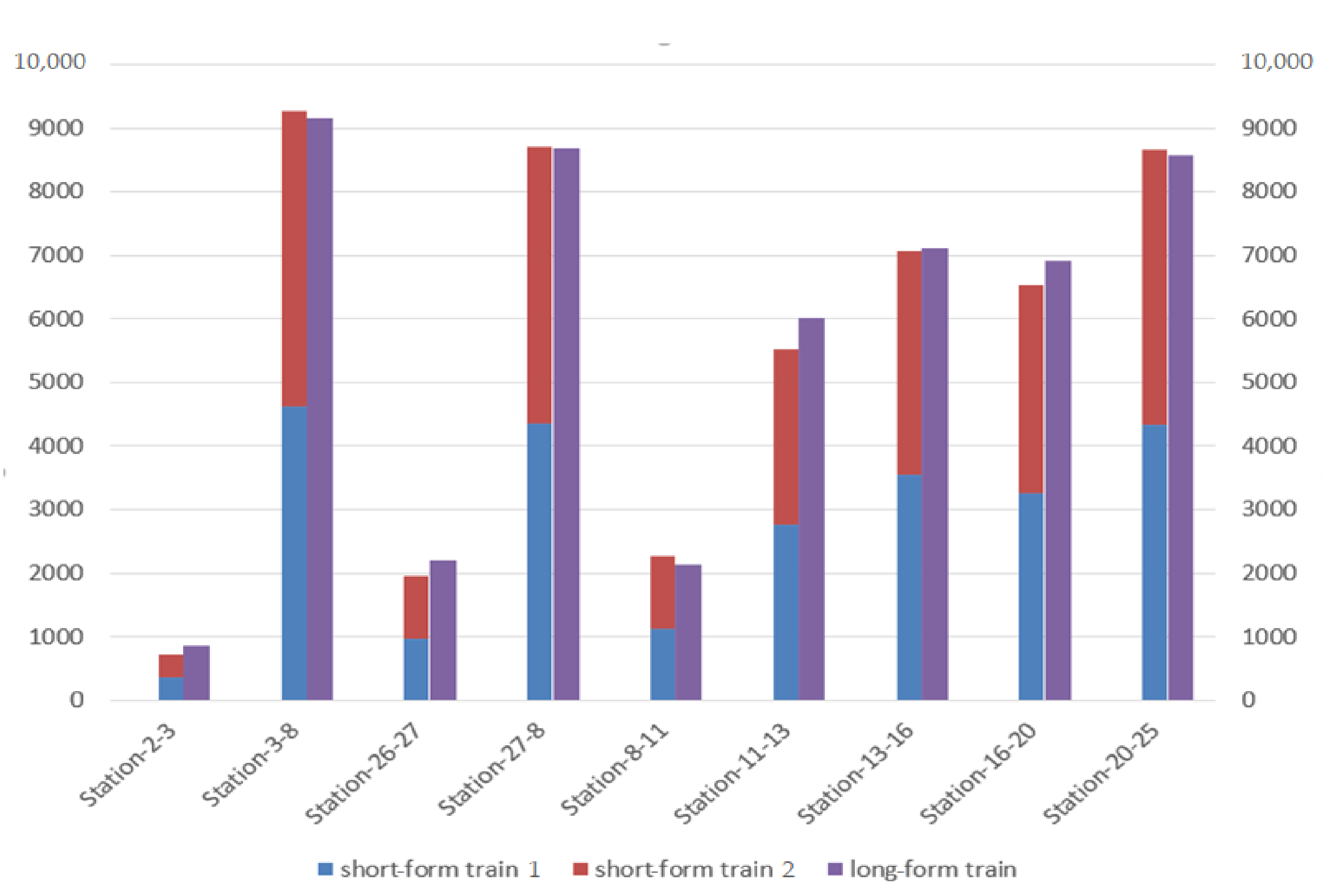
4.2. Comparison of Average Energy Consumption of Long- and Short-Form Trains
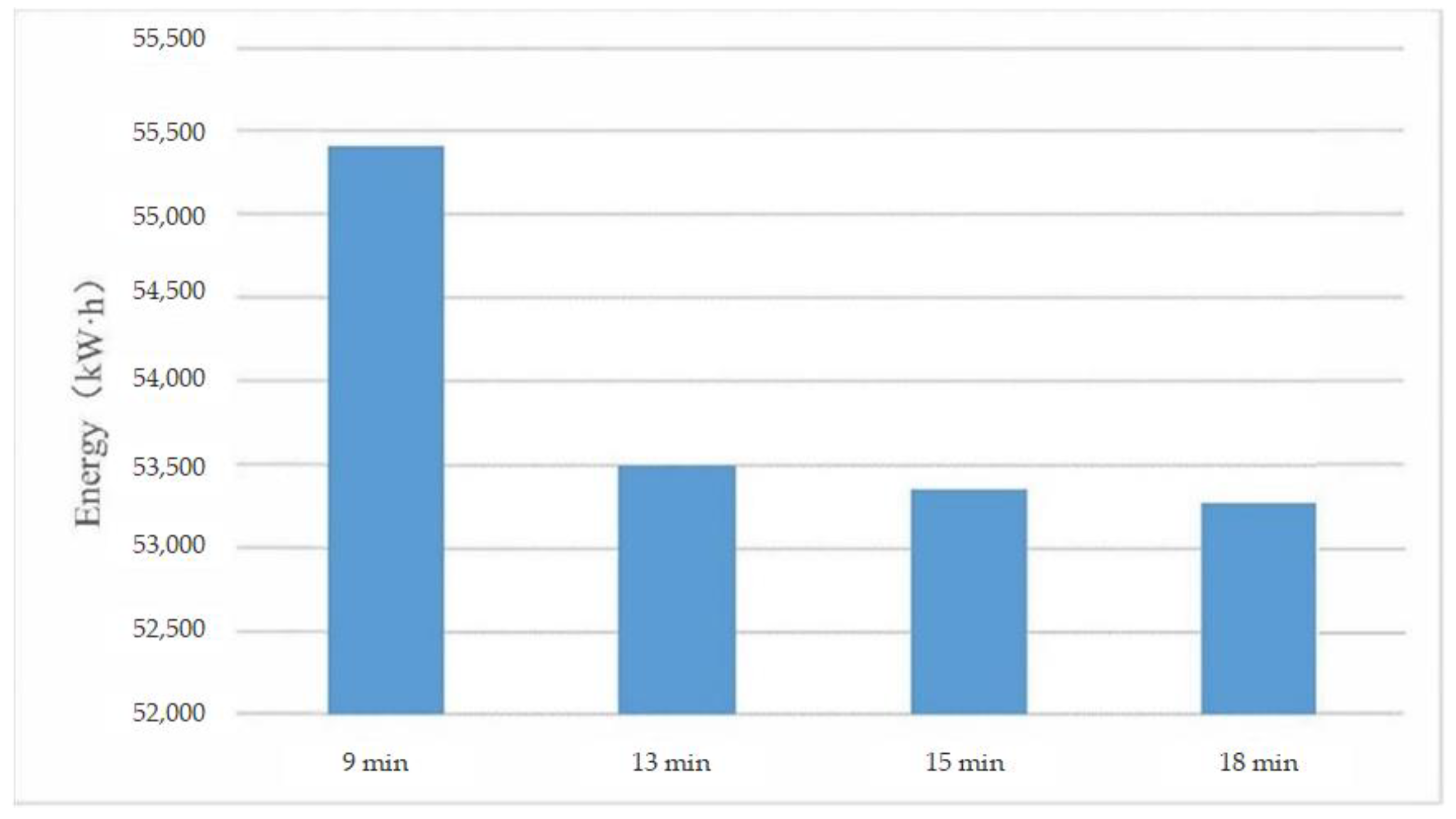
4.3. The Effect of Departure Interval on Energy Consumption of Long Trains
- (1)
- Long-form trains generate more energy consumption when the departure interval is short or in a higher-gradient section. When the departure interval is short or in a higher-gradient section, combining short-form trains into a long-form train will generate more energy consumption (about 5–14% more), although it can improve the traffic density and passing capacity of the section; on the contrary, when the departure interval is long or in a lower-gradient section, a long-form train has a certain advantage in saving energy (about 1–5%).
- (2)
- Compressed departure intervals may cause an increase in energy consumption. For example, when compressing the departure interval of long-form trains, the energy consumption of a 9 min departure interval is higher by 3.6% compared to a 13 min departure interval.
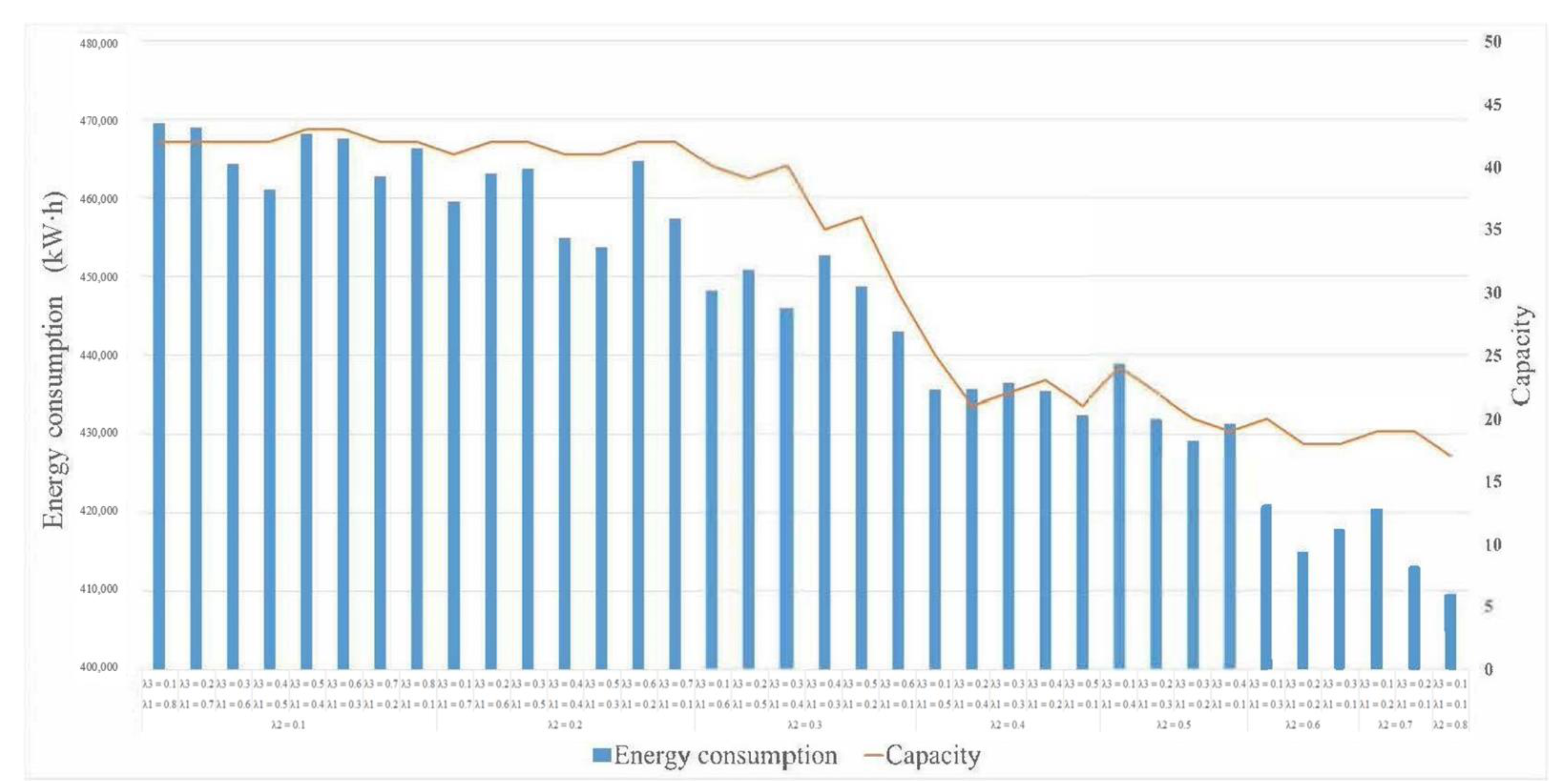
4.4. Analysis of Capacity and Energy Consumption
5. Conclusions
Author Contributions
Funding
Institutional Review Board Statement
Informed Consent Statement
Data Availability Statement
Conflicts of Interest
References
- Assad, A. Analytical models in rail transportation: An annotated bibliography. INFOR Inf. Syst. Oper. Res. 1981, 19, 59–80. [Google Scholar] [CrossRef] [Green Version]
- Assad, A. Analysis of rail classification policies. INFOR Inf. Syst. Oper. Res. 1983, 21, 293–314. [Google Scholar] [CrossRef]
- Bodin, L.D.; Golden, B.L.; Schuster, A.D.; Romig, W. A model for the blocking of trains. Transp. Res. Part B Methodol. 1980, 14, 115–120. [Google Scholar] [CrossRef]
- Kim, N.S.; Van Wee, B. Assessment of co2 emissions for truck-only and rail-based intermodal freight systems in europe. Transp. Plan. Technol. 2009, 32, 313–333. [Google Scholar] [CrossRef]
- Sieminski, A.; Energy Information Administration. International Energy Outlook 2016. Available online: https://www.csis.org/events/eias-international-energy-outlook-2016 (accessed on 12 January 2021).
- Knörr, W.; Seum, S.; Schmied, M.; Kutzner, F.; Anthes, R. Ecological Transport Information Tool for Worldwide Transports—Methodology and Data Update; IFEU: Heidelberg, Germany; INFRAS: Bern, Switzerland; IVE: Hannover, Germany, 2011. [Google Scholar]
- Jorgensen, M.W.; Sorenson, S.C. Estimating emissions from railway traffic. Int. J. Veh. Des. 1998, 20, 210–218. [Google Scholar] [CrossRef]
- Kirschstein, T.; Meisel, F. Ghg-emission models for assessing the eco-friendliness of road and rail freight transports. Transp. Res. Part B Methodol. 2015, 73, 13–33. [Google Scholar] [CrossRef]
- Zhou, X.; Tanvir, S.; Lei, H.; Taylor, J.; Liu, B.; Rouphail, N.M.; Frey, H.C. Integrating a simplified emission estimation model and mesoscopic dynamic traffic simulator to efficiently evaluate emission impacts of traffic management strategies. Transp. Res. Part D Transp. Environ. 2015, 37, 123–136. [Google Scholar] [CrossRef]
- Lindgreen, E.; Sorenson, S.C. Simulation of Energy Consumption and Emissions from Rail Traffic; Technical University of Denmark, Department of Mechanical Engineering: Kongens Lyngby, Denmark, 2005; ISBN 87-7475-328-1. [Google Scholar]
- Patterson, Z.; Ewing, G.O.; Haider, M. The potential for premium-intermodal services to reduce freight co2 emissions in the quebec city–windsor corridor. Transp. Res. Part D Transp. Environ. 2008, 13, 1–9. [Google Scholar] [CrossRef]
- Howlett, P.G.; Pudney, P.J. Energy-Efficient Train Control; Springer Science & Business Media: New York, NY, USA, 2012. [Google Scholar]
- Lukaszewicz, P. Energy saving driving methods for freight trains. Wit Trans. Built Environ. 2004, 74. [Google Scholar] [CrossRef]
- Cortés, C.E.; Vargas, L.S.; Corvalán, R.M. A simulation platform for computing energy consumption and emissions in transportation networks. Transp. Res. Part D Transp. Environ. 2008, 13, 413–427. [Google Scholar] [CrossRef]
- Heinold, A.; Meisel, F. Emission rates of intermodal rail/road and road-only transportation in europe: A comprehensive simulation study. Transp. Res. Part D Transp. Environ. 2018, 65, 421–437. [Google Scholar] [CrossRef]
- Wu, Q.; Spiryagin, M.; Cole, C. Train energy simulation with locomotive adhesion model. Railw. Eng. Sci. 2020, 1–10. [Google Scholar] [CrossRef] [Green Version]
- Drish, W.F., Jr. Train Energy Model—User’s Manual, Version 1.5; Railway Simulators; The National Academies of Sciences, Engineering, and Medicine: Washington, DC, USA, 1989. [Google Scholar]
- Ritzinger, U.; Puchinger, J.; Hartl, R.F. Dynamic programming based metaheuristics for the dial-a-ride problem. Ann. Oper. Res. 2016, 236, 341–358. [Google Scholar] [CrossRef] [Green Version]
- Cucala, A.P.; Fernandez, A.; Sicre, C.; Dominguez, M. Fuzzy optimal schedule of high speed train operation to minimize energy consumption with uncertain delays and driver’s behavioral response. Eng. Appl. Artif. Intell. 2012, 25, 1548–1557. [Google Scholar] [CrossRef]
- Domínguez, M.; Fernández-Cardador, A.; Cucala, A.P.; Gonsalves, T.; Fernández, A. Multi objective particle swarm optimization algorithm for the design of efficient ato speed profiles in metro lines. Eng. Appl. Artif. Intell. 2014, 29. [Google Scholar] [CrossRef]
- Xiang, L.; Hong, K.L. Energy minimization in dynamic train scheduling and control for metro rail operations. Transp. Res. Part B Methodol. 2014, 70, 269–284. [Google Scholar] [CrossRef]
- Chen, D.; Li, S.; Li, J.; Ni, S.; Liu, X. Optimal high-speed railway timetable by stop schedule adjustment for energy-saving. J. Adv. Transp. 2019, 2019, 1–9. [Google Scholar] [CrossRef]
- Zhang, H.; Jia, L.; Wang, L.; Xu, X. Energy consumption optimization of train operation for railway systems: Algorithm development and real-world case study. J. Clean. Prod. 2019, 214, 1024–1037. [Google Scholar] [CrossRef]
- Yang, X.; Chen, A.; Ning, B.; Tang, T. A stochastic model for the integrated optimization on metro timetable and speed profile with uncertain train mass. Transp. Res. Part B Methodol. 2016, 91, 424–445. [Google Scholar] [CrossRef]
- Bocharnikov, Y.V.; Tobias, A.M.; Roberts, C.; Hillmansen, S.; Goodman, C.J. Optimal driving strategy for traction energy saving on dc suburban railways. Iet Electr. Power Appl. 2007, 1, 675–682. [Google Scholar] [CrossRef]
- Yun, B.; Baohua, M.; Fangming, Z.; Yong, D.; Chengbing, D. Energy-efficient driving strategy for freight trains based on power consumption analysis. J. Transp. Syst. Eng. Inf. Technol. 2009, 9, 43–50. [Google Scholar] [CrossRef]
- Xiang, X.; Zhu, X. An optimization strategy for improving the economic performance of heavy-haul railway networks. J. Transp. Eng. 2016, 142, 04016001–04016003.04016013. [Google Scholar] [CrossRef]
- Medanic, J.; Dorfman, M.J. Energy efficient strategies for scheduling trains on a line. IFAC Proc. Vol. 2002, 35, 481–486. [Google Scholar] [CrossRef] [Green Version]
- Albrecht, T.; Oettich, S. A New Integrated Approach to Dynamic-Schedule Synchronization and Energy-Saving Train Control. In Computers in Railways VIII; WIT Press: Southampton, UK, 2002; Volume 61. [Google Scholar]
- Ghoseiri, K.; Szidarovszky, F.; Asgharpour, M.J. A multi-objective train scheduling model and solution. Transp. Res. Part B Methodol. 2004, 38, 927–952. [Google Scholar] [CrossRef]
- Sicre, C.; Cucala, P.; Fernández, A.; Jiménez, J.A.; Serrano, A.A. A Method to Optimise Train Energy Consumption Combining Manual Energy Efficient Driving and Scheduling. In Computers in Railways XII; WIT Press: Southampton, UK, 2010; Volume 114, pp. 549–560. [Google Scholar] [CrossRef] [Green Version]
- Lancien, D.; Fontaine, M. Computing train schedules to save energy: The mareco program. Rev. Gén. Chem. Fer 1981, 100, 679–692. [Google Scholar]


| Scholar | Research Method | Major Contributions |
|---|---|---|
| Cucala [19] Maria [20] | Energy optimization schedule, energy-efficient driving strategies | Integrated optimization of train schedules and driver behavior |
| Xiang L. [21] | Driver behavior analysis | Dynamic train control and driving solution optimization |
| Dingjun Chen [22] | Bi-objective evolutionary algorithm | Establishing an energy-efficient operation diagram for high-speed railways based on stop and dispatch optimization |
| Huiru Zhang [23] | Simulated annealing algorithm | Development of a two-layer planning model for timetable optimization of high-speed rail based on energy-efficient train control |
| Xin Yang [24] | Train operation optimization strategy | Building a comprehensive subway schedule and speed profile optimization model |
| Bocharnikov Y. V. [25] | Trade-off between reduced energy consumption and increased running time to optimize traction energy consumption during a single train run | |
| Bai Yun [26] | Train motion analysis and simulation | Energy consumption at different inertial distances before braking and at lower speed limits, as well as uniformity of train speed |
| Xiang X. [27] | Bi-level algorithm | Selecting the optimal solution set with the lowest total cost under various constraints |
| Dorfman [28] | Scheduling management strategy | For single-track train control issues Using discrete event dynamic systems theory |
| Albrecht [29] | A new approach to integration | Balancing simultaneity and energy efficiency in train schedules |
| Ghoseiri [30] | Multi-objective train optimization mode | Train control that takes into account both train energy consumption and customer travel time |
| Li [21] | Multi-objective train scheduling model | Integrating goals for energy efficiency, emissions reduction, and travel time |
| Sicre [31] | Simulation model to optimize energy consumption | 30% energy saving by using existing simulation platform to optimize train schedules |
| Lancien [32] | Data mining and optimization model | Aiming to minimize energy consumption of trains under fixed service time conditions |
| Notation | Descriptions |
|---|---|
| Original format TTD (train trajectory data) data | |
| -th moment | |
| Train position at time i-th | |
| Train speed at time i-th | |
| Locomotive display at time i-th | |
| Raw elevation data (spatially sequential) | |
| Raw curve radius data (spatially sequential) | |
| Level cross-sectional data (time series) | |
| Data points of the longitudinal and cross sections at moment i | |
| Kilometer marker at the end of the train’s operating segment | |
| The elevation at which the train is located at the moment of i | |
| The radius of the curve where the train is located at moment i | |
| Kind of phase | |
| Basic resistance of heavy vehicle units | |
| Basic resistance of locomotive units | |
| Curve unit basic resistance (N/KN*degree) | |
| curvature | |
| Supply voltage | |
| Self-contained electric current | |
| Motor conversion efficiency | |
| Gross train weight | |
| Locomotive quality | |
| The amount of elevation change before and after a traction phase sequence | |
| Instantaneous velocity before a traction phase sequence | |
| Instantaneous velocity after a traction phase sequence | |
| Mileage position at the start of a traction phase sequence | |
| End-mile position of a traction phase sequence | |
| Information on train operation under different phases | |
| Train departure stations | |
| Train terminal | |
| Train departure time | |
| Final train arrival time | |
| Train traction constant | |
| Different train stop schemes | |
| Train running speed | |
| Energy consumption data for specific train operations under defined conditions |
| Train Status Information | Traction Phases |
|---|---|
| Acceleration is positive and the engine is revving. | Acceleration |
| The engine is not revving and the duct pressure is high. | Coasting |
| The engine is not revving and the duct pressure is low. | Braking |
| Notation | Descriptions |
|---|---|
| Station collection, indexed as i, j, n. | |
| Assembly of combination stations. | |
| Collection of sections in track. | |
| A collection of transportation requirements which, for each requirement, contains the starting station i and the ending station j and the corresponding sequence number k, . | |
| A collection of train services at the service level; each service contains , which are the start station, end station, start time, and end time, respectively. | |
| Waiting arc planning at the demand level, including waiting for loading and waiting for unloading. | |
| Dwell arc after loading at the demand floor, dwell arc after changing trains at the combination station, etc. | |
| Demand layer interchange arcs for two successive train services at the combination station. | |
| The sum of all arcs in the requirements and service layers, A = , where a is the index variable of the arc set. | |
| Represent the out-arc and in-arc sets of all time nodes of node n, separately. | |
| Represent the set of out-arc and in-arc nodes n at time t, separately. | |
| The demand between each demand loading and unloading node is divided into a set of unit volumes, with k as its index variable. | |
| Total coal demand from i to j. | |
| Whether the kth branch of demand between I and j is successfully shipped, if so, = 1, otherwise =0. | |
| Passing capacity as arc e. | |
| The loading capacity of train s, with a value of 1 or 2, representing the short-form train and long-form train, respectively. | |
| The node in time between i and j when the coal demand is ready to be loaded and shipped at any time, with the ability to ship at each integer. | |
| Denotes the average transport time of this tributary (i, j, k). | |
| The arc a in the time–space network is denoted by (), and the five symbols in parentheses denote the original station, destination station, departure time, arrival time, and train properties of the arc, respectively. | |
| Run segment, denoted by . | |
| Maximum combined capacity of combined station n per unit time (time window). | |
| 0–1 associated variable, with a value of 1 if t of the physical segment is passed by the train service arc =1, otherwise =0 | |
| The arc is the cost of running the train in service, | |
| Arc is the interchange cost for combined station transfers. | |
| Arc is the energy cost of the service train. | |
| Arc is the interchange energy cost for the combined station transfer. | |
| Conversion factor per unit of time to other costs. | |
| 0–1 decision variable, if = 1 and , then it means that train service is used; if , then it means that commutation arc is used; otherwise = 0. | |
| 0–1 decision variables, representing the demand generated at moment t from i to j numbered k by train service transport then =1, otherwise =0. |
| Train Form | Number of Stops | OD (Volume from Origin to Destination) | |||
|---|---|---|---|---|---|
| Empty train | 0 | Station 24–Station 2 | 9479.9 | 935.3 | 0.82 |
| Empty train | 0 | Station 24–Station 4 | 8310.4 | 798.4 | 0.84 |
| Empty train | 2 | Station 24–Station 3 | 8942.6 | 872.5 | 0.77 |
| Empty train | 3 | Station 3–Station 24 | 9067.4 | 901.9 | 0.74 |
| Short-form train | 3 | Station 24–Station 2 | 17,981.5 | 1256.4 | 0.73 |
| Short-form train | 3 | Station 25–Station 2 | 18,513.8 | 1174.7 | 0.69 |
| Short-form train | 4 | Station 25–Station 2 | 19,012.4 | 1298.2 | 0.81 |
| Short-form train | 0 | Station 2–Station 24 | 17,512.0 | 557.3 | 0.79 |
| Short-form train | 3 | Station 2–Station 25 | 18,513.7 | 884.2 | 0.73 |
| Long-form train | 0 | Station 2–Station 24 | 51,351.6 | 856.17 | 0.82 |
| Long-form train | 4 | Station 2–Station 24 | 56,922.2 | 1679.8 | 0.87 |
| Long-form train | 4 | Station 4–Station 25 | 55,848.2 | 1567.2 | 0.74 |
| Long-form train | 0 | Station 4–Station 24 | 51,480.9 | 1351.5 | 0.77 |
| Long-form train | 2 | Station 11–Station 24 | 34,047.8 | 1058.6 | 0.75 |
| Section | Short-Form Train 1 | Short-Form Train 2 | Long-Form Train | Proportion |
|---|---|---|---|---|
| Station 2–Station 3 | 367.6 | 367.6 | 860 | −14.51% |
| Station 3–Station 8 | 4633.63 | 4633.63 | 9150 | 1.28% |
| Station 26–Station 27 | 978.52 | 978.52 | 2201 | −11.08% |
| Station 27–Station 8 | 4359.05 | 4359.05 | 8690 | 0.32% |
| Station 8–Station 11 | 1134.04 | 1134.04 | 2145 | 5.74% |
| Station 11–Station 13 | 2759.94 | 2759.94 | 6027.32 | −8.42% |
| Station 13–Station 16 | 3539.78 | 3539.78 | 7120 | −0.57% |
| Station 16–Station 20 | 3265.2 | 3265.2 | 6912 | −5.52% |
| Station 20–Station 25 | 4333.01 | 4333.01 | 8573 | 1.09% |
Publisher’s Note: MDPI stays neutral with regard to jurisdictional claims in published maps and institutional affiliations. |
© 2021 by the authors. Licensee MDPI, Basel, Switzerland. This article is an open access article distributed under the terms and conditions of the Creative Commons Attribution (CC BY) license (https://creativecommons.org/licenses/by/4.0/).
Share and Cite
Fu, J.; Chen, J. A Green Transportation Planning Approach for Coal Heavy-Haul Railway System by Simultaneously Optimizing Energy Consumption and Capacity Utilization. Sustainability 2021, 13, 4173. https://doi.org/10.3390/su13084173
Fu J, Chen J. A Green Transportation Planning Approach for Coal Heavy-Haul Railway System by Simultaneously Optimizing Energy Consumption and Capacity Utilization. Sustainability. 2021; 13(8):4173. https://doi.org/10.3390/su13084173
Chicago/Turabian StyleFu, Jianjun, and Junhua Chen. 2021. "A Green Transportation Planning Approach for Coal Heavy-Haul Railway System by Simultaneously Optimizing Energy Consumption and Capacity Utilization" Sustainability 13, no. 8: 4173. https://doi.org/10.3390/su13084173