Article

Population Density or Populations Size. Which Factor Determines Urban Traffic Congestion?

1
Department of Business, Gachon University, Seongnam 13120, Korea
2
Endicott College of International Studies, Woosong University, Daejeon 34000, Korea
3
Department of Korean Literature & Literature, Gachon University, Seongnam 13120, Korea
*
Author to whom correspondence should be addressed.
Sustainability 2021, 13(8), 4280; https://doi.org/10.3390/su13084280
Submission received: 10 March 2021 / Revised: 8 April 2021 / Accepted: 8 April 2021 / Published: 12 April 2021

Abstract

:
A large number of articles have documented that as population density of cities increases, car use declines and public transit use rises. These articles had a significant impact of promoting high-density compact urban development to mitigate traffic congestion. Another approach followed by other researchers used the urban scaling model to indicate that traffic congestion increases as population size of cities increases, thus generating a possible contradictory result. Therefore, this study examines the role of both density and population size on traffic congestion in 164 global cities by the use of Stochastic Impacts by Regression on Population, Affluence and Technology model. We divide 164 cities into the two subgroups of 66 low density cities and 98 high density cities for analysis. The findings from the subgroups analysis indicated a clear-cut difference on the critical role of density in low-density cities and the exclusive role of population size in high-density cities. Furthermore, using threshold regression model, 164 cities are divided into the two regions of large and small population cities to determine population scale advantage of traffic congestion. Our findings highlight the importance of including analysis of subgroups based on density and/or population size in future studies of traffic congestion.

1. Introduction

Traffic congestion in large global cities continues to worsen resulting in high economic cost, lost time, accidents, pollution, and many other negative effects for billions of urban inhabitants [1,2,3,4]. Research on the causes and mitigation of traffic congestion has produced a very large number of publications particularly over the last three decades [5,6]. The two best known papers, by Newman and Kenworthy (1989) and Kenworthy and Laube (1999), have found a negative correlation between traffic congestion and population density [7,8]. They also found a positive correlation between density and transit use. In other words, high density in cities may discourage car ownership in favor of using public transportation systems. High-density cities may also require shorter driving distances.
Numerous follow-up studies using aggregate or disaggregate samples of cities have had a significant impact of promoting high–density compact urban development to mitigate traffic congestion and pollution. Using an aggregate sample allows the researcher to analyze the overall pattern of traffic congestion for all cities in one sample without differentiating heterogeneous characteristics such as density, population, and income. An aggregate sample can also be categorized into several disaggregate samples of cities with homogeneous characteristics such as density and population. Analysis of disaggregate samples often yields results that may be more relevant to individual cities with unique characteristics.
As for the key determinant of traffic congestion, a common approach is to use population density of a city while another approach is to use population size. Using density as the key determinant often has revealed a negative relationship between traffic congestion and density of cities [7,8]. In contrast, using population size as the key determinant has often shown a positive relationship between congestion and population size of cities. Similarly, using an aggregate versus disaggregate sample often has provided contradicting evidence on the relationship between traffic congestion and cities. This research attempts to resolve these contradictory results by using both aggregate and disaggregate samples of cities. In other words, both population density and population size are used simultaneously as the key determinants of traffic density.
We used traffic congestion data available from TomTom [9]. TomTom [9] created the traffic index (TI) in 2012 to provide an annual benchmark, making it possible to evaluate congestion levels globally in an objective way. In TI 2017, coverage was extended to 390 cities in 48 countries over six continents. Congestion levels are measured as the percentage of increase in overall travel times compared to non-congested, free-flow travel time. For example, a congestion level of 50% means that overall travel time is 50% greater than free-flow travel time. According to Cohn [10], travel times are calculated on all road segments in the top five functional road classes in each urban area. The overall TI value for a city is the weighted average percentage of extra travel time for drivers in that city over 24 h, 7 days a week for the given calendar period. The TI includes 164 large global cities with complete data on the traffic congestion index, population, income per capita, and population density.
A sample of 164 cities obtained from the TI from TomTom will be divided into two disaggregate samples: (1) 66 U.S.-Canadian low-density cities and (2) 98 high-density cities in 14 countries primarily in Europe. We used a cross-sectional multivariate regression model with population size, population density, and income as independent variables. We also examined the population scaling advantage of traffic congestion between the subgroup of large population size cities versus the subgroup of small population size cities. The threshold regression model was used to divide 164 cities into 46 cities whose population size was larger than the threshold value and 118 cities whose population size was less than the threshold value.
This remainder of this paper is organized into four sections. Section 2 is a brief literature review on urban congestion in relation to vehicle and transit usage. The data and method of analysis are presented in Section 3, followed by an analysis of results in Section 4. Finally, conclusions, implications, and limitations of this research are presented in Section 5.

2. Literature Review

2.1. Aggregate and Disaggregate Analysis of Traffic Congestion

The relationship between urban form and traffic congestion or congestion-generated pollution has been studied extensively over several decades, specifically after the publication of two well-known aggregate studies by [7] and [8]. With an aggregate sample of 46 global cities from several regions including North America., Asia, and Europe, Kenworthy and Laube [8] confirmed the earlier finding that as population density increases, car use declines (R2 = 0.838) and transit use rises (R2 = 0.757). These two papers have prompted numerous follow-up studies using both aggregate and disaggregate samples of cities and have had a significant impact of promoting the concept of high-density compact development to mitigate car use, traffic congestion, and pollution. Representative survey articles include [5,11].
Two methods of analysis have been used in traditional aggregate studies. The first group of articles continue to use population density as the key determining factor in multivariate regression analysis. For example, Karathodorou et al. [12] and Sue [13] have found statistically significant negative density coefficients of −0.229 and −0.064, respectively, for fuel consumption, supporting the earlier findings by Newman and Kenworthy [7]. They determined that a 1% increase in density is expected to decrease car fuel consumption by 0.229% and 0.064%, respectively, all else being equal. Ye et al. [14] and Gudipudi et al. [15] also supported the impact of city density on decreased car use and less carbon emissions.
The second aggregate approach uses the urban scaling model, which states that traffic congestion, car use, and pollution emissions may be described by a power-law function [16,17]. For 942 U.S. urban centers, Fragkias et al. [18] established a power function exponent of 1.0 for CO2 emissions as a function of population size, indicating a constant return to scale. In contrast, Oliveira et al. [19] found that the population size to scale superlinearly (with an exponent of 1.46) represented an increasing return to scale when the U.S. cities were defined as connected urban spaces. Muller and Jha [20] found a sublinear exponent of 0.75 for local air pollution for U.S. metropolitan areas, indicating a decreasing scale trend.
For traffic congestion, Louf and Barthelemy [21] derived a population exponent of 1.27 for a variation of total delay hours due to congestion and 1.262 for excess CO2 emissions due to congestion for 101 U.S. cities. Barthelemy [22] also established a scale exponent of 1.58 (r2 = 0.96) for total delay from congestion during peak hours as a function of population size of cities. Barthelemy’s [22] data on almost 300 urban areas globally came from TomTom in 2016.
Kenworthy and Laube’s [8] aggregate study did not explicitly pursue the possibility that driving behavior of people in dense cities may be different from those in less dense cities, even though their data supported this possibility. Their sample of 13 U.S. and 11 European cities clearly showed that the 1990 average density of the European subgroup was about 3.5 times higher at 49.9 persons per hectare and just 14.2 in the North American subgroup. In contrast, the average car use in the North American subgroup is almost 2.5 times higher at 11,155 km per capita and just 4517 for the European subgroup. The difference in driving behavior in cities with different density has been subjected to rigorous quantitative analysis in the context or residential self-selection of driving in disaggregated studies, which we elaborate on next.
One group of disaggregate studies continues to use density as the key determinant. These studies use household data to control for observable driving differences between households living in low- and high-density areas [23,24,25,26]. For example, Brownstone and Golob [25] found that residential density influences car use. Comparing two households that are similar in all aspects except residential density, a lower density of 1000 housing units per square mile, which is about 40% of the mean value of 2500 housing units, implies a positive difference of 1200 miles per year or 4.8% more miles. Duranton and Turner [26] also found that a 10% increase in “residential density” leads to a 0.7% to 1% decline in driving, when the effects from other variables are held constant. “Residential density” is defined as the density of residents and jobs within a 10-km radius of where a driver lives. Other measures of urban form do not have a measurable effect on driving behavior. Policy implications from these studies suggest that it would be more costly to reduce the driving difference through a densification process than through congestion pricing or increased gasoline taxes.
The second group of disaggregate studies has used population as the key determinant. For example, Chang et al. [27] compared a group of cities with less than 1 million inhabitants to show a strong superliner scale at the exponent of 1.7, while another group of cities with more than 3 million inhabitants showed a linear scale at an exponent of 1.0. Lu et al.’s [28] disaggregate study on pollution concluded that the rate of population growth can aggravate air pollution, but the impact is heterogenous. In mega cities, the rate of population growth can improve air quality, and in small- and medium-size cities, the rate of population growth can aggravate air pollution.
Finally, in an attempt to combine both population size and density to examine the effects on urban CO2 emissions, Ribeiro et al. [29] proposed a generalized logistic model. The model can generate decreasing or increasing returns to scale, but population size always has a greater effect on emissions than population density. They also suggested a possible use of the IPAT model, which can use both population size and density simultaneously as predictors.

2.2. Comparison of Transit Capacity and Usage: The U.S. versus Europe

We analyzed the data by separating into two groups: 66 North American (Canada and the United States) cities and 98 other (mostly, European) cities. Separating into two groups in our analysis is based on the expectation that the effect of the independent variable (dense, population, & income) on the dependent variable would be different between the groups.
The primary factor that moderates the effects of independent variables on the dependent variable is public transit system [30]. In general, it is known that there is a strong correlation between population density and transit system usage. However, high density does not necessarily result in increases in transit capacity and transit uses. Well established transit system is expected to mitigate the effects of density, population size, and income on traffic congestion by absorbing the demands for automobile uses. There are sufficient evidences that in the US cities transit capacities and uses are significantly lower than in European cities.
Comparing the differences of transit capacity and transit usage between the 11 metropolitan cities in Europe versus 13 metropolitan U.S cities, Kenworthy and Laube [8] demonstrated a much greater transit dependency of the European cities over the U.S cities. As Table 1 shows, the overall transit capacity measured as transit service kilometers (km) per person was 3.28 times longer at 92 km in the European cities over 28 km in the American cities.
The transit service km per person includes rail service km as well. The rail service intensity measures as rail service km per urban hectare (ha) shows even a greater difference. The European cities experienced 23.86 times higher intensity at 3651 km over just 153 km in the U.S. cities. As for actual passenger travel using transit systems, the European cities captured even a greater proportion of 22.6% over a tiny 3.1% realized by the U.S. cities, which represented 7.27 times higher transit usage by the European cities. Another transit usage measure is percentage of commuting workers using transit during peak hours. Once again, 38.8% of commuters used transit systems in the European cities over just 9.0% in the U.S. cities representing 4.31 times higher usage in the European cities. In short, the transit dependence of the European cities is much greater than the U.S. cities, whereas the automobile dependence is dominant in the U.S. cities.
A discrepancy in dependency on transit systems between the US and European cities has been widen. For example, Freemark [31] in his comparison analysis with data of 2002–2018 period reported that the transit ridership in the U.S. urban cities had declined by 15% during 2010–2018 while that in the French counterparts had increased by 18% during same period of time. With a few exceptions such as New York, Boston, and Houston, people in the U.S. cities tend to prefer using their own cars instead of using public transit system. Freemark [31] attributes the transit’s decline in the U.S. to some factors such as low gas price, cultural influences, and economic differences from European ones. On the contrary, the largest French cities had developed effective tram and bus services. Public transit systems in French cities were designed to serve large and dense cities and a large amount of resources has been invested to develop pedestrian-friendly facilities. As an additional evidence, Figure 1 shows that there is a clear demarcation between US and Western European cities in terms of transit ridership per capita [32].

3. Method and Data

Ribeiro et al. [29] suggested that the well-known environmental principle of I = PAT might be used as the analytical model [33,34,35]. The IPAT (I = PAT) model is a multiplicate approach to assess the role of population (P), affluence (A), and technology(T), on environmental impact (I). The model is not an equation but rather an identity. The IPAT is still useful in determining which factors (driving forces) are most damaging to the environment.
The IPAT model was extended into the stochastic impacts by regression on population, affluence and technology (STIRPAT) model which enabled to estimate the proportional change in environmental impact per given proportional change in population.
The STIRPAT model is defined as
I i = a P i b A i c T i d e i
where a is a constant, b c, and d are the exponents of P, A and T, respectively, that are to be estimated and e is the residual or error term. Subscript i denotes the cross-sectional units, namely cities in this paper.
To ease the task of estimating exponents, Equation (1) is converted into is log-log form of Equation (2) by taking the natural log of both sides.
l n I i = l n a i + b l n p i + c [ l n ( A i ) ] + d [ l n ( t i ) ] + e i
The natural log is helpful as it converts non-linear variables to linear ones rendering the results to interpret as percentage change. For example, b can be viewed as population elasticity that measures the percentage change in environmental impact resulting from an one percent change in population.
The STIRPAT model has been used to examine the relationship between population size and CO2 emissions [29,36,37,38,39,40]. The STIRPAT model has also been used to examine the impact of population, income, and/or technology in other areas such as material footprint, human ecological footprint, and environmental efficiency of well-being [41,42,43].
Although the STIRPAT model has not been used in the analysis of traffic congestion, the use of the STIRPAT model conceptually may be appropriate. The reason is that TI scores such as CO2 emission or other environmental and ecological measures may be greatly influenced by underlying elements such as population size, income level, and technology. Another reason for the use of the STIRPAT model is the ready availability of necessary data.
As for the measure for technology, there is no consensus on single measure of technology [44]. According to Cole and Neumayer [37], technology is a broad term which is intended to reflect technological, cultural, and institutional determinants of environmental impact. For example, Uddin et al. [45] have extensively used urbanization ratio measured as percentage of population living in urban areas for technology in their STIRPAT model. Wang et al. [46] also have used urbanization ratio, together with energy intensity for technology factor in their STIRPAT model.
For this study, population density is used to represent technology factor in the STIRPAT model, together with population size of city as P and income per capita of city as A, as shown in Equation (3) as follows.
InYi = lna+b(InPi) + c(In Ii) + d (InPDi) + εi
For the estimation of Equation (3), an ordinary least square method of cross-sectional multivariate regression corrected for heteroskedasticity was used. Equation (3) was used to analyze the impact of traffic congestion for the total groups of 164 cities, 66 cities, and 98 cities.
To avoid error caused from the artificial division of population subgroups, this research uses the Hansen’s [47] threshold regression model to test the threshold effect of the population size on traffic index. The single threshold regression model contains Equations (4) and (5) as follows:
Y i =   θ 1 x i + e i   q i γ
Y i =   θ 2 x i + e i   q i > γ
where i represents the units of analysis which is a city; Y i represents the dependent variable of traffic index; x i represents the explaining variables of population size (P), income per capita (I), and population density (PD); θ 1 and θ 2 represent parameters to be estimated; q i represents the threshold variable of population size used to split the sample into subgroups; γ represents the threshold quantity; and e i represents the error term. According to the variables selected in this research, the threshold model is expressed in Equations (6) and (7) as follows:
I n Y i =   θ 1 I n P i + I n I i + I n P D i + e i   , ( I n q i I n γ )
I n Y i =   θ 2 I n P i + I n I i + I n P D i + e i   , ( I n q i > I n γ )
We, then, combine Equation (6) and Equation (7) using a dummy variable which takes the value of one when the condition in parentheses is met, otherwise it becomes zero. This combined equation is used as the estimation equation of this research. The generalized threshold panel model has been extensively used in the field of energy consumption, renewable energy development, carbon emission, regional technological innovation level on sustainable development [48,49,50,51,52,53].
For data, the TomTom traffic index was downloaded from [9]. The 2016 TomTom traffic index covered 390 cities in 48 countries. For multivariate analysis, GDP per city as well as GDP per capita per city for 280 cities in the world for 2010 were downloaded from the World Cities Report 2016 by UNHABITAT: http://wcr.unhabitat.org/ (accessed on 20 December 2020). By dividing GDP per city by GDP per capita per city, we obtained population figures for 2010. Population density data were downloaded from the “Demographia World Urban Areas and Population Projections 10th Annual Edition 6.1: 2010.7” at http://www.demographia.com/db-worldua2010.pdf (accessed on 20 December 2020).
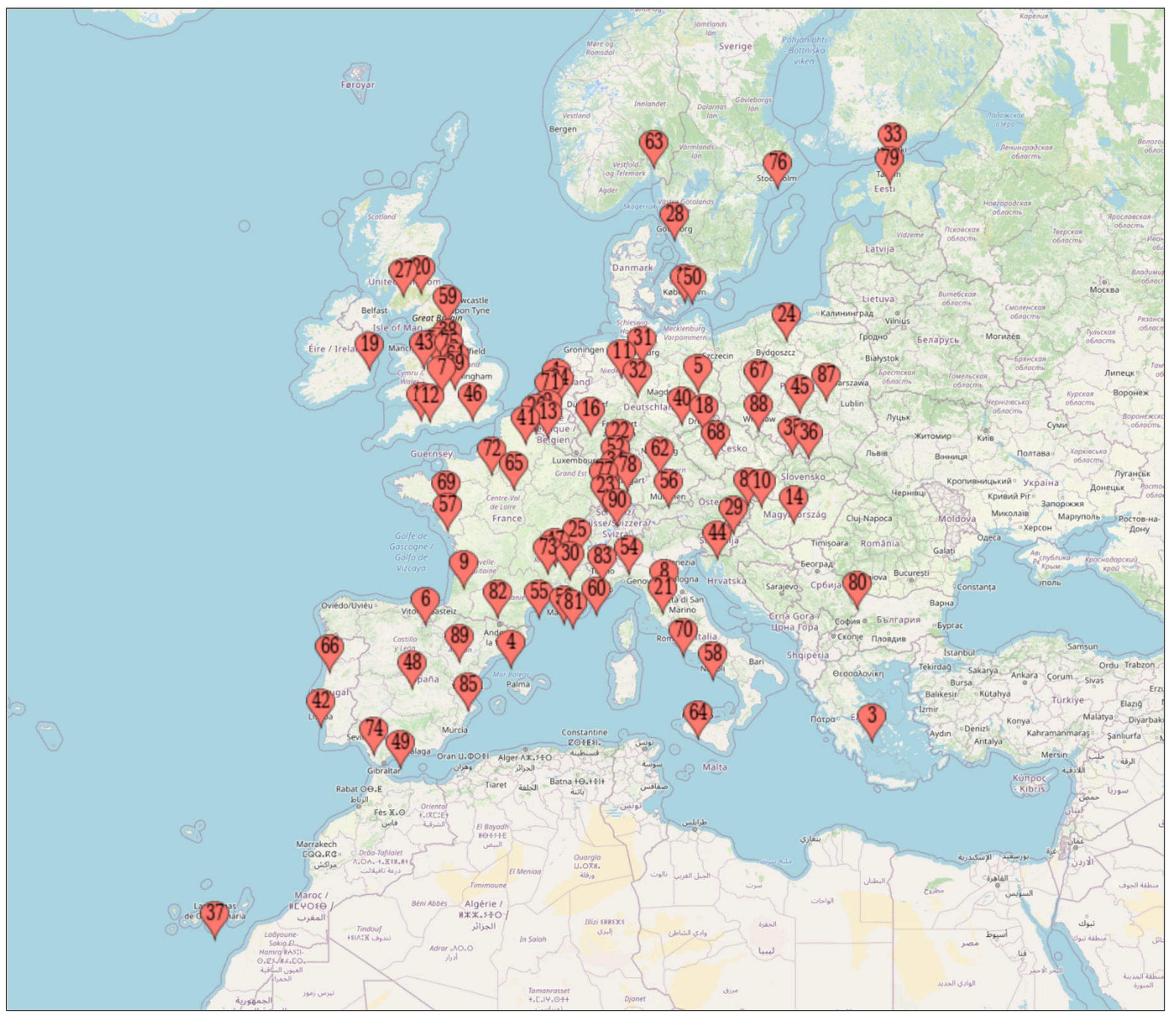
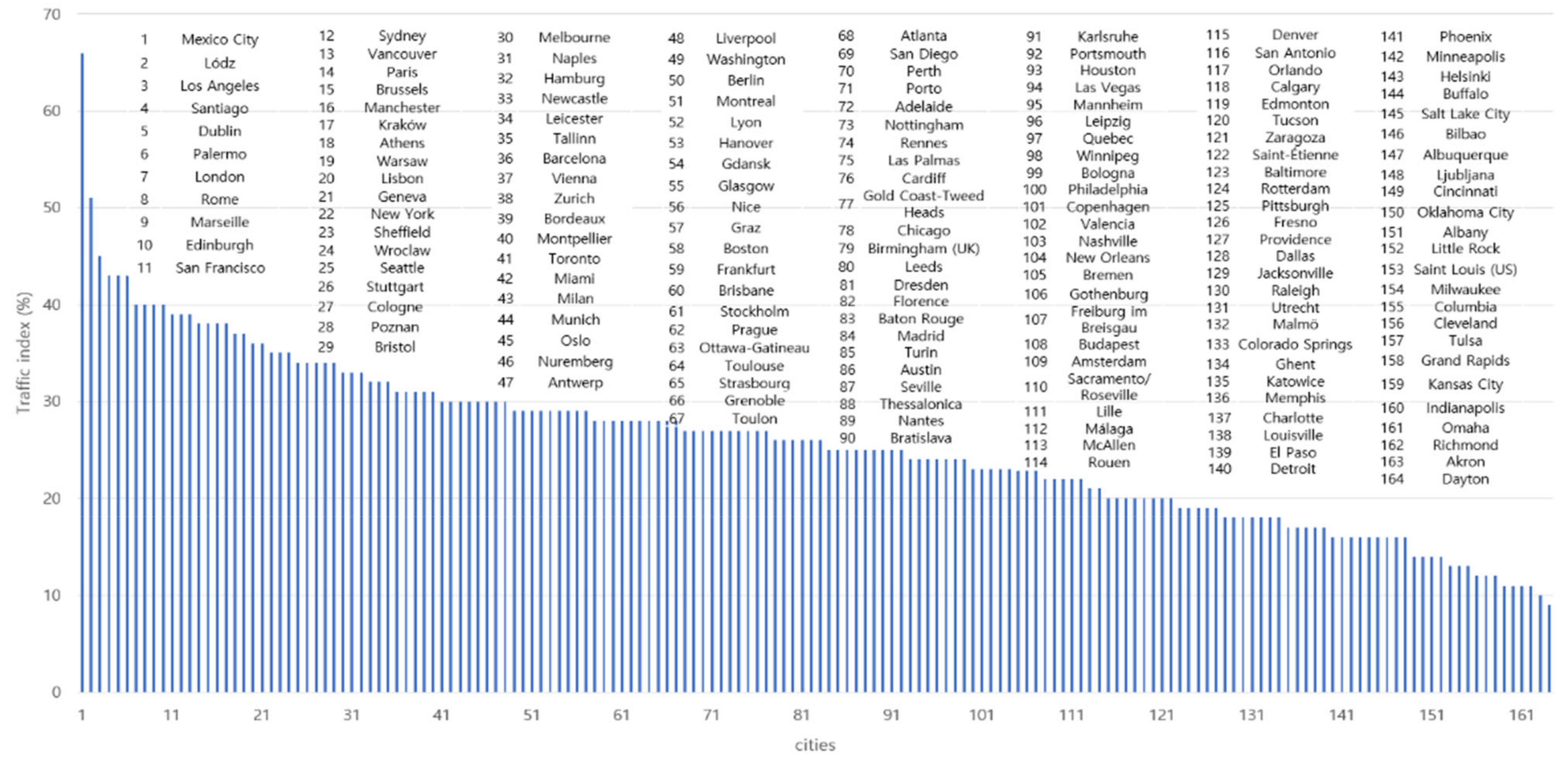
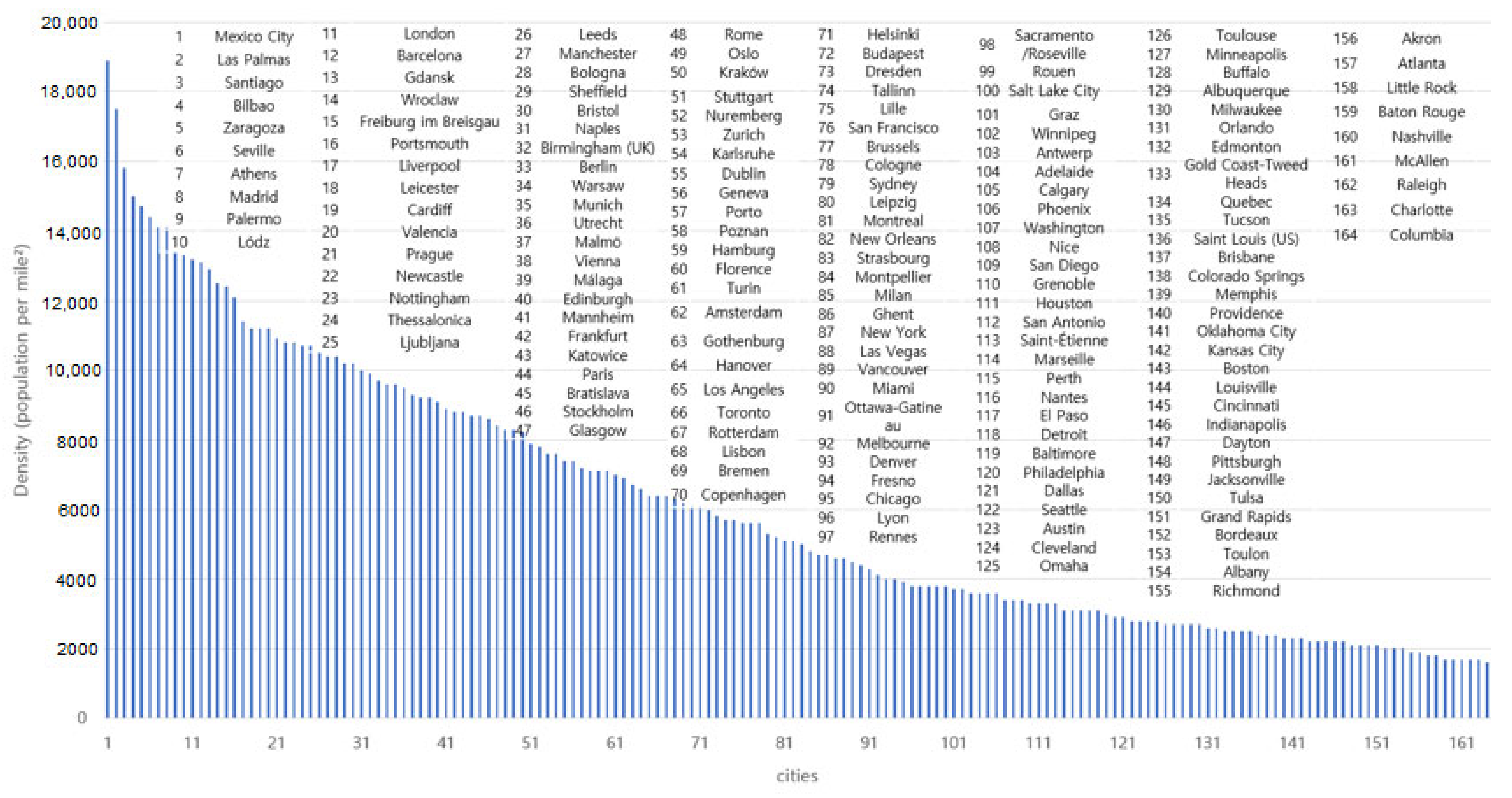
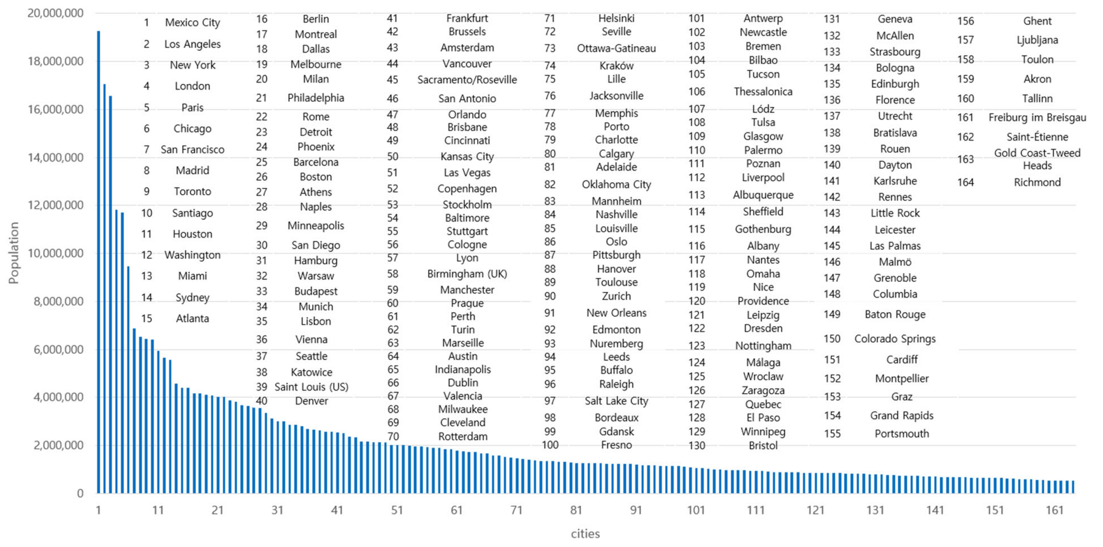
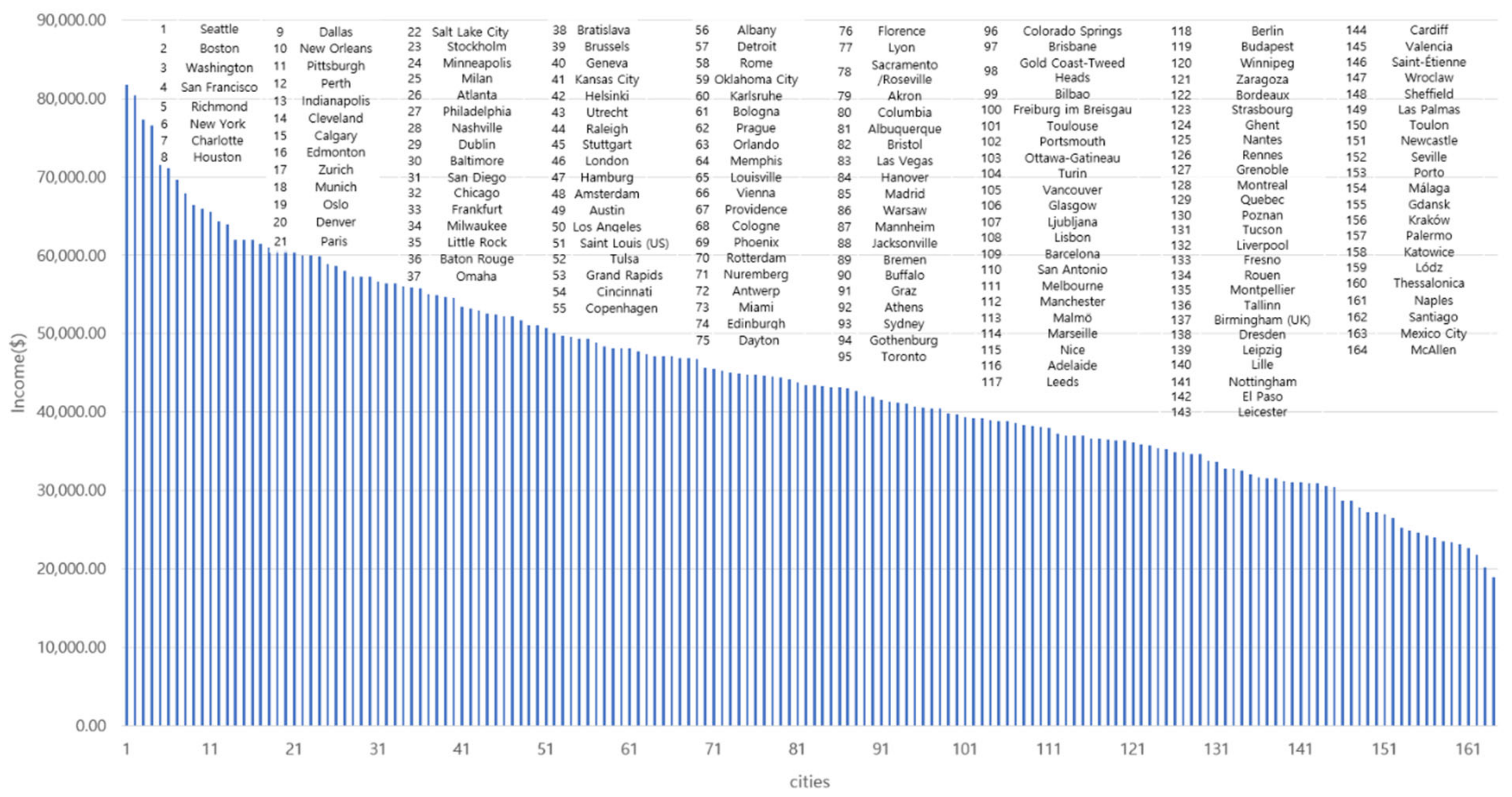
We were able to generate data for 164 cities with complete matching data sets of the traffic index, income per capita, population size, and population density for this analysis. Figure 2, Figure 3 and Figure 4 display 66 cities in the U.S. and 90 cities in Europe and 8 cities in Australia and Mexico respectively. The location of each city in the map is identified in number. Furthermore, each city has its traffic index listed. For example, Akron in the U.S. is numbered as ① in the map and has its traffic index ranked as T163 among the 164 cities. In addition, Figure 5, Figure 6, Figure 7 and Figure 8 provide rank distribution of 164 countries in traffic index, density, population and income per capita.
The 164 cities were then further divided into two groups: (1) 66 U.S.-Canadian cities and (2) 98 cities in 14 mostly European countries including Germany, United Kingdom, France, Spain, Poland, Australia, Italy, Netherlands, Belgium, Norway, Switzerland, Ireland, and Mexico. The population density of 66 cities was estimated at 3139 persons per square mile, while the density of 98 cities was higher at 8169 persons, as shown in Appendix A Table A1.
The averaged traffic index for the 98 cities was again higher at 29.3 over 20.5 for the 66 cities. As for income per capita, the average for the 66 cities was higher at $52,048 over $39,636 for the 98 cities. Finally, the averaged population size for the 66 cities was again higher at 2.598 million over 1.994 million for the 98 cities.

4. Analysis of Results

The correlation analysis of both dependent variable (traffic index) and three independent variables (population, income, and density) is shown in Table 2. The results indicated that statistically significant correlation between population size and population density did not exist.
The results of the multivariate regression of the STIRPAT model on traffic congestion index shown in Table 3 indicate that all three variables generated statistically significant coefficients at less than 1% level for the aggregate group of 164 cities with a density coefficient of 0.242, a population coefficient of 0.155, and an income coefficient of −0.20. These coefficients indicate that a 1% increase in population density is expected to increase traffic congestion by 0.242%, while the effects from population and income are held constant for the 164 cities. A 1% increase in population is expected to increase traffic congestion by 0.155%. In other words, the impact from density is greater than the impact from population size for the 164 cities. However, a 1% increase in income is expected to reduce traffic congestion by −0.2%, holding the effects from population and density constant.
The results of the same multivariate regression of the STIRPAT model on traffic congestion for the two disaggregate subgroups displayed a substantial difference. For the 98 high density cities primarily from Europe, only the population coefficient met less than the 1% level of statistical test of significance at 0.155 which was identical to the population coefficient of whole 164 cities at 0.155. The density coefficient displayed a marginal value of −0.004, while the income coefficient was −0.137.
In contrast, the 66 low density cities in the US-Canada had both density and population coefficients meeting the statistical test of significance at less than the 1% level, while their income coefficient failed to meet the statistical test of significance. In fact, the impact of density and population became greater at 0.311 and 0.207 respectively, compared to the coefficients for whole 164 cities. On the other hand, the income coefficients realized a negative value of −0.140 while feeling to meet the statistical test of significance.
In short, the results from the aggregate group of 164 cities and the first disaggregate group of low density 66 cities indicated that density was the key determinant whereas the second disaggregate group of high density 98 cities indicated that population was the exclusive determinant for traffic congestion, as shown in Figure 9.
In order to pursue now the question of urban scaling of traffic congestion [18,19,20,21,22,27], population size of cities for whole 164 cities were analyzed by the use of threshold panel regression [54]. The results as shown in Table 4 indicate that the optimal number of threshold was just one with the threshold value of ln14.675 or the population size of 2.138 million inhabitants. In other words, the aggregate group of 164 cities was divided into Region 1 or 46 cities with more than 2.138 million population and Region 2 of 113 cities with less than 2.138 million population.
All three independent variables generated statistically significant coefficients at less than the 1% level for the income and density coefficients and less than 5% level for the population coefficient from the Region 1. However, only the density and population coefficients from the Region 2 met the statistical test of significance at less than the 1% level.
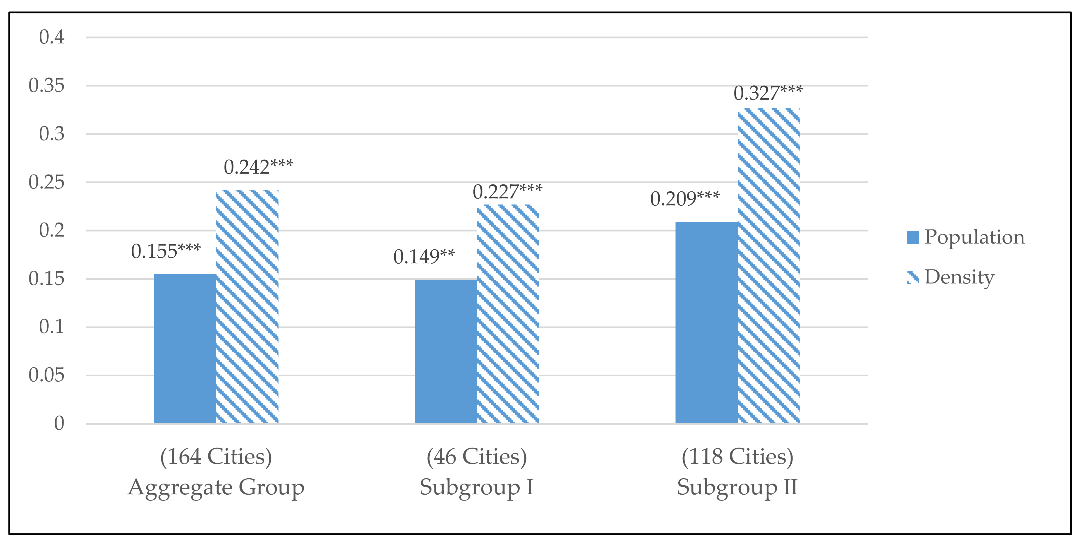
Comparing the population coefficient for the 46 large population cities at 0.149 to that of 118 smaller population cities at 0.209 supported a moderate scale advantage for the subgroup of large population size cities. To explain, a 1% increase of population size in the larger population city subgroup (Region 1) generated only 0.149% increase of traffic congestion, while a 1% increase of population size in the smaller population size subgroup would generate 0.209%, supporting the urban scale advantage in traffic congestion, as shown on Figure 10.
It is interesting to note that the density coefficient also displayed urban scale advantage in that a 1% increase in density generated smaller increase of congestion at 0.277% in the large population city subgroup overcome small population city subgroup at 0.327%. The same urban scaling advantage did exist on income in that a 1% increase in income generated a larger reduction of congestion at 0.349% in the large population city subgroup over −0.2% for the aggregate group of 164 cities. Finally, between density and population, density played somewhat greater impact to traffic congestion in large population subgroup as well as in small population subgroup, supporting the earlier finding from the whole 164 cities.

5. Conclusions

The key findings of this research can be summarized as follows. First, the results of multivariate regression on traffic congestion using the STIRPAT model for the aggregate group of 164 cities from 16 countries generated the most influential factor to be density with its coefficient at 0.242 over the population coefficient at 0.156. On the other hand, the income coefficient at −0.20 reduced congestion as income per capita in cities increased. All three coefficients met the statistical test of significance.
Second, the results from the same STIRPAT analysis for the disaggregate group of 66 low-density US-Canadian cities supported the results from the aggregate group with even higher density coefficient at 0.311 and a population coefficient at 0.207, both meeting the statistical test of significance. However, the income coefficient with a value of −0.140 failed to meet the statistical test of significance.
Third, the results of traffic congestion from the other disaggregate group of 98 high-density cities primarily from Europe generated that population coefficient at 0.155 was the only influential factor for traffic congestion. The density and income coefficients failed to meet the statistical test of significance. Besides, the density coefficient carried a very low value of 0.004.
Fourth, the use of threshold panel regression enabled the division of whole 164 cities into two regional subgroups of 46 larger population cities and the remaining 118 smaller population cities. Comparing the population coefficients between the subgroup of 46 larger population size cites and the subgroup of 118 smaller population-size cities, the same 1% increase in population resulted in 0.149% and 0.209% increase of traffic congestion respectively. Put it another way, the larger city would generate about 35% less traffic congestion from the same 1% increase of population size, compared to the smaller city.
Fifth, as for the difference of impact among the three variables, the large population subgroup of 46 cities displayed the order of impact from income at −0.349, followed by density at +0.227 and population at 0.149. The smaller population subgroup of 118 cities displayed the order of impact from density at +0.327 followed by population at +0.209.
In short, combining the use of STIRPAT model and threshold panel regression, we have analyzed traffic congestion in the aggregate group of 164 cities together with four disaggregate groups of 66 low-density cities, 98 high-density cities, 46 large population cities and 118 small population cities. Among the three independent variables of density, population, and income, statistically significant impact exercised by income was limited only in the two case of the aggregate group and the disaggregate group of large population cities. Therefore, focusing on the relative impact between remaining variables of density and population, population exercised the primary impact to congestion only in one case of the 98 high-density cities. In the remaining four cases, density has exercised greater impact over population to determine the level of traffic congestion.
These findings from the aggregate group indicate that traffic congestion in cities is influenced by varying density and population sizes. The findings from the disaggregate samples highlighted a clear difference in the critical role of density in low-density cities and the exclusive role of population size in high-density cities. Further threshold analysis by population-based subgroups in the aggregate group established the existence of both a population and density scale advantage to traffic congestion.
This study has several implications for researchers and city planners. For evaluation and planning of traffic congestion, individual cities may want to begin their analysis with an aggregate sample of cities and use all three determinants of density, population, and income since this research established statistically significant coefficients for all three factors. Next, if a disaggregate analysis between cities with low versus high density is possible, then a high-density city may wish to focus on analyzing a disaggregate group of high-density cities and use population and other determinants, because an additional increase of density in highly compact cities may have little impact on traffic congestion as suggested by Kenworthy and Laube [8] and many others. In contrast, the population scale advantage of congestion indicates that cities with a larger population may experience proportionately less congestion.
A low-density city, however, may wish to focus on a disaggregate group of low-density cities and use density as the primary determinant together with population and other variables. This research estimated that the size of the density coefficient was nearly 82 percent larger than the population coefficient from the 64 low-density cities (0.351/0.193). However, this study also indicates that using both density and population as determinants is preferred, as both variables met the statistical test of significance.
In summary, the use of aggregate analysis where high- and low-density cities are combined may generate both density and population coefficients, which may not always be appropriate to evaluate traffic congestion for individual cities with either low or high density. In other words, the results from an aggregate study with a large cross-country sample needs to be verified with appropriately designed disaggregate studies before developing specific policy implications for an individual city or country. Furthermore, empirical findings of population scale advantage on traffic congestion provide valuable supporting evidence to earlier studies of urban scaling of traffic congestion [21,22,27].
This study has several limitations that provide opportunities for future studies. Due to the unavailability of relevant data, this study was unable to account for several other possible determining factors for traffic congestion. These other factors may include automobile density, percent of the commuting population, traffic control systems, traffic regulations, road conditions, weather, and many other factors that vary across cities in multiple countries. The use of the TomTom traffic index may be another limitation in that the index cannot be verified by other data sources.
Despite these limitations, this research has established the role of both population density and population size of cities as important determining factors in traffic congestion. Equally important is that it is essential to use disaggregate samples based on density and/or population in future studies of traffic congestion.

Author Contributions

Formal analysis, Y.-T.L. and Y.L.; methodology, Y.S.C.; writing—original draft, Y.S.C. and S.J.J.; writing—review and editing, S.J.J. and Y.L. All authors have read and agreed to the published version of the manuscript.

Funding

This research received no external funding.

Institutional Review Board Statement

Not applicable.

Informed Consent Statement

Not applicable.

Data Availability Statement

Data sources are reported in our Method and Data section. Data are available from these sources.

Acknowledgments

The authors are very grateful for an anonymous reviewer, who suggested many ideas to improve the quality of the paper. Competent and sincere help provided by research assistants, Su Min Kim and Young Eun Kim, at the Gachon Center for Convergence Research is also appreciated.

Conflicts of Interest

The authors declare no conflict of interest.

Appendix A

Table A1. Traffic Index, Population, Income and Density for the Total Group of 164 Cities.
Rank of PopulationCityTraffic Index (%)Population (2010)Income per Capita (in $)Density (Population per m2)
1Mexico City6619,255,92120,215.6318,900
2Los Angeles4517,053,74551,053.366400
3New York3516,539,42971,109.834600
4London4011,793,53052,237.9513,200
5Paris3811,693,21960,450.158700
6Chicago269,461,10456,441.723900
7San Francisco396,848,02876,564.965600
8Madrid256,507,50243,229.8414,100
9Toronto306,418,62340,672.786400
10Santiago436,393,83021,815.3115,800
11Houston245,920,50067,964.363300
12Washington295,636,18577,356.43400
13Miami305,564,64145,055.924400
14Sydney394,555,51641,163.055300
15Atlanta274,377,19758,611.711800
16Berlin294,374,70836,532.489700
17Montreal294,169,71434,588.15100
18Dallas184,145,12466,430.822900
19Melbourne334,105,85837,940.974100
20Milan304,060,62458,845.94700
21Philadelphia234,024,83058,040.462900
22Rome404,008,09548,383.298300
23Detroit163,863,92448,862.763100
24Phoenix163,817,11746,708.033600
25Barcelona313,675,20638,232.7913,100
26Boston283,639,14480,446.392200
27Athens373,563,60741,327.1914,100
28Naples333,552,56822,693.6110,000
29Minneapolis163,348,85959,931.462700
30San Diego273,095,31356,602.033400
31Hamburg332,984,96652,203.597100
32Warsaw372,981,19843,220.629600
33Budapest222,846,46436,383.26000
34Munich302,844,74960,969.989600
35Lisbon362,797,61238,308.216300
36Vienna312,683,25147,076.799200
37Seattle342,644,46681,820.32800
38Katowice172,628,20723,544.088800
39Saint Louis (US)132,559,92650,708.892500
40Denver202,551,34160,606.954000
41Frankfurt282,517,80556,430.538800
42Brussels382,485,48054,631.335600
43Amsterdam222,360,95851,664.76900
44Vancouver392,312,49738,896.624500
45Sacramento/Roseville222,149,12744,583.683800
46San Antonio202,142,50838,053.073300
47Orlando202,134,41147,411.672600
48Brisbane282,108,34840,495.972400
49Cincinnati142,107,07449,612.882200
50Kansas City112,009,34453,458.742300
51Las Vegas241,995,21543,392.824600
52Copenhagen231,989,87149,396.26100
53Stockholm281,964,82959,970.738600
54Baltimore191,957,90157,239.363000
55Stuttgart341,954,75652,425.897900
56Cologne341,903,15446,880.745600
57Lyon291,894,94544,700.193800
58Birmingham (UK)261,884,19931,555.119900
59Manchester381,841,38237,290.1810,400
60Prague281,829,84347,763.910,900
61Perth271,781,13264,368.883100
62Turin251,747,61439,0197000
63Marseille401,722,23637,015.143100
64Austin251,716,28351,069.082800
65Indianapolis111,658,60063,942.482200
66Dublin431,650,20257,273.717400
67Valencia231,570,51730,441.5511,200
68Milwaukee131,555,90856,077.222700
69Cleveland121,510,16362,025.092800
70Rotterdam191,484,83045,676.026400
71Helsinki161,455,67753,154.436100
72Seville251,421,04526,445.1614,400
73Ottawa-Gatineau281,386,54439,189.634300
74Kraków381,351,83124,237.58200
75Lille221,349,19431,022.565700
76Jacksonville181,345,59642,674.772100
77Memphis171,324,82947,111.742400
78Porto271,300,28525,300.077200
79Charlotte171,298,93169,592.611700
80Calgary201,271,73761,957.943600
81Adelaide271,253,09736,662.653600
82Oklahoma City141,252,98748,159.322300
83Mannheim241,240,96442,997.928900
84Nashville231,239,56557,311.231700
85Louisville171,235,70847,104.172200
86Oslo301,225,20260,611.418300
87Pittsburgh191,223,42365,591.382100
88Hanover291,222,77343,258.586600
89Toulouse281,217,31639,352.552700
90Zurich311,206,31261,496.197600
91New Orleans231,189,86665,883.895100
92Edmonton201,169,70161,957.942600
93Nuremberg301,166,97645,539.947800
94Leeds261,166,26736,564.4810,500
95Buffalo161,135,50941,937.142700
96Raleigh181,130,64152,516.231700
97Salt Lake City161,125,30159,997.283800
98Bordeaux311,121,98335,859.62000
99Gdansk291,091,85024,647.3712,900
100Fresno191,081,74232,741.634000
101Antwerp301,053,72545,242.083600
102Newcastle321,050,56126,967.7410,800
103Bremen231,025,58042,069.646200
104Bilbao16997,31139,892.9615,000
105Tucson20980,26333,647.092500
106Thessalonica25957,94623,153.7310,700
107Lódz51956,15623,413.2213,300
108Tulsa12948,01450,150.12100
109Glasgow29947,80838,793.748400
110Palermo43935,92123,983.3813,400
111Poznan34934,00133,721.757100
112Liverpool30929,01432,751.6911,400
113Albuquerque16887,07743,740.282700
114Sheffield35880,23627,884.310,200
115Gothenburg23877,14941,114.966700
116Albany14870,71049,349.382000
117Nantes25870,04535,281.283100
118Omaha11865,35055,089.852800
119Nice29845,18636,935.753400
120Providence19842,70046,882.642300
121Leipzig24837,61031,192.135200
122Dresden26836,99531,540.95800
123Nottingham27835,62531,018.810,800
124Málaga22834,02324,858.779200
125Wroclaw35832,97428,682.2812,500
126Zaragoza20825,83736,155.3414,700
127Quebec24820,52934,588.12500
128El Paso17804,12230,984.073100
129Winnipeg24803,60136,342.143700
130Bristol34795,48043,403.1410,200
131Geneva36785,02254,529.927400
132McAllen21774,76818,937.261700
133Strasbourg28758,72435,761.875000
134Bologna24745,25448,110.4310,400
135Edinburgh40727,61944,885.339100
136Florence26723,16444,815.397100
137Utrecht18716,64852,927.469500
138Bratislava25715,45554,881.978700
139Rouen21698,38532,486.723800
140Dayton9696,72644,823.932200
141Karlsruhe25686,93848,127.257600
142Rennes27671,92934,897.793800
143Little Rock14671,45955,966.191800
144Leicester32660,81730,950.1411,200
145Las Palmas27658,95727,249.8917,500
146Malmö18656,83437,027.869300
147Grenoble28649,28534,839.833300
148Columbia13646,87744,153.681600
149Baton Rouge26645,63955,743.221700
150Colorado Springs18645,62640,548.242400
151Cardiff27640,63230,532.1311,200
152Montpellier31635,89732,078.64800
153Graz29608,42041,510.683700
154Grand Rapids12602,62249,789.092100
155Portsmouth25577,19139,255.5712,100
156Ghent18576,40835,359.674700
157Ljubljana16567,09738,662.3710,700
158Toulon28547,70227,216.782000
159Akron10541,78144,418.321900
160Tallinn32530,76031,661.925700
161Freiburg im Breisgau23527,58139,673.212,400
162Saint-Étienne20520,66728,743.963300
163Gold Coast-Tweed Heads27519,63040,495.972500
164Richmond11511,14971,732.511900
Average164 Cities
(Total)
25.82,236,92144,631.826145
66 Cities
(U.S.-Canada)
20.52,598,12952,048.613139
98 Cities
(Remaining countries)
29.31,993,65839,636.838169

References

  1. Zhang, K.; Batterman, S. Air pollution and health risks due to vehicle traffic. Sci. Total Environ. 2013, 450, 307–316. [Google Scholar] [CrossRef] [PubMed] [Green Version]
  2. Levy, J.I.; Buonocore, J.J.; Von Stackelberg, K. Evaluation of the public health impacts of traffic congestion: A health risk assessment. Environ. Health A Glob. Access Sci. Source 2010, 9, 65. [Google Scholar] [CrossRef] [Green Version]
  3. Sweet, M. Does traffic congestion slow the economy? J. Plan. Lit. 2011, 26, 391–404. [Google Scholar] [CrossRef]
  4. Weisbrod, G.; Vary, D.; Treyz, G. Measuring economic costs of urban traffic congestion to business. Transp. Res. Rec. 2003, 1839, 98–106. [Google Scholar] [CrossRef] [Green Version]
  5. Ewing, R.; Cervero, R. Travel and the built environment: A meta-analysis. J. Am. Plan. Assoc. 2010, 76, 265–294. [Google Scholar] [CrossRef]
  6. Stevens, M.R. Does compact development make people drive less? J. Am. Plan. Assoc. 2017, 83, 7–18. [Google Scholar] [CrossRef]
  7. Newman, P.; Kenworthy, J. Cities and Automobile Dependence: An International Sourcebook; Gower Technical: Aldershot, UK, 1989. [Google Scholar]
  8. Kenworthy, J.R.; Laube, F.B. Patterns of automobile dependence in cities: An international overview of key physical and economic dimensions with some implica tions for urban policy. Transp. Res. Part A Policy Pract. 1999, 33, 691–723. [Google Scholar] [CrossRef]
  9. TomTom Traffic Index. 2016. Available online: https://www.tomtom.com/en_gb/trafficindex. (accessed on 20 December 2020).
  10. Cohn, N. Real-time traffic information and navigation: An operational system. Trans. Res. Rec. 2009, 2129, 129–135. [Google Scholar] [CrossRef]
  11. Boarnet, M.G. A broader context for land use and travel behavior, and a research agenda. J. Am. Plan. Assoc. 2011, 77, 197–213. [Google Scholar] [CrossRef]
  12. Karathodorou, N.; Graham, D.J.; Noland, R.B. Estimating the effect of urban density on fuel demand. Energy Econ. 2010, 32, 86–92. [Google Scholar] [CrossRef] [Green Version]
  13. Sue, Q. The effect of population density, road network density, and congestion on household gasoline consumption in U.S. urban areas. Energy Econ. 2011, 33, 445–452. [Google Scholar] [CrossRef]
  14. Ye, H.; He, X.; Song, Y.; Li, X.; Zhang, G.; Lin, T.; Xiao, L. A sustainable urban form: The challenges of compactness from the viewpoint of energy consumption and carbon emission. Energy Build. 2015, 93, 90–98. [Google Scholar] [CrossRef]
  15. Gudipudi, R.; Fluschnik, T.; Ros, A.G.C.; Walther, C.; Kropp, J.P. City density and CO2 efficiency. Energy Policy 2016, 91, 352–361. [Google Scholar] [CrossRef]
  16. Bettencourt, L.M.A.; Lobo, J.; Helbing, D.; Kühnert, C.; West, G.B. Growth, innovation, scaling, and the pace of life in cities. Proc. Natl. Acad. Sci. USA 2007, 104, 7301–7306. [Google Scholar] [CrossRef] [PubMed] [Green Version]
  17. Bettencourt, L.M.A.; Lobo, J.; Strumsky, D.; West, G.B. Urban scaling and its deviations: Revealing the structure of wealth, innovation and crime across cities. PLoS ONE 2010, 5, e13541. [Google Scholar] [CrossRef] [Green Version]
  18. Fragkias, M.; Lobo, J.; Strumsky, D.; Seto, K.C. Does size matter? Scaling of CO2 emissions and U.S. Urban areas. PLoS ONE 2013, 8, e64727. [Google Scholar] [CrossRef]
  19. Oliveira, E.A.; Andrade, J.S.; Makse, H.A. Large cities are less green. Sci. Rep. 2014, 4, 4235. [Google Scholar] [CrossRef] [PubMed] [Green Version]
  20. Muller, N.Z.; Jha, A. Does environmental policy affect scaling laws between population and pollution? Evidence from American metropolitan areas. PLoS ONE 2017, 12, e0181407. [Google Scholar]
  21. Louf, R.; Barthelemy, M. How congestion shapes cities: From mobility patterns to scaling. Sci. Rep. 2014, 4, 5561. [Google Scholar] [CrossRef] [PubMed]
  22. Barthelemy, M. A global take on congestion in urban areas. Environ. Plan. B Plan. Des. 2016, 43, 800–804. [Google Scholar] [CrossRef] [Green Version]
  23. Bento, A.M.; Cropper, M.L.; Mobarak, A.M.; Vinha, K. The effects of urban spatial structure on travel demand in the United States. Rev. Econ. Stat. 2005, 87, 466–478. [Google Scholar] [CrossRef]
  24. Bhat, C.R.; Guo, J.Y. A comprehensive analysis of built environment characteristics on household residential choice and auto ownership levels. Transp. Res. Part B Methodol. 2007, 41, 506–526. [Google Scholar] [CrossRef] [Green Version]
  25. Brownstone, D.; Golob, T.F. The impact of residential density on vehicle usage and energy consumption. J. Urban Econ. 2009, 65, 91–98. [Google Scholar] [CrossRef] [Green Version]
  26. Duranton, G.; Turner, M.A. Urban form and driving: Evidence from US cities. J. Urban Econ. 2018, 108, 170–191. [Google Scholar] [CrossRef]
  27. Chang, Y.S.; Lee, Y.J.; Choi, S.S. Is there more traffic congestion in larger cities? Scaling analysis of the 101 largest U.S. urban centers. Trans. Policy 2017, 59, 54–63. [Google Scholar] [CrossRef]
  28. Lu, J.; Li, B.; Li, H.; Al-Barakani, A. Expansion of city scale, traffic modes, traffic congestion, and air pollution. Cities 2021, 108, 102974. [Google Scholar] [CrossRef]
  29. Ribeiro, H.V.; Rybski, D.; Kropp, J.P. Effects of changing population or density on urban carbon dioxide emissions. Nat. Commun. 2019, 10, 3204. [Google Scholar] [CrossRef] [Green Version]
  30. Bertaud, A.; Richardson, H.W. Transit and density: Atlanta, the United States and western Europe. In Urban Sprawl in Western Europe and the United States; Richardson, A., Bae, C., Eds.; Ashgate: London, UK, 2004; pp. 293–310. [Google Scholar]
  31. Freemark, Y. Is Transit Ridership Loss Inevitable? A U.S.-France Comparison. Available online: https://www.thetransportpolitic.com/2019/09/09/is-transit-ridership-loss-inevitable-a-u-s-france-comparison/ (accessed on 6 April 2021).
  32. Transport Research Board. Making Transit Work: Insight from Western Europe, Canada, and the United States. Available online: https://www.nap.edu/catalog/10110/making-transit-work-insight-from-western-europe-canada-and-the (accessed on 6 April 2021).
  33. Dietz, T.; Rosa, E.A. Rethinking the environmental impacts of population, affluence and technology. Hum. Ecol. Rev. 1994, 1, 277–300. [Google Scholar]
  34. Holdren, J.P.; Ehrlich, P.R. Human population and the global environment: Population growth, rising per capita material consumption, and disruptive technologies have made civilization a global ecological force. Am. Sci. 1974, 62, 282–292. [Google Scholar] [PubMed]
  35. York, R.; Rosa, E.A.; Dietz, T. STIRPAT, IPAT and ImPACT: Analytic tools for unpacking the driving forces of environmental impacts. Ecol. Econ. 2003, 46, 351–365. [Google Scholar] [CrossRef]
  36. Shi, A. The impact of population pressure on global carbon dioxide emissions, 1975–1996: Evidence from pooled cross-country data. Ecol. Econ. 2003, 44, 29–42. [Google Scholar] [CrossRef]
  37. Cole, M.A.; Neumayer, E. Examining the impact of demographic factors on air pollution. Popul. Environ. 2004, 26, 5–21. [Google Scholar] [CrossRef] [Green Version]
  38. Martínez-Zarzoso, I.; Bengochea-Morancho, A.; Morales-Lage, R. The impact of population on CO2 emissions: Evidence from European countries. Environ. Resour. Econ. 2007, 38, 497–512. [Google Scholar] [CrossRef] [Green Version]
  39. Poumanyvong, P.; Kaneko, S. Does urbanization lead to less energy use and lower CO2 emissions? A cross-country analysis. Ecol. Econ. 2010, 70, 434–444. [Google Scholar] [CrossRef]
  40. Martínez-Zarzoso, I.; Maruotti, A. The impact of urbanization on CO2 emissions: Evidence from developing countries. Ecol. Econ. 2011, 70, 1344–1353. [Google Scholar] [CrossRef] [Green Version]
  41. Dietz, T.; Rosa, E.A.; York, R. Environmentally efficient weil-being: Rethinking sustainability as the relationship between human well-being and environmental impacts. Hum. Ecol. Rev. 2009, 16, 114–123. [Google Scholar]
  42. Steinberger, J.K.; Krausmann, F.; Eisenmenger, N. Global patterns of materials use: A socioeconomic and geophysical analysis. Ecol. Econ. 2010, 69, 1148–1158. [Google Scholar] [CrossRef]
  43. Fischer-Kowalski, M.; Krausmann, F.; Giljum, S.; Lutter, S.; Mayer, A.; Bringezu, S.; Weisz, H. Methodology and indicators of economy wide material flow accounting. J. Ind. Ecol. 2011, 15, 855–876. [Google Scholar] [CrossRef]
  44. Chertow, M.R. The IPAT Equation and Its Variants. J. Ind. Ecol. 2000, 25, 313–337. [Google Scholar] [CrossRef]
  45. Uddin, G.A.; Alam, K.; Gow, G. Estimating the Major Contributors to Environmental Impacts in Australia. Environ. Ecol. Stat. 2016, 37, 1–14. [Google Scholar]
  46. Wang, M.; Che, Y.; Yang, K.; Wang, M.; Xiong, L.; Huang, Y. A local-scale low-carbon plan based on the STIRPAT model and the scenario method: The case of Minhang District, Shanghai, China. Energy Policy 2011, 19, 6981–6990. [Google Scholar] [CrossRef]
  47. Hansen, B.E. Threshold effects in non-dynamic panels: Estimation, testing, and inference. J. Econ. 1999, 93, 345–368. [Google Scholar] [CrossRef] [Green Version]
  48. Qi, S.; Li, Y. Threshold effects of renewable energy consumption on economic growth under energy transformation. Chinese J. Popul. Resour. Environ. 2017, 15, 312–321. [Google Scholar] [CrossRef]
  49. Yi, S.; Xiao, L.A. Application of threshold regression analysis to study the impact of regional technological innovation level on sustainable development. Renew. Sust. Energ. Rev. 2018, 89, 27–32. [Google Scholar] [CrossRef]
  50. Wu, H.T.; Hao, Y.; Weng, J.H. How does energy consumption affect China’s urbanization? New evidence from dynamic threshold panel models. Energy Policy 2019, 127, 24–38. [Google Scholar] [CrossRef]
  51. Qi, J. Study on the threshold effect of China’s industrial structure on carbon emission. IOP Conf. Ser. Earth Environ. Sci. 2020, 546, 022053. [Google Scholar] [CrossRef]
  52. Han, D.; Li, T.; Feng, S.; Shi, Z. Application of Threshold Regression Analysis to Study the Impact of Clean Energy Development on China’s Carbon Productivity. Int. J. Environ. Res. Public Health 2020, 17, 1060. [Google Scholar] [CrossRef] [Green Version]
  53. Raza, S.A.; Shah, N.; Qureshi, M.A.; Qaiser, S.; Ali, R.; Ahmed, F. Non-linear threshold effect of financial development on renewable energy consumption: Evidence from panel smooth trnsition regression approach. Environ. Sci. Pollut. Res. 2020, 27, 32034–32047. [Google Scholar] [CrossRef]
  54. Chang, T.H.; Huang, C.M.; Lee, M.C. Threshold effect of the economic growth rate on the renewable energy development from a change in energy price: Evidence from OECD countries. Energy Policy 2009, 37, 5796–5802. [Google Scholar] [CrossRef]
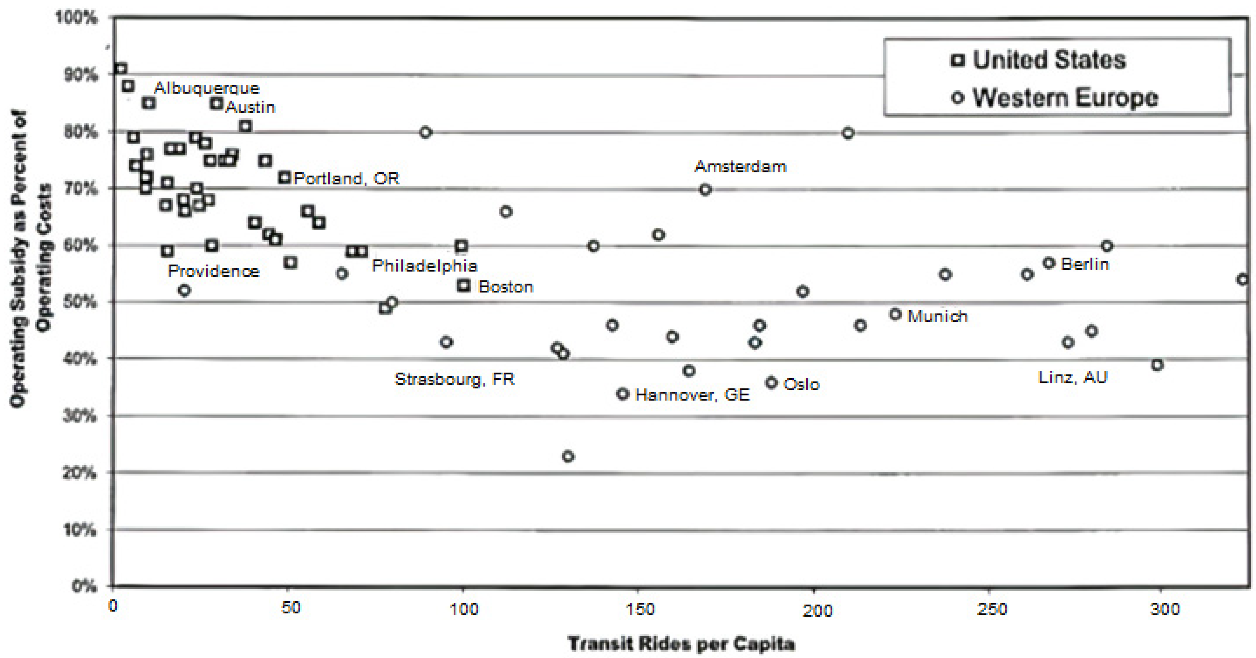
Figure 1. Public operating subsidies and transit ridership levels for selected US and Western European urban areas.
Sustainability 13 04280 g001
Figure 2. 66 Cities in the U.S. and Canada. 1. Akron(163) 2. Albany(T149) 3. Albuquerque(T140) 4. Atlanta(T68) 5. Austin(T84) 6. Baltimore(T123) 7. Baton Rouge(T78) 8. Boston(T58) 9. Buffalo(T140) 10. Calgary(T115) 11. Charlotte(T135) 12. Chicago(T78) 13. Cincinnati(T149) 14. Cleveland(T156) 15. Colorado Springs(T128) 16. Columbia(T153) 17. Dallas(T128) 18. Dayton(164) 19. Denver(T115) 20. Detroit(T140) 21. Edmonton(T115) 22. El Paso(T135) 23. Fresno(T123) 24. Grand Rapids(T156) 25. Houston(T93) 26. Indianapolis(T159) 27. Jacksonville(T128) 28. Kansas City(T159) 29. Las Vegas(T93) 30. Little Rock(T149) 31. Los Angeles(3) 32. Louisville(T135) 33. McAllen(T113) 34. Memphis(T135) 35. Miami(T41) 36. Milwaukee(T153) 37. Minneapolis(T140) 38. Montreal(T49) 39. Nashville(T100) 40. New Orleans(T100) 41. New York(T22) 42. Oklahoma City(T149) 43. Omaha(T159) 44. Orlando(T115) 45. Ottawa(T58) 46. Philadelphia(T100) 47. Phoenix(T140) 48. Pittsburgh(T123) 49. Portsmouth(T84) 50. Providence(T123) 51. Quebec(T93) 52. Raleigh(T128) 53. Richmond(T159) 54. Sacramento(T108) 55. Salt Lake City(T140) 56. San Antonio(T115) 57. San Diego(T68) 58. San Francisco(T11) 59. Seattle(T25) 60. St. Louis(T153) 61. Toronto(T41) 62. Tucson(T115) 63. Tulsa(T156) 64. Vancouver(T11) 65. Washington(T49) 66. Winnipeg(T93).
Sustainability 13 04280 g002
Figure 3. 90 Cities in Europe. 1. Amsterdam(T108) 2. Antwerp(T41) 3. Athens(T18) 4. Barcelona(T36) 5. Berlin(T49) 6. Bilbao(T140) 7. Birmingham(T78) 8. Bologna(T93) 9. Bordeaux(T36) 10. Bratislava(T84) 11. Bremen(T100) 12. Bristol(T25) 13. Brussels(T14) 14. Budapest(T108) 15. Cardiff(T68) 16. Cologne(T25) 17. Copenhagen(T100) 18. Dresden(T78) 19. Dublin(T4) 20. Edinburgh(T7) 21. Florence(T78) 22. Frankfurt(T58) 23. Freiburg(T100) 24. Gdansk(T49) 25. Geneva(T20) 26. Ghent(T128) 27. Glasgow(T49) 28. Gothenburg(T100) 29. Graz(T49) 30. Grenoble(T58) 31. Hamburg(T30) 32. Hanover(T49) 33. Helsinki(T140) 34. Karlsuhe(T84) 35. Katowice(T135) 36. Krakow(T14) 37. Las Palmas(T68) 38. Leeds(T78) 39. Leicester(T33) 40. Leipzig(T93) 41. Lille(T108) 42. Lisbon(T20) 43. Liverpool(T41) 44. Ljublijana(T140) 45. Lodz(2) 46. London(T7) 47. Lyon(T49) 48. Madrid(T84) 49. Malaga(T108) 50. Malmo(T128) 51. Manchester(T14) 52. Mannheim(T93) 53. Marseille(T7) 54. Milan(T41) 55. Montpellier(T36) 56. Munich(T41) 57. Nantes(T84) 58. Naples(T30) 59. Newcastle(T33) 60. Nice(T49) 61. Nottingham(T68) 62. Nuremberg(T41) 63. Oslo(T41) 64. Palermo(T4) 65. Paris(T14) 66. Porto(T68) 67. Poznan(T25) 68. Prague(T58) 69. Rennes(T68) 70. Rome(T7) 71. Rotterdam(T123) 72. Rouen(T113) 73. Saint-Etienne(T115) 74. Seville(84) 75. Sheffield(T22) 76. Stockholm(T58) 77. Strasbourg(T58) 78. Stuttgart(T25) 79. Tallinn(T33) 80. Thessalonica(T84) 81. Toulon(T58) 82. Toulouse(T58) 83. Turin(T84) 84. Utrecht(T128) 85. Valencia(T100) 86. Vienna(T36) 87. Warsaw(T18) 88. Wroclaw(T22) 89. Zaragoza(T115) 90. Zurich(T36).
Sustainability 13 04280 g003
Figure 4. 8 Cities in Central America, South America, and Australia. 1. Adelaide(T68) 2. Brisbane(T58) 3. Gold Coast(T68) 4. Melbourne(T30) 5. Mexico City(1) 6. Perth(T68) 7. Santiago(T4) 8. Sydney(T11).
Sustainability 13 04280 g004
Figure 5. Rank Distribution of Traffic Index.
Sustainability 13 04280 g005
Figure 6. Rank Distribution of Density.
Sustainability 13 04280 g006
Figure 7. Rank Distribution of Population.
Sustainability 13 04280 g007
Figure 8. Rank Distribution of Income.
Sustainability 13 04280 g008
Figure 9. Density and Population Coefficient from Multivariate Regression from an Aggregate Group of 164 Cities, and Disaggregate Groups of 98 Cities and 66 Cities. *** Significant at 1% level.
Sustainability 13 04280 g009
Figure 10. Density and Population Coefficient from Threshold Multivariate Regression for Aggregate Group of 164 Cities, and Population Subgroups of 118 Cities and 46 Cities. *** Significant at 1% level. ** Significant at 5% level.
Sustainability 13 04280 g010
Table 1. Comparing transit capacity and usage between the European and the U.S. cities (1990).
CitiesTransit Service km per PersonRail Service Intensity (Service km per Urban ha)Percentage of Total Motorized Passenger km on TransitPercentage of Workers Using Transit
European (11)92 km3651 km22.6%38.8%
American (13)28 km153 km3.1%9.0%
European American 3.28 times23.86 times7.29 times4.31 times
Source: Kenworthy and Laube [8].
Table 2. Correlations among Variables.
In_Traffic IndexIn_DensityIn_PopulationIn_Income
In_Traffic Index 1.000 - - -
In_Density0.556 **1.000--
In_Population0.351 **0.1231.000-
In_Income−0.257 **−0.409 **0.27 **1.000
** Correlation is significant at the 0.05 level (2-tailed).
Table 3. Multivariate Regression of Traffic Index by Aggregate Group of 164 Cities, Disaggregate Groups of 98 Cities and 66 Cities.
Variable\Group Aggregate Group
(164 Cities)
Disaggregate Group 1
(66 Cities)
Disaggregate Group 2
(98 Cities)
ln_Density0.242 ***
(0.039)
0.311 ***
(0.077)
−0.004
(0.042)
ln_Population0.155 ***
(0.027)
0.207 ***
(0.039)
0.155 ***
(0.035)
ln_Income−0.200 **
(0.083)
−0.140
(0.142)
−0.137
(0.103)
Constant1.050
(0.963)
−0.972
(1.553)
2.632
(1.014)
R20.4120.4720.208
Observation1646698
*** Significant at 1% level, ** Significant at 5% level.
Table 4. Threshold Multivariate Regression of Traffic Index for Aggregate Group of 164 Cities.
In_Traffic IndexCoef.Std. Err.zP > z95% Conf. Interval
Region 1
(46 Cities)
ln_Density0.2270.0405.6200.0000.1480.307
ln_Population0.1490.0622.4100.0160.0280.270
ln_Income−0.3490.100−3.4700.001−0.545−0.152
In_cons2.8451.3122.1700.0300.2735.417
Region 2
(118 Cities)
ln_Density0.3270.0943.4800.0010.1430.511
ln_Population0.2090.0802.6300.0090.0530.365
ln_Income0.1650.1591.0400.300−0.1470.477
In_cons−4.4472.404−1.8500.064−9.1590.266
Number of Threshold = 1.
Publisher’s Note: MDPI stays neutral with regard to jurisdictional claims in published maps and institutional affiliations.