Machine Learning-Based Approach for Seismic Damage Prediction Method of Building Structures Considering Soil-Structure Interaction

Abstract

Conventional seismic performance evaluation methods for building structures with soil–structure interaction effects are inefficient for regional seismic damage assessment as a predisaster management system. Therefore, this study presented the framework to develop an artificial neural network-based model, which can rapidly predict seismic responses with soil–structure interaction effects and determine the seismic performance levels. To train, validate and test the model, 11 input parameters were selected as main parameters, and the seismic responses with the soil–structure interaction were generated using a multistep analysis process proposed in this study. The artificial neural network model generated reliable seismic responses with the soil–structure interaction effects, and it rapidly extended the seismic response database using a simple structure and soil information. This data generation method with high accuracy and speed can be utilized as a regional seismic assessment tool for safe and sustainable structures against natural disasters.

1. Introduction

Evaluating the seismic performance of building structures is critical for the seismic-resistant design and resilience of structures [1,2]. In addition to the free-field ground motion, soil–structure interaction (SSI) effects have been utilized for the reliable evaluation of the seismic performance of structures [3,4] because the dynamic response of structure relies on the soil properties (i.e., geological condition). For example, the 1985 Mexico City and 1989 Loma Prieta earthquakes demonstrated the extremely amplified seismic response of buildings on the soft soil [5,6,7]. Moreover, the recent approach included developing the SSI model coupled with liquefaction and post-liquefaction instability [8], which occurred in the 2011 Christchurch [9] and 2017 Pohang earthquakes [10].

Building structures located in seismic hazard regions are subjected to the damage induced by the earthquake. However, the seismic damage assessment on a regional level using a finite element (FE) analysis for individual building structures was not feasible because the FE-based simulation can be extremely time-consuming due to the individual analytical model’s complexities (e.g., geometric effects and a large number of elements). Therefore, many previous studies presented the regional seismic damage assessment based on evaluated seismic performance using a single-degree-of-freedom (SDOF) structure [11,12,13,14,15,16]. For example, the HAZUS–MH earthquake model [14] was developed using the SDOF model for the regional seismic damage simulation. This earthquake model adopted a capacity spectrum method (CSM), which evaluated the seismic damage of the buildings by a capacity curve of a structural model with a seismic demand spectrum. The CSM-based method enables generating a large amount of data regarding the seismic damage level in a short time. However, most of the studies excluded the impact of SSI, which may substantially underestimate the seismic response of buildings at given ground motions. Moreover, the available computer FE-based simulation techniques with SSI [17,18,19,20] for evaluating the earthquake-induced damage of buildings required high computational efforts to build the database for developing the region-based prediction model. Therefore, for rapid decision-making, the SSI treated region-based prediction model without utilizing FEM simulation is needed.

Using artificial neural networks (ANNs) can be one of the reliable alternatives for developing a rapid decision-making tool to evaluate the seismic performance of buildings. Because of its distinguished advantage of enabling constructing the database with low computational effort, ANNs have been widely applied to many engineering problems such as crack detection [21,22], seismic fragility assessment of bridge, skin friction of piles in clay deposit [23,24], and prediction of ground motion parameters [25]. However, only a limited number of previous studies investigated the seismic performance of buildings using ANN [26,27], which did not incorporate SSI effects in the model. Because the soil properties and geology of ground substantially affect the seismic performance of buildings, the ANN-based prediction model with the consideration of SSI effects is required for more accurate prediction of seismic response such as shear force or displacement. Because of the absence of an ANN-based model with SSI effects, this study aims to propose an ANN-based rapid decision-making tool to determine seismic-induced building damage levels with SSI effects. First, each step of the three-step analysis was elaborated with visualization of SDOF system. Then, the dataset for nonlinear seismic response of a building structure was generated by SDOF and the accuracy of developed ANN model was assessed. In addition, the confusion matrix was evaluated to assess the ability to predict the drift-based performance of buildings from the proposed ANN model.

2. Soil–Structure Interaction Model

2.1. Linear Simplified Model with SSI Effect

The dynamic equation of the motion for the structure in the frequency domain can be written as:

$$(-{\omega }^2[M]+i\omega [C]+[K])U=-[M]R{\ddot{U}}_g$$

(1)

where ω is the angular frequency (T⁻¹), i is an imaginary number, {U} is the displacement amplitude vector, first two entries of {R} are equal to one while the rest of entries are zero, ${\ddot{U}}_g$ is the amplitude of the harmonic ground acceleration, and [M], [C], and [K] respectively are the mass, damping, and stiffness of the structure in which the case of an SDOF model can be expressed as [28]:

$$[M]=\left[\begin{array}{ccc}{m}_s& 0& 0\\ 0& m_f& 0\\ 0& 0& J_s+J_f\end{array}\right][C]=\left[\begin{array}{ccc}{c}_s& -c_s& -c_{s}h\\ 0& c_h+c_s& c_{s}h\\ 0& 0& c_s{h}^2+c_{\theta }\end{array}\right][K]=\left[\begin{array}{ccc}{k}_s& -k_s& -k_{s}h\\ 0& k_h+k_s& k_{s}h\\ 0& 0& k_s{h}^2+k_{\theta }\end{array}\right]$$

(2)

where m is mass (M), J is the mass moment (ML²), c is dynamic damping coefficient (MT⁻¹), k is dynamic stiffness (MT⁻²), and h is the height of SDOF system (L). Note that subscript s, f, h, and θ here represent the structure, foundation, horizontal direction, and radial direction, respectively. It should be also noted that k_h and k_θ are a function of shear wave velocity (V_s) and Poisson’s ratio (ν) of soil.

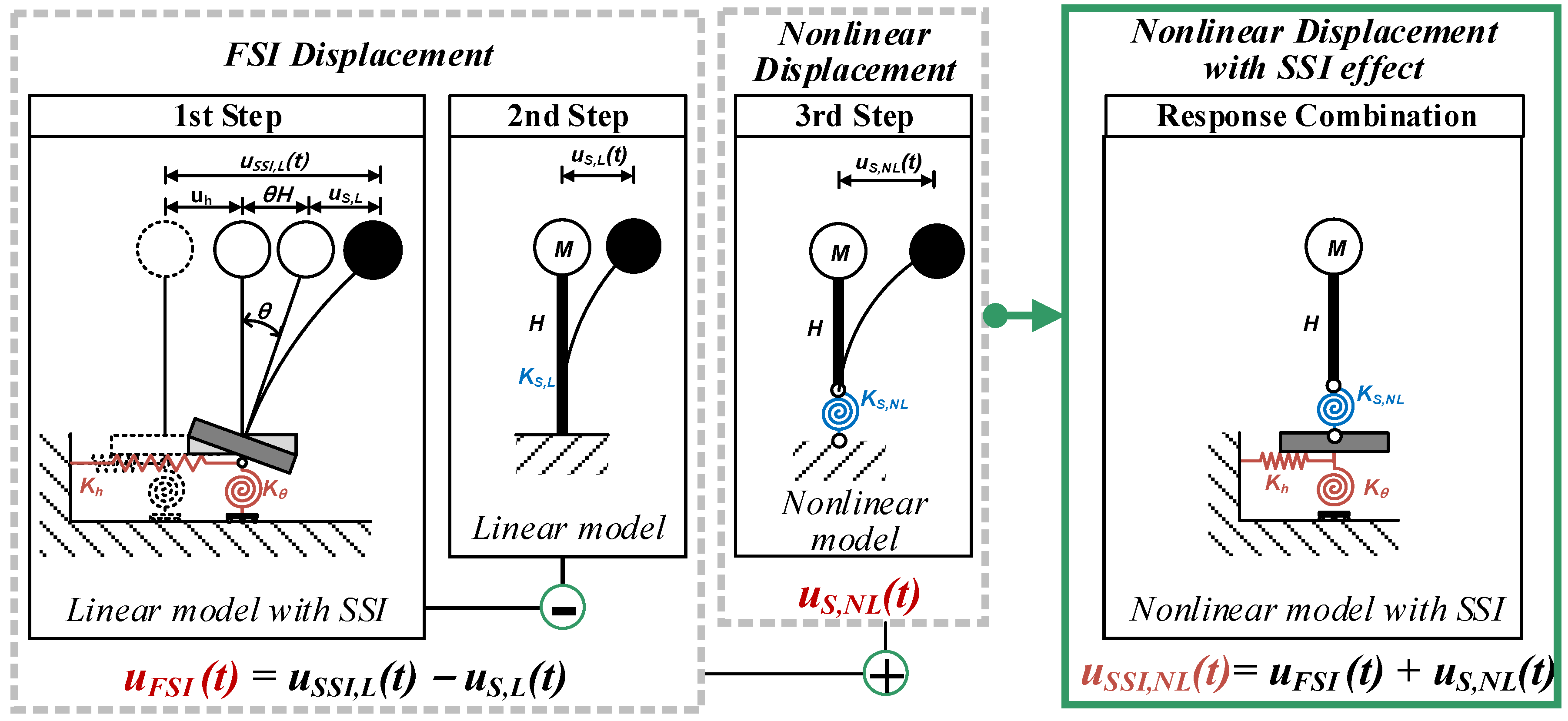
2.2. Nonlinear Displacement of Structure with SSI

To simply estimate nonlinear responses of a structure with SSI effects (u_SSI,NL), this study proposed three-step analysis procedures using SDOF models. Figure 1 summarizes the proposed procedure computing the u_SSI,NL. The first step was to compute the linear seismic response with the SSI effect using the frequency domain method as mentioned in Section 2.1. The linear SDOF model with the foundation effects used in the first step can analyze structural responses with the horizontal swaying displacement of foundation (u_h), and rocking displacement of foundation (u_θ) as presented in Figure 1. After that, the frequency domain analysis for the linear SDOF model without the foundation model was performed, and the linear structural response (u_S,L) was utilized to find the displacement of the foundation model (u_FSI = u_h + u_θ) by subtracting the u_SSI (=u_FSI + u_S,L) from the u_S,L response. Thus, the u_FSI response was the pure foundation–soil interaction (FSI) effect without the linear response of structural responses. In the next step, the nonlinear seismic response (u_S,NL) of the structure only was computed from nonlinear time–history analyses for a nonlinear SDOF structural model using OpenSees software [29]. The nonlinear SDOF model was simply developed using the rigid element and the lumped mass. The model’s nonlinear behavior was reproduced using the nonlinear rotational spring (K_S,NL), which can capture the structural damage responses, such as strength reduction, stiffness degradations, and structural collapse. In the final step, the u_SSI,NL response was computed by combining the u_S,NL with u_FSI responses. Figure 1 illustrates the seismic responses of the entire processes proposed in this study as an example and schematically compares the structural responses with the SSI effect and without the SSI effect. As shown in Figure 2, the maximum displacement of the u_SSI,NL is approximately 42.2% higher than that of the u_S,NL. Using the abovementioned approach, it was found that the SSI effect significantly affects the entire structural responses.

3. Database Construction

3.1. Reference Building Structure

In this study, a three-story, three-bay nonductile RC frame designed by ACI 318-63 [30] was selected as a reference building. The selected building frame was assumed to be located on stiff soil conditions (S_D) [31]. Figure 3 shows brief information on the structural model used in this study.

The building model is vulnerable to shear failure due to its seismically deficient detailing, such as a low transverse reinforcing bar ratio, and 90-degree L-shaped corner hooks that led to poor concrete confinement. In the analytical model, the concrete compressive strength (f_c′) of 25.9 MPa and rebar yield strength (f_y) of 303.4 MPa with 0.5% strain hardening ratio were used in this model. The masses of the frame were lumped at beam-column joint nodes in each story level. The lumped masses were computed with the load combination DL + 0.25LL, where DL = dead load and LL = live load. The self-weight (DL) was calculated based on the cross-section of each element and element length with the assumed density of concrete material (≈2400 kg/m³). The effective mass (M_eff) of the building model was approximately 193.60 N-s²/mm. More detailed information on the building model can be found in [32].

To derive the structural properties of the building model, this study performed eigenvalue and nonlinear pushover analyses. For the eigenvalue analysis, the model’s periods (T₁, and T₂) for the first and second modes are 0.46 and 0.11 s, respectively, and the mass participation ratio is 90.2% for the first mode and 8.30% for the second mode. Therefore, it was found that the building model was governed by the first mode. The normalized mode vector of the reference model in the first mode is 0.73, 0.88, and 1.0 for first-, second- and third-story, respectively. Figure 3b shows a nonlinear pushover curve of the reference model with an idealized curve. The idealized force–displacement curve was derived as specified in Federal Emergency Agency (FEMA) 356 [33]. The idealized curve was utilized to compute the structural parameters at yielding and ultimate conditions. The structural parameters include yielding strength (V_y), yielding, and ultimate displacement (Δ_y and Δ_u). The Δ_u was calculated at the point where the ultimate strength (V_u) was reduced by 20%. To implement the building model into the nonlinear SDOF model, the structural parameters obtained from the pushover analysis were transformed to a yielding spectral acceleration (S_ay) using Equation (3a), and displacement ductility capacity (μ) using Equation (3b), (for flexure-shear failure mode, S_ay = 0.62 g and μ = 2.33). Based on the structural parameters, the structural input parameters representing the nonlinear behavior were determined in Section 3.2.

$$S_{ay}=V_y/M_{eff}$$

(3a)

$$\mu ={\Delta }_u/{\Delta }_y$$

(3b)

3.2. Main Parameters in the Database

3.2.1. Input Parameters

To build the ANN model from generated nonlinear responses with the SSI effects, this study established a dataset with input and output parameters. The 11 input parameters were selected to represent earthquake excitation, nonlinear response of the structure, and geotechnical parameters as summarized in Table 1. The past earthquake records were collected from the Next Generation Attenuation (NGA) strong ground motion database [34]. Among a large amount of the past records provided by Pacific Earthquake Engineering Research (PEER), this study randomly selected 1288 ground motions measured at the S_D soil condition (S_D soil condition represents stiff soil). The reason for choosing the S_D soil condition in this study is that the current building design code [31] allowed structural engineers to select default site class as the S_D soil condition if the geotechnical information (e.g., average standard penetration test blow count, effective shear wave velocity for site soil conditions, and average undrained shear strength) is not insufficient. Additionally, the 3000 earthquake records were collected from the PEER strong ground motion database to consider the various characteristics of the ground motions. Among the collected ground motions, the authors filtered out the 1288 records measured at the S_D soil condition. The number of the earthquake records was determined to enhance the accuracy of the learning model and avoid the overfitting issue on the learning model. For the input parameters of the earthquake excitations, the earthquake magnitude (M_w), epicenter distance (ED) from the site of the structure, and the peak ground acceleration (PGA), peak ground velocity (PGV), and peak ground displacement (PGD) were selected. In addition, post-yielding stiffness (α₁), stiffness degradation ratio (α₂), and displacement ductility capacity (µ) were selected as the nonlinear structural parameters as illustrated in Figure 4. This enabled considering the various types of failure modes (e.g., shear, flexure-shear, and flexure failure modes). The upper and lower limit values of the structural parameters were determined based on the capacity curves specified in FEMA-P440A [35] and HAZUS-MH 2.1 [14]. The T and S_ay (Equation (3a)) values were fixed (T = 0.46, and S_ay = 0.62 g) based on the analytical results of the reference model as mentioned in Section 3.1.

The Poisson’s ratio (ν) and shear wave velocity (V_s) of soil ranged from 0.15 to 0.5 and ranged from 90 to 760 m/s, and were selected to cover soft clay (high ν and low V_s) to dense sand (low ν and high V_s) [31,36,37]. In addition, a shallow circular foundation was assumed in this study with a range of 0.09 to 0.7 for the ratio of structure to foundation mass.

Table 1. Summary of Input Parameter.

Input Parameters		Model Range		Note
		Minimum	Maximum
Earthquake	Mw	4.27	7.90	1288 ground motions
	ED (km)	0.44	413.33
	PGA (g)	0.01	1.64
	PGV (cm/s)	0.13	121.69
	PGD (cm)	0.01	81.78
Structure	α1	0.001	0.1	Nonlinear parameters for various failure types
	α2	−0.01	−1.25
	μ	0.80	4.00
Soil and foundation	η	0.09	0.70	Chuanromanee et al. [38]
	ν	0.15	0.50	Ganjavi et al. [36]
	Vs (m/s)	180.33	359.50	IBC [31]

M_w = earthquake magnitude; ED = epicenter distance; PGA = peak ground acceleration; PGV = peak ground velocity; PGD = peak ground displacement; α₁ = post-yielding stiffness; α₂ = strength degradation ratio; μ = displacement ductility capacity; η = ratio of structural mass to foundation mass; ν = Poisson’s ratio of soil; and V_s = shear wave velocity of soil.

Table 1. Summary of Input Parameter.

Input Parameters		Model Range		Note
		Minimum	Maximum
Earthquake	Mw	4.27	7.90	1288 ground motions
	ED (km)	0.44	413.33
	PGA (g)	0.01	1.64
	PGV (cm/s)	0.13	121.69
	PGD (cm)	0.01	81.78
Structure	α1	0.001	0.1	Nonlinear parameters for various failure types
	α2	−0.01	−1.25
	μ	0.80	4.00
Soil and foundation	η	0.09	0.70	Chuanromanee et al. [38]
	ν	0.15	0.50	Ganjavi et al. [36]
	Vs (m/s)	180.33	359.50	IBC [31]

M_w = earthquake magnitude; ED = epicenter distance; PGA = peak ground acceleration; PGV = peak ground velocity; PGD = peak ground displacement; α₁ = post-yielding stiffness; α₂ = strength degradation ratio; μ = displacement ductility capacity; η = ratio of structural mass to foundation mass; ν = Poisson’s ratio of soil; and V_s = shear wave velocity of soil.

To cover the ranges of the structural and geotechnical parameters, 10 steps of each parameter were randomly sampled using a uniform distribution from minimum to maximum values presented in Table 1. The structural parameters were randomly linked to the geotechnical parameters to build the numerical models with the SSI effects. These models were simulated under 1288 earthquake records based on the multistep analysis method. Thus, the total number of the random samples for the development of a machine-learning model was 12,880 (=10 × 1288) to find u_SSI,NL responses following the multistep analysis procedure proposed in Section 2.2.

3.2.2. Output Parameter

The u_SSI,NL response produced from the multistep analysis procedure considering the SSI effects was used to calculated the peak interstory drift ratio (IDR), which was selected as an output parameter. The evaluated IDR can be utilized to determine the seismic performance of structures by the drift-based performance limits documented in FEMA-356 [33] as given in

Table 2. Drift-based Performance Limit States.

Performance Level	Drift Limits (%)	Damage Conditions
Immediate occupancy (IO)	IDR ≤ 1.0	Minor hairline cracking; no crushing
Life safety (LS)	1.0 < IDR ≤ 2.0	Minor spalling in non-ductile column, joint cracks < 3.2 mm
Collapse prevention (CP)	2.0 < IDR ≤ 4.0	Splice failure in some non-ductile columns
Collapse (C)	IDR > 4.0	Building collapse

. Through the multistep analysis procedure, the 12,880 output responses for the u_SSI,NL were generated, and the seismic performance levels were determined using the peak IDR values computed from the u_SSI,NL. Among the entire sample data, the 2576 sample data overestimated due to numerical instability during the nonlinear-time history analyses was filtered out from the input and output datasets. Through the multistep analysis procedure, this study developed 10,304 datasets for training, validating, and testing a machine-learning model.

4. ANN-Based Rapid-Decision Making Model

4.1. Development of ANN Model

In the past decades, the growing use of ANN in engineering increased the applicability of this brain-inspired technique to solve many engineering problems with the nonlinear relationship between input and output [39]. The ANN structure is composed of the input layer, zero or more hidden layers, and output layer, which are interconnected by multiple nodes in each layer as illustrated in Figure 5. The value of neurons at the immediately following layer of the input layer (x_j) is expressed as:

$$x_j=f(\overline{a_i})=f({\displaystyle \sum _j{w}_{ij}{x}_i-\overline{b})}$$

(4)

where i is the immediately preceding layer of j layer, j is the immediately following layer of i layer, x_i is the input value in the neuron, f(•) is transfer or activation function, w_ij is weight coefficient that represents the degree of importance of the connection between the ith and jth neurons, ${\displaystyle \sum _j{w}_{ij}{x}_i}$ = weighted summation, and $\overline{b}$ = threshold or bias value in the associated neuron. The neural network approach is based on a supervised process, which knows actual (target) outputs for the inputs utilized in the model training and provides predicted outputs by comparing the target and predicted outputs. The errors between the target and predicted values are minimized by the learning algorithms, such as back-propagation, Quasi-Newton and Levenberg–Marquardt algorithms. By using the learning algorithms, the weight and bias values of the multiple hidden and output layers are automatically found.

Figure 6 illustrates the ANN structure developed in this study to produce the peak IDR with the SSI effects. The model was constructed with the 11 input and 1 output parameter as described in Section 3. The neural network model used in this study was composed of multiple hidden layers: two nine-hidden layers and one four-hidden layer, and one two-hidden layer. The number of the hidden layers was determined using the trial-and-error method until the ANN model ensured more than 80% accuracy. As illustrated in Figure 6, a linear transfer function was assigned to the first hidden layer and the output layer, and a log-sigmoid transfer function was utilized to the remaining hidden layers. To solve the nonlinear problem, this study utilized the Levenberg–Marquardt Algorithm (LMA) in the neural network model as the learning algorithm, which provides the best-fit values of the w and $\overline{b}$ parameters in the activation functions to minimize the mean squared error (MSE) in an iterative process.

4.2. Model Training, Validation, and Testing

This study randomly split the entire dataset into 70% for a training set, 10% for a validation set, and 20% for a testing set. The training set was utilized to develop the ANN model using the structure given in Figure 7, and the validation set was to tune the hyper-parameters of the ANN model and to prevent overfitting issues of the ANN model in the training process. The testing set was used to estimate the accuracy of the ANN model. This study trained, validated, and tested the ANN model using 10,304 sample data (8115 for the training set, 1159 for the validation set, and 2318 for the testing set) excluding 2576 sample data, filtered out due to the numerical instability. Since input and output parameters follow the lognormal distribution, this study adopted the natural logarithm to the input and output parameters for training, validation, and testing.

Figure 7 shows the MSE values for an entire iteration process. The MSE value was utilized to estimate the performance of the ANN model in this study. The MSE values computed in each iteration step were the average of the squared error between predicted (Y) and target (T) values:

$$MSE=\frac{1}{n}{\displaystyle \sum _{i=1}^n{(Y_i-T_i)}^2}$$

(5)

where n = the number of samples; Y_i = ith predicted value; and T_i = ith target value. As shown in Figure 7, the training of the ANN model was stopped at the 129th iteration step where the MSE was minimized, where the values of the MSE for the training, validation and testing sets are estimated as 0.003, 0.004, and 0.005, respectively. The difference between the MSE-values between the training and testing sets was negligible.

In addition, the performance of the ANN model was evaluated by a simple regression model, Y = T regression model. The regression model can judge the correlation between the Y- and T-values. Figure 8 shows the relationship between the Y and T values for the training, validation, testing datasets, and the entire dataset with the coefficient of determination (R²) values. The R² can be evaluated as:

$$R^2=1-\frac{{\displaystyle {\sum }_{i=1}^n}{(Y_i-T_i)}^2}{{\displaystyle {\sum }_{i=1}^n}{(Y_i-\overline{Y})}^2}$$

(6)

where $\overline{Y}$ is the mean of the predicted values.

As shown in Figure 8, the R² values for the training, validation, testing, and entire datasets were approximately 0.98, 0.96, 0.96, and 0.97. This indicates that the Y values are highly correlated to the T values predicted from the ANN model. Since the R² values for the validation and testing datasets are marginally different from the R² value for the training dataset, the ANN model was well-developed without the overfitting issue.

The confusion matrix was evaluated in this study to estimate the classification of the seismic performance levels from the developed ANN model. The evaluated target and predicted peak IDR values were utilized to build a confusion chart, which enables the developed ANN model’s accuracy for classifying the seismic performance levels by Drift-based Performance Limit States in Table 2. Thus, the off-diagonal elements in Figure 9 and Figure 10 represent the failure of predicting the seismic performance level by the developed ANN model. The accuracy of the ANN model for the classification problem defines the ratio of the number of successful predictions over the total number of samples.

On average of 4 levels (IO, LS, CP, and collapse), the accuracy of the developed ANN model was 85.6% for the training dataset and 83.71% for the testing dataset. Notably, the accuracy of IO level was extremely high (99.7% and 99.8% for training and testing dataset) while the lowest accuracy was observed for CP level for the training dataset and collapse level for testing dataset. Overall, the accuracy of the developed ANN model decreases as peak IDR values increase. However, the accuracy of 83.71% for the testing dataset indicates that the developed ANN model in this study satisfied the target performance (>80%). The larger dataset would be required to increase the model accuracy at high IDR values. The investigation of the ANN model’s performance (e.g., MSE and R² values, and confusion matrix) demonstrated that the developed ANN model by generated the Peak IDR responses with the SSI effects is well-trained without the overfitting issues, and the accuracy of the ANN model satisfied the target accuracy.

4.3. ANN-Based Rapid Decision-Making Tool

This section presents the potential use of the developed ANN model (with >80% accuracy) as a rapid decision-making tool for determining the seismic performance levels. The peak IDR responses were generated by the developed ANN model without the analytical modeling of the building structures and multistep analysis procedure described in Section 2.2. Figure 11 presents the 4000 data points among 50,000 evaluated peak IDR values with respect to 50,000 sets of randomly generated input parameters. Figure 11 provides the fraction of performance levels at a given range of structure-related and geotechnical input parameters used in this study. Notably, to produce the 50,000 reliable responses using the ANN model, about 3 min were taken using a computer with 3.00 GHz CPU and 8 GB RAM. This indicates that the proposed framework in this study for developing the ANN model substantially reduced the computational time compared to the traditional FE models.

The most and the second most important structure-related and geotechnical input parameters were selected as parameters on the x and y-axis in Figure 11, which were determined by the Relief algorithm. The Relief algorithm has been widely used to analyze the impact of input parameters on the output by computing the weights of the multiple variables, which represent the importance of input parameters. The use of a Relief algorithm in this study showed that the μ and α₂ parameters for the structural parameters and the η and V_s for the geotechnical parameters were significantly affected to the peak IDR.

5. Conclusions

This study proposed the framework of developing the ANN model for predicting the seismic performance levels of the building structure with soil–structure interaction effects. The soil–structure interaction effect was incorporated into the single-degree-of-freedom model by a proposed three-step analysis, and 11 input parameters were selected to account for the characteristics of the earthquake, nonlinear behavior of the structure, and soil characteristics. Unlike the ANN-based models in previous studies, the developed framework presented in this study enables incorporating SSI effects in the model. The ratio of structural mass to foundation mass (η), shear wave velocity (V_s), and Poisson’s ratio (υ) can be reflected in the model in addition to structural and earthquake-related parameters. Based on the performance and the application of the developed ANN model, the following conclusions can be drawn:

(1)

The proposed three-step analysis provides the methodology for generating the dataset for nonlinear response in the SDOF system with the consideration of SSI effects. The proposed analysis is anticipated to be used for investigating the nonlinear response in the MDOF system or FEM-based results.

(2)

Evaluated MSE, R² values and confusion matrix indicate that the developed ANN model in this study showed more than 80% accuracy without any overfitting issues. In addition, the confusion matrix presented in this study can be an efficient method to evaluate the accuracy of the developed model in each seismic performance level.

(3)

The developed ANN model can rapidly generate an extensive database and determine the drift-based performance levels within a training range of the input parameters. Furthermore, using the developed ANN model significantly reduced computational time to generate large datasets compared to the traditional FE models. Since the ANN model can rapidly generate reliable responses using brief structural and geotechnical information without any complex modeling processes, the model can be a useful alternative to the seismic damage assessment on a regional level for safe and sustainable structures.

References

1. El-Betar, S.A. Seismic performance of existing RC framed buildings. HBRC J. 2017, 13, 171–180. [Google Scholar] [CrossRef] [Green Version]
2. Pelekis, I.; Madabhushi, G.S.P.; DeJong, M.J. Seismic performance of buildings with structural and foundation rocking in centrifuge testing. Earthq. Eng. Struct. Dyn. 2018, 47, 2390–2409. [Google Scholar] [CrossRef] [Green Version]
3. Stewart, J.P.; Fenves, G.L.; Seed, R.B. Seismic soil-structure interaction in buildings. I: Analytical methods. J. Geotech. Geoenviron. Eng. 1999, 125, 26–37. [Google Scholar] [CrossRef]
4. Stewart, J.P.; Seed, R.B.; Fenves, G.L. Seismic soil-structure interaction in buildings. II: Empirical findings. J. Geotech. Geoenviron. Eng. 1999, 125, 38–48. [Google Scholar] [CrossRef] [Green Version]
5. Seed, R.B.; Dickenson, S.E.; Mok, C.M. Recent lessons regarding seismic response analysis of soft and deep clay sites. In Technical Report NCEER; US National Center for Earthquake Engineering Research (NCEER): Alachua, FL, USA, 1992; pp. 131–145. [Google Scholar]
6. Torabi, H.; Rayhani, M.T. Three dimensional finite element modeling of seismic soil–structure interaction in soft soil. Comput. Geotech. 2014, 60, 9–19. [Google Scholar] [CrossRef]
7. Kim, D.K. Effects of Shallow Soil Deposits and Substructures on Earthquake Response Spectrum. Ph.D. Dissertation, Seoul National University, Seoul, Korea, 2013. [Google Scholar]
8. Karimi, Z.; Dashti, S. Numerical and centrifuge modeling of seismic soil–foundation–structure interaction on liquefiable ground. J. Geotech. Geoenviron. Eng. 2016, 142, 4015061. [Google Scholar] [CrossRef]
9. Cubrinovski, M.; Bray, J.D.; Taylor, M.; Giorgini, S.; Bradley, B.; Wotherspoon, L.; Zupan, J. Soil liquefaction effects in the central business district during the February 2011 Christchurch earthquake. Seismol. Res. Lett. 2011, 82, 893–904. [Google Scholar] [CrossRef]
10. Gihm, Y.S.; Kim, S.W.; Ko, K.; Choi, J.-H.; Bae, H.; Hong, P.S.; Lee, Y.; Lee, H.; Jin, K.; Choi, S.J. Paleoseismological implications of liquefaction-induced structures caused by the 2017 Pohang earthquake. Geosci. J. 2018, 22, 871–880. [Google Scholar] [CrossRef]
11. Barbat, A.H.; Pujades, L.G.; Lantada, N. Performance of buildings under earthquakes in Barcelona, Spain. Comput. Aided Civ. Infrastruct. Eng. 2006, 21, 573–593. [Google Scholar] [CrossRef]
12. MAE Center. Earthquake Risk Assessment Using MAEviz 2.0: A Tutorial; Mid-America Earthquake Center, University of Illinois at Urbana-Champaign: Urbana-Champaign, IL, USA, 2006.
13. Hori, M.; Ichimura, T. Current state of integrated earthquake simulation for earthquake hazard and disaster. J. Seismol. 2008, 12, 307–321. [Google Scholar] [CrossRef]
14. Federal Emergency Management Agency. Multi-Hazard Loss Estimation Methodology Earthquake Model Hazus®-MH 2.1 Technical Manual; Federal Emergency Management Agency: Washington, DC, USA, 2016.
15. Seo, J.; Hu, J.W.; Davaajamts, B. Seismic performance evaluation of multistory reinforced concrete moment resisting frame structure with shear walls. Sustainability 2015, 7, 14287–14308. [Google Scholar] [CrossRef] [Green Version]
16. Dang-Vu, H.; Shin, J.; Lee, K. Seismic Fragility Assessment of Columns in a Piloti-Type Building Retrofitted with Additional Shear Walls. Sustainability 2020, 12, 6530. [Google Scholar] [CrossRef]
17. Dashti, S.; Bray, J.D. Numerical simulation of building response on liquefiable sand. J. Geotech. Geoenviron. Eng. 2013, 139, 1235–1249. [Google Scholar] [CrossRef]
18. Hokmabadi, A.S.; Fatahi, B. Influence of foundation type on seismic performance of buildings considering soil–structure interaction. Int. J. Struct. Stab. Dyn. 2016, 16, 1550043. [Google Scholar] [CrossRef]
19. Luque, R.; Bray, J.D. Dynamic soil-structure interaction analyses of two important structures affected by liquefaction during the Canterbury earthquake sequence. Soil Dyn. Earthq. Eng. 2020, 133, 106026. [Google Scholar] [CrossRef]
20. Van Nguyen, Q.; Fatahi, B.; Hokmabadi, A.S. Influence of size and load-bearing mechanism of piles on seismic performance of buildings considering soil–pile–structure interaction. Int. J. Geomech. 2017, 17, 4017007. [Google Scholar] [CrossRef]
21. Cha, Y.; Choi, W.; Büyüköztürk, O. Deep learning-based crack damage detection using convolutional neural networks. Comput. Aided Civ. Infrastruct. Eng. 2017, 32, 361–378. [Google Scholar] [CrossRef]
22. Cha, Y.; Choi, W.; Suh, G.; Mahmoudkhani, S.; Büyüköztürk, O. Autonomous structural visual inspection using region-based deep learning for detecting multiple damage types. Comput. Aided Civ. Infrastruct. Eng. 2018, 33, 731–747. [Google Scholar] [CrossRef]
23. ATC Goh. Nonlinear modelling in geotechnical engineering using neural networks. Trans. Inst. Eng. Aust. Civ. Eng. 1994, 36, 293–297. [Google Scholar]
24. ATC Goh. Empirical design in geotechnics using neural networks. Géotechnique 1995, 45, 709–714. [Google Scholar] [CrossRef]
25. Alavi, A.H.; Gandomi, A.H. Prediction of principal ground-motion parameters using a hybrid method coupling artificial neural networks and simulated annealing. Comput. Struct. 2011, 89, 2176–2194. [Google Scholar] [CrossRef]
26. Kia, A.; Şensoy, S. Assessment the Effective Ground Motion Parameters on Seismic Performance of R/C Buildings Using Artificial Neural Network; Indian Society for Education and Environment: Chennai, India, 2014. [Google Scholar]
27. Lagaros, N.D.; Papadrakakis, M. Neural network based prediction schemes of the non-linear seismic response of 3D buildings. Adv. Eng. Softw. 2012, 44, 92–115. [Google Scholar] [CrossRef]
28. Lu, Y. Seismic Soil-Structure Interaction in Performance-Based Design. Ph.D. Dissertation, University of Nottingham, Nottingham, UK, 2016. [Google Scholar]
29. McKenna, F.; Scott, M.H.; Fenves, G.L. Nonlinear finite-element analysis software architecture using object composition. J. Comput. Civ. Eng. 2010, 24, 95–107. [Google Scholar] [CrossRef]
30. ACI Committee. Building Code Requirements for Reinforced Concrete (ACI 318-63); American Concrete Institute: Farmington Hills, MI, USA, 1963. [Google Scholar]
31. IBC. International Code Council; International Building Code: Washington, DC, USA, 2018. [Google Scholar]
32. Shin, J.; Jeon, J.S.; Kim, J. Mainshock-aftershock response analyses of FRP-jacketed columns in existing RC building frames. Eng. Struct. 2018, 165, 315–330. [Google Scholar] [CrossRef]
33. Federal Emergency Management Agency. Prestandard and Commentary for the Seismic Rehabilitation of Buildings; Report FEMA 356; Federal Emergency Management Agency: Washington, DC, USA, 2000.
34. Ancheta, T.D.; Darragh, R.B.; Stewart, J.P.; Seyhan, E.; Silva, W.J.; Chiou, B.S.-J.; Wooddell, K.E.; Graves, R.W.; Kottke, A.R.; Boore, D.M. NGA-West2 database. In Earthquake Spectra; SAGE Publications Sage UK: London, UK, 2014; Volume 30, pp. 989–1005. [Google Scholar] [CrossRef]
35. Federal Emergency Management Agency. Effects of Strength and Stiffness Degradation on Seismic Response; Report FEMA 440a; Federal Emergency Management Agency: Washington, DC, USA, 2009.
36. Ganjavi, B.; Hajirasouliha, I.; Bolourchi, A. Optimum lateral load distribution for seismic design of nonlinear shear-buildings considering soil-structure interaction. Soil Dyn. Earthq. Eng. 2016, 88, 356–368. [Google Scholar] [CrossRef]
37. Payan, M.; Senetakis, K.; Khoshghalb, A.; Khalili, N. Effect of gradation and particle shape on small-strain Young’s modulus and Poisson’s ratio of sands. Int. J. Geomech. 2018, 17, 4016120. [Google Scholar] [CrossRef] [Green Version]
38. Chuanromanee, O.; Hanson, R.D.; Woods, R.D. The influence of soil-structure interaction on the overall damping of structures with high damping. In WIT Transactions on the Built Environment; WIT Press: Chilworth, UK, 1970. [Google Scholar]
39. Cao, M.S.; Pan, L.X.; Gao, Y.F.; Novák, D.; Ding, Z.C.; Lehký, D.; Li, X.L. Neural network ensemble-based parameter sensitivity analysis in civil engineering systems. Neural Comput. Appl. 2017, 28, 1583–1590. [Google Scholar] [CrossRef]
Figure 1. Proposed method for generating a nonlinear structural response with soil−structure interaction (SSI) effect.
Sustainability 13 04334 g001
Figure 2. Time series nonlinear structural response with SSI effect using the proposed method.
Sustainability 13 04334 g002
Figure 3. Information on Reference Building. Note that b = width of element; h = depth of element; s = spacing of column ties or beam stirrups, ρl = longitudinal reinforcement ratio; and ρt = transverse reinforcement ratio.
Sustainability 13 04334 g003
Figure 4. Structural Input Parameters.
Sustainability 13 04334 g004
Figure 5. Typical Structure of artificial neural network.
Sustainability 13 04334 g005
Figure 6. Artificial neural network structure developed in this study.
Sustainability 13 04334 g006
Figure 7. Mean squared error (MSE)−based artificial neural network (ANN) Model’s performance.
Sustainability 13 04334 g007
Figure 8. Relationships between predicted (Y) and target (T) values: (a) training dataset; (b) validation dataset; (c) testing dataset; and (d) entire dataset.
Sustainability 13 04334 g008
Figure 9. Confusion matrix for training dataset.
Sustainability 13 04334 g009
Figure 10. Confusion matrix for testing dataset.
Sustainability 13 04334 g010
Figure 11. Multiple parameter-peak interstory drift ratio (IDR) relationships predicted from ANN model: (a) structure-related parameters; and (b) geotechnical parameters.
Sustainability 13 04334 g011