
Regional-Scale Landslide Susceptibility Mapping Using Limited LiDAR-Based Landslide Inventories for Sisak-Moslavina County, Croatia


Abstract
:1. Introduction
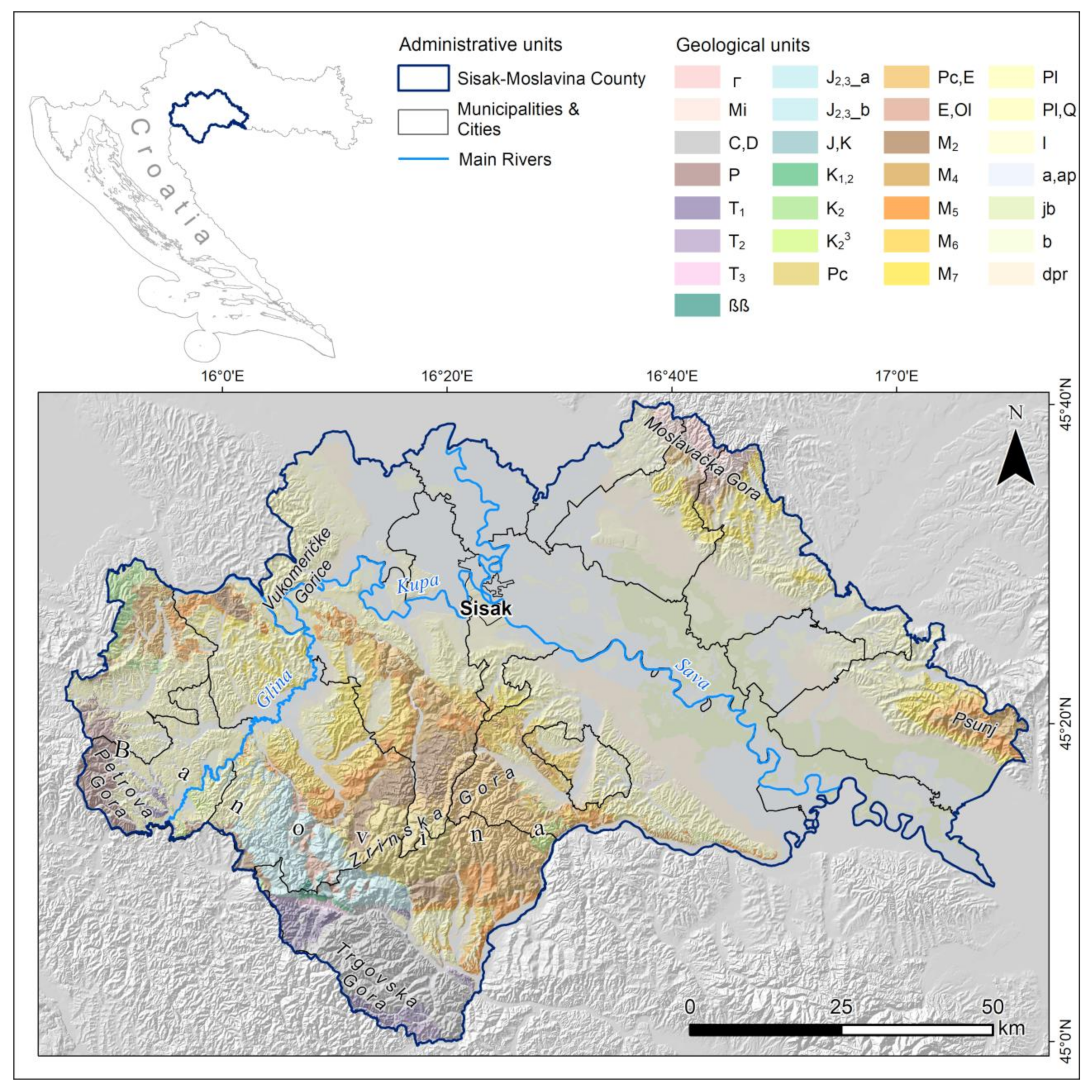
2. Study Area
Geological Setting and Description of Geological Units
3. Materials and Methods
3.1. Datasets
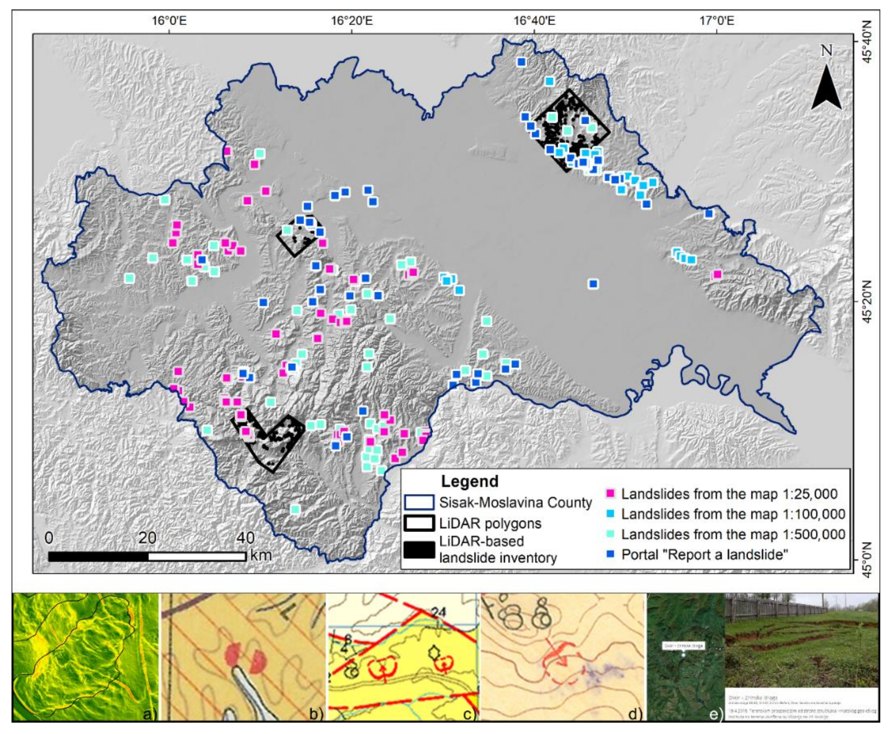
3.1.1. Landslide Inventories
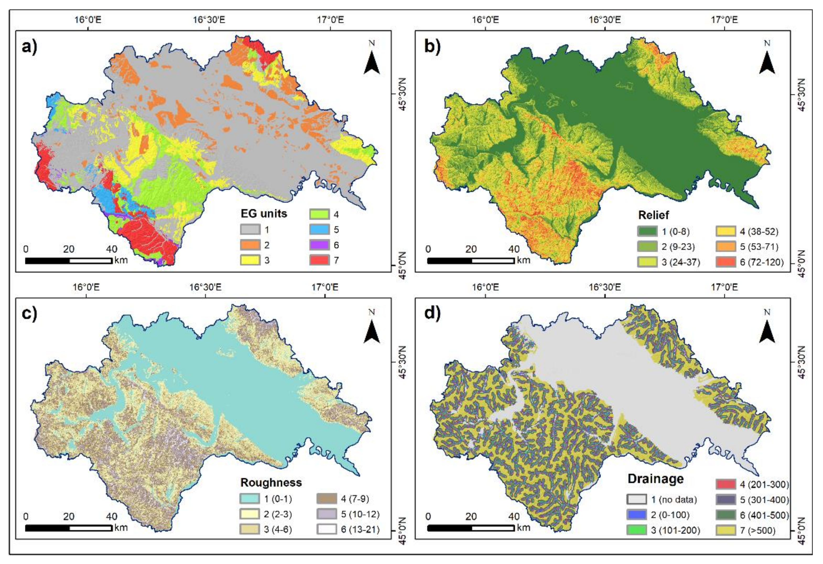
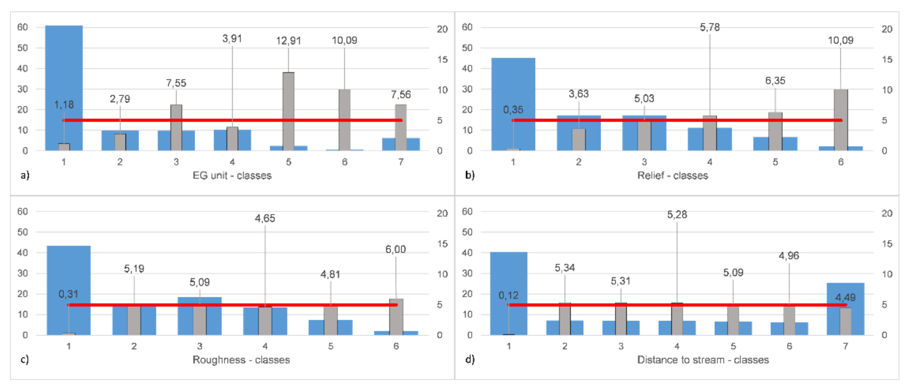
3.1.2. Landslide Predictive Factors
EG Units
Relief
Roughness
Distance to Streams
3.2. Analytical Methods
4. Results and Discussion
4.1. The Weighting of Predictive Factors
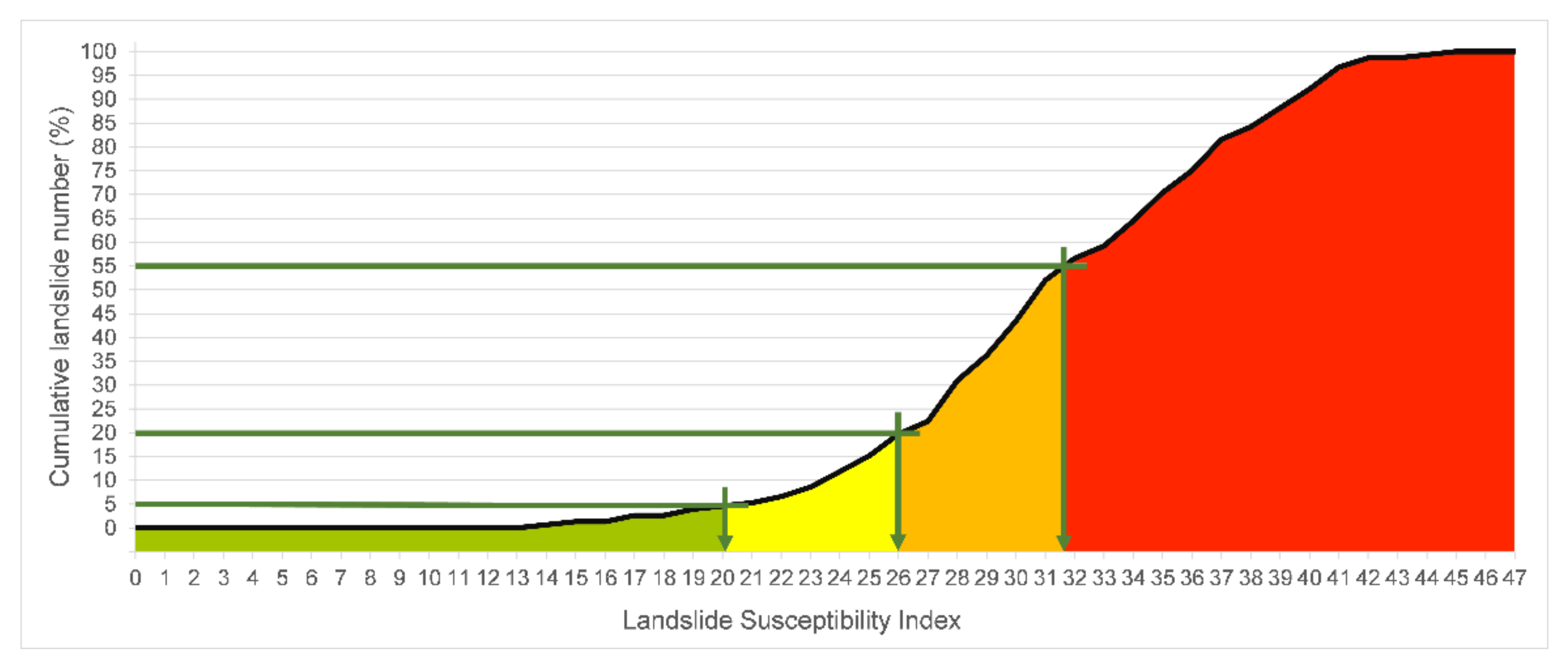
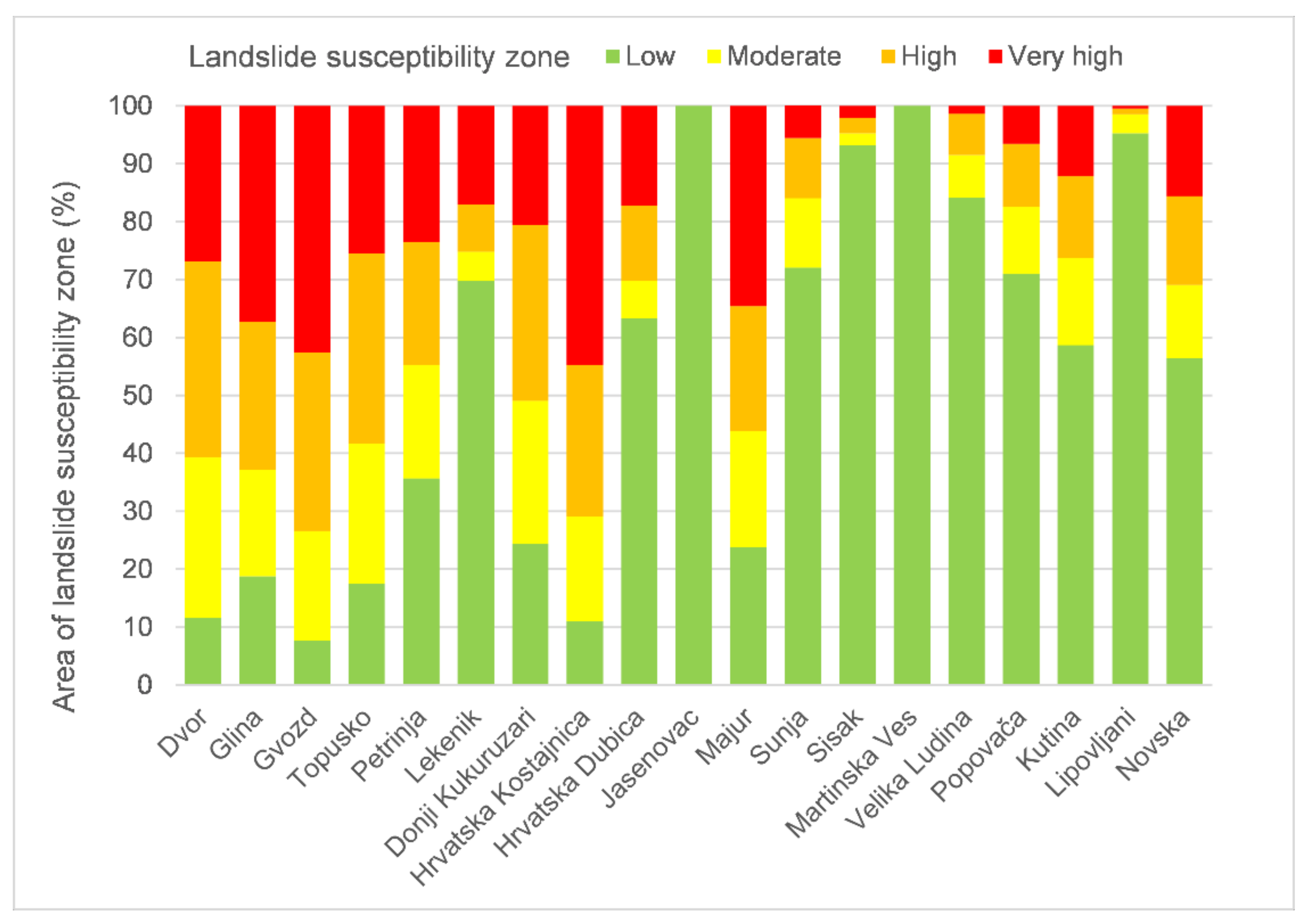
4.2. Landslide Susceptibility Map and Verification
4.3. Limitations
4.4. Purpose and Method of Use
5. Conclusions
Author Contributions
Funding
Institutional Review Board Statement
Informed Consent Statement
Data Availability Statement
Acknowledgments
Conflicts of Interest
References
- Schuster, R.L. Socioeconomic Significance of Landslides. In Landslides—Investigation and Mitigation; Turner, A.K., Schuster, R.L., Eds.; Transportation Research Board Special Report; National Academy Press: Washington, DC, USA, 1996; Volume 247, pp. 12–35. [Google Scholar]
- Crozier, M.J. Deciphering the Effect of Climate Change on Landslide Activity: A Review. Geomorphology 2010, 124, 260–267. [Google Scholar] [CrossRef]
- Gariano, S.L.; Guzzetti, F. Landslides in a Changing Climate. Earth-Sci. Rev. 2016, 162, 227–252. [Google Scholar] [CrossRef] [Green Version]
- Bell, F.G. Geological Hazards: Their Assessment, Avoidance and Mitigation; Taylor & Francis e-Library: London, UK, 2002. [Google Scholar]
- Hervas, J.; Bobrowsky, P.T. Mapping: Inventories, Susceptibility, Hazard and Risk. In Landslides—Disaster Risk Reduction; Sassa, K., Canuti, P., Eds.; Springer: Berlin, Germany, 2009; pp. 321–349. [Google Scholar] [CrossRef]
- Corominas, J.; Van Westen, C.; Frattini, P.; Cascini, L.; Malet, J.-P.; Fotopoulou, S.; Catani, F.; Van Den Eeckhaut, M.; Mavrouli, O.; Agliardi, F.; et al. Recommendations for the Quantitative Analysis of Landslide Risk. Bull. Eng. Geol. Environ. 2014, 73, 209–263. [Google Scholar] [CrossRef]
- Brabb, E.E. Innovative approaches to landslide hazard and risk mapping. In Proceedings of the 4th International Symposium on Landslides, Toronto, ON, USA, 16–21 September 1984; Canadian Geotechnical Society: Toronto, ON, Canada, 1984; Volume 1, pp. 307–324. [Google Scholar]
- Chacón, J.; Irigaray, C.; Fernández, T.; El Hamdouni, R. Engineering Geology Maps: Landslides and Geographical Information Systems. Bull. Eng. Geol. Environ. 2006, 65, 341–411. [Google Scholar] [CrossRef]
- Fell, R.; Corominas, J.; Bonnard, C.; Cascini, L.; Leroi, E.; Savage, W.Z. Guidelines for Landslide Susceptibility, Hazard and Risk Zoning for Land Use Planning. Eng. Geol. 2008, 102, 85–98. [Google Scholar] [CrossRef] [Green Version]
- Cascini, L. Applicability of Landslide Susceptibility and Hazard Zoning at Different Scales. Eng. Geol. 2008, 102, 164–177. [Google Scholar] [CrossRef]
- Van Westen, C.J.; Rengers, N.; Terlien, M.T.J.; Soeters, R. Prediction of the occurrence of slope instability phenomena through GIS-based hazard zonation. Geol. Rundsh. 1997, 86, 404–414. [Google Scholar] [CrossRef]
- Reichenbach, P.; Rossi, M.; Malamud, B.D.; Mihir, M.; Guzzetti, F. A Review of Statistically-Based Landslide Susceptibility Models. Earth-Sci. Rev. 2018, 180, 60–91. [Google Scholar] [CrossRef]
- Schicker, R.; Moon, V. Comparison of Bivariate and Multivariate Statistical Approaches in Landslide Susceptibility Mapping at a Regional Scale. Geomorphology 2012, 161–162, 40–57. [Google Scholar] [CrossRef]
- Manzo, G.; Tofani, V.; Segoni, S.; Battistini, A.; Catani, F. GIS Techniques for Regional-Scale Landslide Susceptibility Assessment: The Sicily (Italy) Case Study. Int. J. Geogr. Inf. Sci. 2013, 27, 1433–1452. [Google Scholar] [CrossRef]
- Ahmed, M.F.; Rogers, J.D.; Ismail, E.H. A Regional Level Preliminary Landslide Susceptibility Study of the Upper Indus River Basin. Eur. J. Remote Sens. 2014, 47, 343–373. [Google Scholar] [CrossRef] [Green Version]
- Chalkias, C.; Polykretis, C.; Ferentinou, M.; Karymbalis, E. Integrating Expert Knowledge with Statistical Analysis for Landslide Susceptibility Assessment at Regional Scale. Geosciences 2016, 6, 14. [Google Scholar] [CrossRef] [Green Version]
- Hung, L.Q.; Van, N.T.H.; Duc, D.M.; Ha, L.T.C.; Van Son, P.; Khanh, N.H.; Binh, L.T. Landslide Susceptibility Mapping by Combining the Analytical Hierarchy Process and Weighted Linear Combination Methods: A Case Study in the Upper Lo River Catchment (Vietnam). Landslides 2016, 13, 1285–1301. [Google Scholar] [CrossRef]
- Zhou, S.; Chen, G.; Fang, L.; Nie, Y. GIS-Based Integration of Subjective and Objective Weighting Methods for Regional Landslides Susceptibility Mapping. Sustainability 2016, 8, 334. [Google Scholar] [CrossRef] [Green Version]
- Du, G.L.; Zhang, Y.S.; Iqbal, J.; Yang, Z.H.; Yao, X. Landslide Susceptibility Mapping Using an Integrated Model of Information Value Method and Logistic Regression in the Bailongjiang Watershed, Gansu Province, China. J. Mt. Sci. 2017, 14, 249–268. [Google Scholar] [CrossRef]
- Milevski, I.; Dragićević, S.; Zorn, M. Statistical and Expert-Based Landslide Susceptibility Modeling on a National Scale Applied to North Macedonia. Open Geosci. 2019, 11, 750–764. [Google Scholar] [CrossRef]
- Rabby, Y.W.; Li, Y. Landslide Susceptibility Mapping Using Integrated Methods: A Case Study in the Chittagong Hilly Areas, Bangladesh. Geosciences 2020, 10, 483. [Google Scholar] [CrossRef]
- Guzzetti, F.; Mondini, A.C.; Cardinali, M.; Fiorucci, F.; Santangelo, M.; Chang, K.-T. Landslide Inventory Maps: New Tools for an Old Problem. Earth-Sci. Rev. 2012, 112, 42–66. [Google Scholar] [CrossRef] [Green Version]
- Bognar, A. Geomorfološka regionalizacija Hrvatske [The Geomorphological Regionalization of Croatia—In Croatian]. Acta Geogr. Croat. 2001, 34, 7–29. [Google Scholar]
- Husnjak, S.; Bogunović, M.; Jurišić, M. Geoinformatička obrada pedoloških podataka za uzgoj povrća na području Sisačko-Moslavačke županije [Geoinformatic Processing of Pedological Data for Vegetable Farming in the Sisak-Moslavina County—In Croatian]. Agron. Glas. 2000, 227–246. [Google Scholar]
- Sisačko-Moslavačka Županija. Izvješće o Stanju u Prostoru Sisačko-Moslavačke Županije 2015–2018; Report on the Spatial Situation in the Sisak-Moslavina County—In Croatian. Zavod za Prostorno Uređenje Sisačko-Moslavačke Županije: Sisak, Croatia, 2019; 65p. [Google Scholar]
- Bogunović, M.; Vidaček, Ž.; Racz, Z.; Husnjak, S.; Sraka, M. Namjenska pedološka karta Republike Hrvatske i njena uporaba [The Practical Aspects of Soil Suitability Map of Croatia—In Croatian]. Agron. Glas. 1997, 59, 363–399. [Google Scholar]
- Hećimović, I.; Avanić, R. Geološka Karta Sisačko-Moslavačke Županije [Geological Map of Sisak-Moslavina County—In Croatian]; Prilog br. 1 iz Rudarsko-geološke studije Sisačko-moslavačke županije [Annex No. 1 from Mining and Geological Study of Sisak-Moslavina County—In Croatian]; Croatian Geological Survey: Zagreb, Croatia, 2014. [Google Scholar]
- Kruk, B.; Dedić, Ž.; Avanić, R.; Peh, Z.; Kruk, L.; Kovačević Galović, E.; Kolbah, S.; Škrlec, M.; Crnogaj, S. Rudarsko-Geološka Studija Sisačko-Moslavačke Županije [Mining and Geological Study of Sisak-Moslavina County—In Croatian]; Department of Mineral Resources, Croatian Geological Survey: Zagreb, Croatia, 2016. [Google Scholar]
- Šikić, K. Tumač Osnovne Geološke Karte RH za List Bosanski Novi 1:100,000, L 33-105 [The Guidelines of the Basic Geological Map of the Republic of Croatia for the Sheet Bosanski Novi 1: 100,000—In Croatian]; Croatian Geological Survey: Zagreb, Croatia, 2014. [Google Scholar]
- Jelaska, V.; Bulić, J.; Oreški, E. Stratigrafski Model Eocenskog Fliša Banije [The Stratigraphic Model of the Eocene Flysch of Banija—In Croatian]. Geološki Vjesnik 1970, 23, 81–94. [Google Scholar]
- Avanić, R. Litostratigrafske Jedinice Donjeg Miocena Sjeverozapadne Hrvatske [The Lithostratigraphic Units of the Early Miocene of Northwestern Croatia—In Croatian]. Ph.D. Thesis, Faculty of Science, University of Zagreb, Zagreb, Croatia, 2012. [Google Scholar]
- Avanić, R.; Kovačić, M.; Pavelić, D.; Miknić, M.; Vrsaljko, D.; Bakrač, K.; Galović, I. The Middle and Upper Miocene Facies of Mt. Medvednica (Northern Croatia). In Proceedings of the 22nd IAS Meeting of Sedimentology; Field Trip Guidebook; Vlahović, I., Tišljar, J., Eds.; Croatian Geological Survey: Zagreb, Croatia, 2003; pp. 167–172. [Google Scholar]
- Avanić, R.; Šimunić, A.; Peh, Z. Geology of the Croatian Zagorje Region. In Proceedings of the 5th Slovenian Geological Congress; Post congress field trip book; Rman, N., Marković, T., Brenčić, M., Eds.; Geological Survey of Slovenia: Ljubljana, Slovenia, 2018; p. 35. [Google Scholar]
- Kovačić, M. Sedimentologija Gornjomiocenskih Naslaga Jugozapadnog Dijela Panonskog Bazena [Sedimentology of the Upper Miocene Deposits from the Southwest Part of the Pannonian Basin—In Croatian]. Ph.D. Thesis, Faculty of Science, University of Zagreb, Zagreb, Croatia, 2004. [Google Scholar]
- Grizelj, A. Mineraloške i Geokemijske Značajke Gornjomiocenskih Pelitnih Sedimenata Jugozapadnog Dijela Hrvatskog Zagorja [Mineralogical and Geochemical Characteristics of Upper Miocene Pelitic Sediments of the South-Western Part of Hrvatsko Zagorje—In Croatian]. Master’s Thesis, Faculty of Science, University of Zagreb, Zagreb, Croatia, 2004. [Google Scholar]
- Avanić, R.; Kovačić, M.; Pavelić, D.; Peh, Z. The Neogene of Hrvatsko Zagorje. In Proceedings of the 9th Mid-European Clay Conference; Conference book, Field Trip Guide book; Tibljaš, D., Horvat, M., Tomašić, N., Mileusnić, M., Grizelj, A., Eds.; Croatian Geological Society, Croatian Geological Survey, Faculty of Mining, Geology and Petroleum Engineering, and Faculty of Science—University of Zagreb: Zagreb, Croatia, 2018; pp. 128–129. [Google Scholar]
- Pikija, M. Tumač Osnovne Geološke Karte SFRJ za List Sisak 1:100,000 L 33-93 [The Guidelines of the Basic Geological Map of the Republic of Croatia for the Sheet Sisak 1:100,000—In Croatian]; Institut za Geološka Istraživanja, Zagreb, Savezni Geol. Zavod: Beograd, Serbia, 1986. [Google Scholar]
- Halamić, J.; Belak, M.; Pavelić, D.; Avanić, R.; Šparica, M.; Brkić, M.; Kovačić, M.; Vrsaljko, D.; Banak, A.; Crnko, J. Osnovna Geološka Karta Republike Hrvatske 1:50,000—Požeška Gora [Basic Geological Map of the Republic of Croatia 1:50,000—Požeška Gora—In Croatian]; Croatian Geological Survey: Zagreb, Croatia, 2019. [Google Scholar]
- Varnes, D.J.; IAEG. Landslide Hazard Zonation: A Review of Principles and Practice; UNESCO: Paris, France, 1984. [Google Scholar]
- Van Westen, C.J. The Modeling of Landslide Hazards Using GIS. Surv. Geophys. 2000, 21, 241–255. [Google Scholar] [CrossRef]
- Althuwaynee, O.F.; Pradhan, B.; Park, H.J.; Lee, J.H. A Novel Ensemble Bivariate Statistical Evidential Belief Function with Knowledge-Based Analytical Hierarchy Process and Multivariate Statistical Logistic Regression for Landslide Susceptibility Mapping. Catena 2014, 114, 21–36. [Google Scholar] [CrossRef]
- Čubrilović, P.; Palavestrić, L.; Nikolić, T.; Ćirić, B. Inženjerskogeološka Karta SFR Jugoslavije u Mjerilu 1:500,000 [Engineering Geological Map of SFR of Yugoslavia at a Scale of 1:500,000—In Croatian]; Savezni Geološki Zavod: Beograd, Serbia, 1967. [Google Scholar]
- Crnko, J. Osnovna Geološka Karta Republike Hrvatske 1:100,000, List Kutina [Basic Geological Map of Republic of Croatia, 1:100,000. Kutina Sheet—In Croatian]; Croatian Geological Survey: Zagreb, Croatia, 2014. [Google Scholar]
- Ardizzone, F.; Cardinali, M.; Galli, M.; Guzzetti, F.; Reichenbach, P. Identification and Mapping of Recent Rainfall-Induced Landslides Using Elevation Data Collected by Airborne Lidar. Nat. Hazards Earth Syst. Sci. 2007, 7, 637–650. [Google Scholar] [CrossRef] [Green Version]
- Van Den Eeckhaut, M.; Poesen, J.; Verstraeten, G.; Vanacker, V.; Nyssen, J.; Moeyersons, J.; Van Beek, L.P.H.; Vandekerckhove, L. Use of LIDAR-Derived Images for Mapping Old Landslides under Forest. Earth Surf. Process. Landforms 2007, 32, 754–769. [Google Scholar] [CrossRef]
- Jaboyedoff, M.; Oppikofer, T.; Abellán, A.; Derron, M.-H.; Loye, A.; Metzger, R.; Pedrazzini, A. Use of LIDAR in Landslide Investigations: A Review. Nat. Hazards 2012, 61, 5–28. [Google Scholar] [CrossRef] [Green Version]
- McCalpin, J. Preliminary Age Classification of Landslides for Inventory Mapping. In Proceedings 21st Annual Enginnering Geology and Soils Engineering Symposium; University Press: Moscow, Russia, 1984; pp. 99–111. [Google Scholar]
- Keaton, J.R.; Degraff, J.V. Surface Observation and Geologic Mapping. In Landslides—Investigation and Mitigation; Turner, A.K., Schuster, R.L., Eds.; Transportation Research Board Special Report; National Academy Press: Washington, DC, USA, 1996; Volume 247, pp. 178–230. [Google Scholar]
- Allaby, A.; Allaby, M. A Dictionary of Earth Sciences, 2nd ed.; Oxford University Press: Oxford, UK, 2003. [Google Scholar]
- Pradhan, A.M.S.; Kim, Y.T. Rainfall-Induced Shallow Landslide Susceptibility Mapping at Two Adjacent Catchments Using Advanced Machine Learning Algorithms. ISPRS Int. J. Geo-Inf. 2020, 9, 569. [Google Scholar] [CrossRef]
- Foumelis, M.; Lekkas, E.; Parcharidis, I. Landslide Susceptibility Mapping By Gis-Based Qualitative Weighting Procedure in Corinth Area. Bull. Geol. Soc. Greece 2018, 36, 904. [Google Scholar] [CrossRef] [Green Version]
- Berti, M.; Corsini, A.; Daehne, A. Comparative Analysis of Surface Roughness Algorithms for the Identification of Active Landslides. Geomorphology 2013, 182, 1–18. [Google Scholar] [CrossRef]
- Grohmann, C.H.; Smith, M.J.; Riccomini, C. Multiscale Analysis of Topographic Surface Roughness in the Midland Valley, Scotland. IEEE Trans. Geosci. Remote Sens. 2011, 49, 1200–1213. [Google Scholar] [CrossRef] [Green Version]
- Gökceoglu, C.; Aksoy, H. Landslide Susceptibility Mapping of the Slopes in the Residual Soils of the Mengen Region (Turkey) by Deterministic Stability Analyses and Image Processing Techniques. Eng. Geol. 1996, 44, 147–161. [Google Scholar] [CrossRef]
- Prabhakaran, A.; Jawahar Raj, N. Drainage Morphometric Analysis for Assessing Form and Processes of the Watersheds of Pachamalai Hills and Its Adjoinings, Central Tamil Nadu, India. Appl. Water Sci. 2018, 8, 1–19. [Google Scholar] [CrossRef] [Green Version]
- Lee, S.; Talib, J.A. Probabilistic Landslide Susceptibility and Factor Effect Analysis. Environ. Geol. 2005, 47, 982–990. [Google Scholar] [CrossRef]
- Saaty, R.W. The Analytic Hierarchy Process-What It Is and How It Is Used. Math. Model. 1987, 9, 161–176. [Google Scholar] [CrossRef] [Green Version]
- Ghosh, S.; Carranza, E.J.M.; van Westen, C.J.; Jetten, V.G.; Bhattacharya, D.N. Selecting and Weighting Spatial Predictors for Empirical Modeling of Landslide Susceptibility in the Darjeeling Himalayas (India). Geomorphology 2011, 131, 35–56. [Google Scholar] [CrossRef]
- Tobler, W. Measuring Spatial Resolution. In Proceedings of the Land Resources Information Systems Conference, Beijing, China, 25–29 October 1987; pp. 12–16. [Google Scholar]
- Mahalingam, R.; Olsen, M.J.; O’Banion, M.S. Evaluation of Landslide Susceptibility Mapping Techniques Using Lidar-Derived Conditioning Factors (Oregon Case Study). Geomat. Nat. Hazards Risk 2016, 7, 1884–1907. [Google Scholar] [CrossRef]
- Rossi, M.; Guzzetti, F.; Reichenbach, P.; Mondini, A.C.; Peruccacci, S. Optimal Landslide Susceptibility Zonation Based on Multiple Forecasts. Geomorphology 2010, 114, 129–142. [Google Scholar] [CrossRef]


| Data | Characteristics | Collection Methodology | Date | Usage |
|---|---|---|---|---|
| LiDAR-based DTM | 0.5 m resolution; Croatian geological survey, safEarth project | Visual landslide recognition using DTM LiDAR derivatives | 2018 | LSM calculation and LSM verification |
| Engineering Geological Map (EGM) [42] | 1:500,000; Croatian geological survey | Synthesis from known data | 1967 | LSM verification |
| Basic Geological Map (BGM) * Sheet Bosanski Novi [29]; Sheet Kutina [43] | 1:100,000; Croatian geological survey | Field mapping | 2014 | LSI classification and LSM verification |
| Working field geological maps (for BGM derivation) | 1:25,000;Croatian geological survey | Field mapping | Unknown | LSM verification |
| Web portal “Report a landslide” | Different spatial accuracy; established by Croatian geological survey | Reporting of landslides | 2018–present | LSM verification |
| LIC | Count | Area (m2) | |||
|---|---|---|---|---|---|
| Sum | Average | Min | Max | ||
| 3 | 423 | 712,467.45 | 1684.32 | 41.30 | 30,783.49 |
| 4 | 266 | 461,175.47 | 1733.74 | 6.88 | 104,440.27 |
| 5 | 239 | 509,236.50 | 2130.70 | 118.94 | 51,673.51 |
| 6 | 138 | 292,361.59 | 2118.56 | 94.33 | 20,632.18 |
| 7 | 77 | 126,368.64 | 1641.15 | 105.74 | 10,682.77 |
| 8 | 60 | 83,125.78 | 1385.43 | 42.55 | 7,422.04 |
| 9 | 23 | 34,799.25 | 1513.01 | 137.86 | 4,837.63 |
| 10 | 12 | 29,469.42 | 2455.78 | 255.33 | 7,507.53 |
| 3–10 | 1238 | 2,249,004.10 | 1832.84 | 6.88 | 104,440.27 |
| Group | Subgroup | Class |
|---|---|---|
| Soil | Coherent | Clay and silt |
| Mixture | Clay, silt, sand, and gravel | |
| Noncoherent | Sand | |
| Gravel | ||
| Rock | Weak rocks | Marls, siltstone, and shales |
| Durable rocks | Clastic sedimentary rocks: sandstone, conglomerate, and breccia | |
| Carbonate rocks | ||
| Igneous and metamorphic rocks |
| EG Unit | EG Unit/Complexes | Geological Unit |
|---|---|---|
| 1 | Complex of coherent and noncoherent materials | dpr; jb; a, ap; Pl, Q; Pl; M2 |
| 2 | Coherent materials | b; l |
| 3 | Weak rocks | M5; M6; M7 |
| 4 | Complex of durable rocks and weak rocks | M4; E, Ol; Pc, E; Pc; K23; T1 |
| 5 | Durable rocks: clastic sedimentary rocks | K2; K1,2; J, K; J2,3_b |
| 6 | Durable rocks: carbonate rocks | T3; T2 |
| 7 | Durable rocks: igneous and durable metamorphic rocks | ßß; J2,3_a; P; C, D; ┌; Mi |
| Class | ALi (km2) * | Ai (km2) ** | FR | FRn (a) | IW (b) | FW (a * b) |
|---|---|---|---|---|---|---|
| EG unit | ||||||
| 1 | 0.46 | 32.03 | 1.75 | 1.00 | 13 | 13.00 |
| 2 | 0.02 | 12.35 | 0.21 | 0.00 | 0.00 | |
| 3 | 0.20 | 32.83 | 0.74 | 0.34 | 4.47 | |
| 4 | 0.17 | 17.80 | 1.19 | 0.64 | 8.30 | |
| 5 | 0.14 | 14.06 | 1.25 | 0.68 | 8.80 | |
| 6 | 0.01 | 2.32 | 0.43 | 0.14 | 1.87 | |
| 7 | 0.08 | 21.04 | 0.46 | 0.16 | 2.07 | |
| Relief | ||||||
| 1 | 0.00 | 7.03 | 0.01 | 0.00 | 15 | 0.00 |
| 2 | 0.06 | 28.03 | 0.25 | 0.14 | 2.04 | |
| 3 | 0.43 | 38.93 | 1.35 | 0.75 | 11.23 | |
| 4 | 0.42 | 29.00 | 1.79 | 1.00 | 15.00 | |
| 5 | 0.15 | 18.96 | 0.95 | 0.53 | 7.89 | |
| 6 | 0.02 | 10.47 | 0.29 | 0.16 | 2.34 | |
| Roughness | ||||||
| 1 | 0.01 | 6.07 | 0.17 | 0.00 | 11 | 0.00 |
| 2 | 0.23 | 34.98 | 0.82 | 0.53 | 5.87 | |
| 3 | 0.40 | 42.01 | 1.17 | 0.82 | 9.03 | |
| 4 | 0.32 | 28.27 | 1.39 | 1.00 | 11.00 | |
| 5 | 0.10 | 15.88 | 0.79 | 0.51 | 5.59 | |
| 6 | 0.01 | 5.21 | 0.28 | 0.09 | 0.98 | |
| Distance to streams | ||||||
| 1 | - | - | - | - | 10 | 0.00 |
| 2 | 0.05 | 17.02 | 0.39 | 0.00 | 0.00 | |
| 3 | 0.07 | 16.74 | 0.53 | 0.12 | 1.21 | |
| 4 | 0.09 | 16.56 | 0.68 | 0.26 | 2.56 | |
| 5 | 0.09 | 15.15 | 0.76 | 0.32 | 3.21 | |
| 6 | 0.11 | 13.85 | 0.98 | 0.51 | 5.11 | |
| 7 | 0.65 | 50.94 | 1.54 | 1.00 | 10.00 |
| Factor | PR | (1) | (2) | (3) | (4) | |
|---|---|---|---|---|---|---|
| EG unit (1) | 1.34 | (1) | 1.00 | 0.86 | 1.26 | 1.34 |
| Relief (2) | 1.55 | (2) | 1.16 | 1.00 | 1.46 | 1.55 |
| Roughness (3) | 1.06 | (3) | 0.79 | 0.68 | 1.00 | 1.06 |
| Distance to streams (4) | 1.00 | (4) | 0.75 | 0.65 | 0.94 | 1.00 |
| (1) | (2) | (3) | (4) | Sum | FW | IW | IW (%) | |
|---|---|---|---|---|---|---|---|---|
| (1) | 0.27 | 0.27 | 0.27 | 0.27 | 1.08 | 0.27 | 13 | 27 |
| (2) | 0.31 | 0.31 | 0.31 | 0.31 | 1.25 | 0.31 | 15 | 31 |
| (3) | 0.21 | 0.21 | 0.21 | 0.21 | 0.86 | 0.21 | 11 | 21 |
| (4) | 0.20 | 0.20 | 0.20 | 0.20 | 0.81 | 0.20 | 10 | 20 |
| Sum | 1.00 | 1.00 | 1.00 | 1.00 | 100 |
| Landslide Susceptibility Zone | Area (%) | 1st Set | 2nd Set | 3rd Set | 4th Set | ||||
|---|---|---|---|---|---|---|---|---|---|
| Number (%) | RLD1 | Area (%) | RLD2 | Number (%) | RLD3 | Area (%) | RLD4 | ||
| Low (1) | 50 | 5 | 0.09 | 1 | 0.02 | 16 | 0.32 | 1 | 0.02 |
| Moderate (2) | 14 | 15 | 1.06 | 15 | 1.07 | 14 | 0.99 | 11 | 0.77 |
| (1) + (2) | 64 | 20 | 0.31 | 16 | 0.25 | 30 | 0.47 | 12 | 0.19 |
| High (3) | 17 | 37 | 2.11 | 36 | 2.07 | 23 | 1.31 | 27 | 1.56 |
| Very high (4) | 19 | 43 | 2.33 | 48 | 2.57 | 47 | 2.54 | 61 | 3.26 |
| (3) + (4) | 36 | 80 | 2.22 | 84 | 2.33 | 70 | 1.94 | 88 | 2.44 |
Publisher’s Note: MDPI stays neutral with regard to jurisdictional claims in published maps and institutional affiliations. |
© 2021 by the authors. Licensee MDPI, Basel, Switzerland. This article is an open access article distributed under the terms and conditions of the Creative Commons Attribution (CC BY) license (https://creativecommons.org/licenses/by/4.0/).
Share and Cite
Bostjančić, I.; Filipović, M.; Gulam, V.; Pollak, D. Regional-Scale Landslide Susceptibility Mapping Using Limited LiDAR-Based Landslide Inventories for Sisak-Moslavina County, Croatia. Sustainability 2021, 13, 4543. https://doi.org/10.3390/su13084543
Bostjančić I, Filipović M, Gulam V, Pollak D. Regional-Scale Landslide Susceptibility Mapping Using Limited LiDAR-Based Landslide Inventories for Sisak-Moslavina County, Croatia. Sustainability. 2021; 13(8):4543. https://doi.org/10.3390/su13084543
Chicago/Turabian StyleBostjančić, Iris, Marina Filipović, Vlatko Gulam, and Davor Pollak. 2021. "Regional-Scale Landslide Susceptibility Mapping Using Limited LiDAR-Based Landslide Inventories for Sisak-Moslavina County, Croatia" Sustainability 13, no. 8: 4543. https://doi.org/10.3390/su13084543