Article

Integrating Multivariate and Univariate Statistical Models to Investigate Genotype–Environment Interaction of Advanced Fragrant Rice Genotypes under Rainfed Condition

1
Institute of Tropical Agriculture and Food Security, Universiti Putra Malaysia, Serdang 43400, Malaysia
2
Department of Crop Science, Faculty of Agriculture, Universiti Putra Malaysia, Serdang 43400, Malaysia
3
Paddy and Rice Research Center, Malaysian Agricultural Research and Development Institute, Serdang 43400, Malaysia
*
Author to whom correspondence should be addressed.
Sustainability 2021, 13(8), 4555; https://doi.org/10.3390/su13084555
Submission received: 1 March 2021 / Revised: 10 April 2021 / Accepted: 13 April 2021 / Published: 20 April 2021

Abstract

:
Specialty fragrant rice is sold at a premium price in both local and international trade because of its superior grain qualities. In this research, 40 advanced fragrant rice accessions were evaluated in different environments. The primary objective was to identify genotypes with high grain yield and high stability using multivariate (GGE biplot) and univariate analysis (regression slope, deviation from regression, Shukla’s stability variance, Wricke’s ecovalence, and Kang’s stability statistic). The field experiment trials were laid in a randomized complete block design in three replications. The analysis of variance showed highly significant differences among genotypes, locations, seasons, and the interactions between genotype, locations, and seasons. The environment significantly explained about 43.32% (37.01 and 6.31% for locations and seasons) of the total sum of squares. Based on average ranking generated from multivariate and univariate stability measured, rice accessions were classified into three major categories, viz., genotypes having high trait performance, and high stability as category 1. The second category consists of genotypes that exhibit high mean performance but low stability, while the third category includes genotypes with high stability but low trait performance. Our results showed that breeding for yield performance was possible, and the identified genotypes could be recommended for commercial cultivation.

1. Introduction

Rice (Oryza sativa L.) is the most widely consumed staple food for over 3.5 billion people, especially in Asia, where average consumption is more than 80 kg per person per year [1]. Therefore, challenges arise due to the need to fulfill the remarkable demand for rice as conditioned by population increase across the globe. The major problems hindering rice production are grain quality, pests, diseases, and weather extremes [2,3,4]. For grain quality, the aromatic trait is one of the qualities used in rice classification. The chemical compound present in the plants resulting in fragrance provides a premium price in the international market. Fragrance or aromatic rice has the highest price globally, accounting for 15–18% of the rice trade [5]. Fluctuations in prices of agricultural commodities affect the world rice market trade. However, the price of fragrant rice remains unchanged. Instead, there is a continuous increase in the price of aromatic rice globally. Aromatic rice is valued at over USD 1050 per metric ton (t), while non-aromatic rice is priced at USD 440–580/t on the world trade market [5]. Generally, three main factors are identified in fragrant rice, viz., the aroma, appearance, and taste. It is characterized by a subtle and pleasant aroma with superfine grain in both the cooked and raw states. It has extreme grain elongation to almost double its length and soft texture with breadth-wise swelling during cooking. Jasmine and basmati are major examples of premium long-grain rice. Basmati fragrant rice is commonly cultivated in the northwestern part of India, Pakistan, and Thailand, while jasmine rice is commonly produced in the northeastern and northern parts of Thailand. Other significant fragrant varieties in the world market include Siamati and Khao Dawk Mali 105 (Thailand), Kasmati, Texami and Della (USA), Bahra (Afganistan), and Sadri (Iran) [6]. Besides having a desirable texture and good taste, jasmine and basmati rice have a low glycemic index, i.e., slow-releasing carbohydrates, compared with other rice [6]. Fragrant rice is best cultivated under humid, warm, and valley-like conditions to produce the best grain quality.
In Malaysia, the lack of high-yielding fragrant rice variety is one of the major hindrances to fragrant rice production. Plant breeders have employed different approaches in developing advanced rice varieties using conventional and molecular methods [7]. The fragrance gene’s molecular introgression has been widely used with numerous success stories [7]. However, the advanced line produce needs to undergo a multilocation yield trial to determine the best and most stable rice genotype adapted to the granary area under different environments. Change in yield due to a genotypes’ response to different environments may be attributed to different factors such as pathogenic diseases, humidity, soil fertility, rainfall, and temperature [8]. This yield fluctuation is termed as genotype by environment interaction (GEI) reported in different crops [9,10]. The option of increasing rice yield potential is imperative to improve production stability. Screening and selection are the most significant aspects in developing high yield genotypes to minimize risk, cost and obtain high productivity. Newly developed rice lines must be evaluated across several locations to select high-yielding and stable genotypes.
Analysis of variance (ANOVA) is used to ascertain the existence of GEI in a multi-locational yield trial. The ANOVA measures variation in fixed and random effects such as genotype, replication, location, and environment. However, the major constraint of ANOVA is the inability to distinguish genotype differences in non-additive terms such as GEI [8]. Several stability analyses were developed to quantify genotype stability that reveals different GEI characteristics, which can identify stable genotypes across environments. Stability statistical analyses used in understanding genotypic stability patterns are divided into univariate and multivariate. The univariate is further divided into parametric and non-parametric. The parametric used in measuring GEI is based on the additive nature of effects, homogeneity of variances, and normality of the distribution [8]. The most employed parametric approaches are Wricke’s ecovalence (Wi2), Shukla’s stability variance (σi2), deviation from regression (S2d), and linear regression slope (bi). Contrarily, a non-parametric technique such as Kang’s stability statistic (YSi) is based on a genotypes’ ranking in each environment, and genotypes with constant performance across environments are stable genotypes. Highly significant bi of genotypes close to unity (1) coupled with high mean performance is considered highly stable across the environments. However, a genotype is poorly adapted across the environments when the bi value close to unity is associated with low mean performance. For S2d, a stable genotype is the one with the smallest value, i.e., an S2d value not significantly different from zero (0). Genotypes with low Shukla’s stability variance (σi2) and Wricke’s ecovalence (Wi2) are regarded as stable, while a YSi value greater than the mean performance is considered a stable genotype. Although many univariate stability methods have been proposed, plant breeders have no agreement on which method is the best for stability analysis [8].
The most powerful method for analyzing stability is the multivariate analysis, which includes biplots or principal component analysis (PCA), cluster, and pattern analysis [11]. A pattern analysis method combines classification and ordination to elucidate GEI data structure, while cluster analysis is used to group genotypes with similar responses across locations, thereby reducing genotype comparisons. Based on this model, Wade et al. [12] used restricted maximum likelihood (REML) in addition to cluster analysis for grouping genotypes with similar performance evaluated under rainfed conditions. Biplots or PCA is a comprehensively used graphical display of interaction patterns for visualizing inter-relationships between genotypes, environments, and GEI to identify stable genotype(s) across environments or genotypes that are well adapted to particular environments. The recent and widely used biplot models are GGE biplots (genotype-plus-genotype-by-environment) and AMMI biplot (additive main effects and multiplicative interaction). Yan et al. [13] proposed using GGE biplots based on a standardized or singular-value environment-centered decomposition. The biplot displays both genotype (G) and genotype by environment (G × E), which are the main source of variation relevant to genotype evaluation [13]. Several researchers have reported the use of GGE biplot analysis to identify the mega environment, evaluate genotype ranking, and determine the discriminative power and representativeness among tested environments [8]. Therefore, this study was conducted to evaluate G × E’s effect on advanced fragrance rice genotypes and to identify rice genotypes with high stability based on yield performance.

2. Materials and Methods

2.1. Planting Material, Environments, and Cultural Practices

Thirty-eight genotypes of BC2F2 generation from our previous research on introgression of BADH2 fragrance gene from Basmati 370 to the genetic background of high-yielding MR269 were used in this study [13]. The thirty-eight planting materials and the parents (Basmati 370 and MR269) were subjected to multi-environmental field trials. The field trials were conducted repeatedly across two locations in two cropping seasons in Peninsular Malaysia (2018–2019). The locations represent major granary areas with different agronomic and environmental conditions such as management practices, water regulations, and varying temperatures. Details of the environmental conditions are presented in Table 1. The field experiment was laid out in a randomized complete block design (RCBD) in three replications at each location. The plot size was 40 × 16 m2 with a subplot unit of 1.5 m2 for the respective genotype in each replication following Oladosu et al. [8]. In this research, the land was mechanically plowed following the local farmer’s normal cultural practices in the study locations. Pest and disease control were carried out when the need arose. Thiamethoxam (640–700 mL/ha), a commonly used pesticide, was used in controlling bugs on the rice field.
The optimal transplanting date conformed to the farmer’s schedule at each location. The experiment was fully irrigated, and the water level was maintained from 7 to 12 cm until two weeks before harvesting throughout the trials to control weeds. Regular hand weeding was conducted when the need arose, while selective herbicide halosulfuron methyl was applied at a concentration of 1.5 L per hectare to control broadleaf weeds. Fertilizers were applied following the Malaysian Agricultural Research and Development Institute (MARDI) recommendation. Phosphorus (in the form of triple superphosphate) and Potassium (applied in the form of Murate of potash) fertilizers were applied at 15 days after transplant (DAS) at the rate of 57 and 42 kg per hectare, respectively, while NPK fertilizer was applied at 15, 55, and 75 DAS at the rate of 140, 107, and 50 kg per hectare, respectively. Nitrogen was applied as urea fertilizer at 30 DAS at 80 kg/ha, 55 DAS at 12 kg/ha, and 75 DAS at 20 kg/ha. At each location, data on grain yield in tonne per hectare was estimated from the weight of threshed grains from all panicles in 1 m2 for each genotype from each replication excluding border rows following the International Rice Research Institute (IRRI) standard evaluation system (SES) [14].

2.2. Statistical Analysis

The morphological trait was subjected to analysis of variance (ANOVA) to determine phenotypic variations among the genotypes, locations, seasons, genotype by location, genotype by season, and genotype by location by season (genotype by environment) using SAS version 9.4. The genotypes were treated as fixed variables, while the environments were considered random variables. An additional statistical analysis was carried out if there was a significant interaction between the environment and the genotype to determine the stability level among the 40 genotypes across environments. The G × E SAS code developed by Dia and Wehner [15] was used for stability analysis. The G × E SAS output consists of ready-to-use input files in R-package for multivariate analysis and univariate stability results. The univariate stability parameter measure includes corrected means by least squares (M), regression coefficient (bi), deviation from regression (S2d), Wricke’s ecovalence (W2i), Shukla’s stability variance (σi2), and Kang’s stability statistic (YSi). Simple correlation coefficients were determined using Spearman’s rank (a simplified version of R statistical software) developed by the R Core Team [16]. The Graphical user interface (GUI) package of R studio was used for GGE biplots, consisting of two concepts, the biplot concept [17] and the GGE concept [13]. The GGE biplots are a graphical picture to illustrate G × E interaction and genotype ranking based on mean and stability. The graph generated is based on mega-environment evaluation (which-won-where pattern), Genotype evaluation (mean versus stability), and tested environment raking (discriminative versus representative). The GGE biplots were constructed using the first and second principal components (PC1 and PC2) that were derived by subjecting environment-centered means grain yield to singular-value decomposition. The options used for data analysis were environment centering (Centering = 2), no standardization (Scale = 0) and no transformation (Transform = 0). The biplot was based on environment-focused singular-value partitioning (SVP = 2), which is suitable for picturing the relationships among the genotypes and locations.

3. Results

3.1. Combined Analysis of Variance for Grain Yield

Combined analysis of variance used to describe the main effect and quantify the interactions among and within the source of variations is presented in Table 2. The mean square of locations, seasons, genotypes, genotypes by seasons (G × S), genotypes by locations (G × L), and genotypes by locations by seasons (G × L × S) showed highly significant differences (p ≤ 0.01) in yield per hectare. Highly significant differences for locations, seasons, and genotypes are conceivably due to changes in environmental conditions and genotype characteristics, which vary from one environment to another (i.e., combination locations × seasons). The partitioning of the percentage of genotype by environment interaction (% of GE) estimated from the total sum of square in Table 2 explains the variation percentage. The environment significantly explained about 43.32% (37.01 and 6.31% for locations and seasons, respectively) of the total sum of squares. However, variance components partitioning for the environment revealed that both unpredictable (seasons) and predictable (locations) components were important sources of variation. As Dehghani et al. [18] reported, when the genotype by environment interaction resulted from predictable variation factors, breeders can either develop broadly adapted genotypes that perform well under a wide range of conditions or select genotypes for specific environments. Nevertheless, when genotype by environment interaction is due to unpredictable factors, the development of relatively stable genotype performance under a wide range of environmental conditions is required. In this study, a remarkable variation explained by locations indicated that tested environments were diverse, with large differences among environmental effects causing the most variation for yield per hectare among the rice genotypes. As indicated by Kang and Pham [19], GE interactions minimize genotype effectiveness by limiting yield performance. However, to better understand GE interaction, Becker and Leon [20] revealed that yield-stability assessment across different locations and seasons could increase both heritability and repeatability of studied traits.
As Oladosu et al. [7] reported, the analysis of variance lacks a detailed explanation of the GEI. Hence, supplementary statistics analysis such as multivariate and univariate are more resourceful in describing and understanding the GEI. Oladosu et al. [7] stated that estimation of stability and adaptability are the major factors for evaluating genotypes over a wide range of environments. As reported by Yan et al. [13], two types of G × E interactions in a multi-local yield trial constitute a combination of non-crossover and crossover interaction. Non-crossover indicates constant yield performance among the evaluated genotypes in diverse environments, while crossover shows the relative change in genotype ranking across the environments. The important effect of GE interaction establishes the fact that genotypes responded differently to different locations or environments which indicates the need for genotype evaluation in multiple environments. Similarly, this interaction also reveals the problems encountered by plant breeders during the selection of an ideal genotype for commercial cultivation prior to its release. Hence, the partitioning of environmental variance components into the season by location (unpredictable) and location (predictable) showed the significance of the source of variations.

3.2. Multivariate Analysis as Explain by GGE Biplot Graph

In the absence of GEI, crop cultivation in any part of the world regardless of the environment should perform equally, thereby having a universal result. Similarly, in the absence of biasness, replications become irrelevant [8]. Hence, one replication at any trial would be sufficient in any location [21]. However, in the presence of GEI, plant breeders/agronomists repeatedly evaluate advanced breeding lines in a diverse array of locations and seasons. As Haldane [22] reported, GEI is essential in a condition where a cultivar performs differently in a diverse environment. Therefore, plant breeders evaluate advanced breeding lines in different environments to explore the impact of GEI to accurately and efficiently measure the selected lines’ performance before releasing them as commercial varieties [13]. As reported by Yan et al. [17], genotype main effect (G) plus genotype by environment interaction (GE) are the two major significant sources of variation in the evaluation of cultivar in multilocation yield trials. The biplot is perfectly and specially used for three main components, viz., (i) mega-environment analysis or which-won-where pattern identification based on the correlation between genetic (genotype) and environment, (ii) genotype evaluation based on their stability and mean performance across the environment, and (iii) test environment evaluation based on their representativeness and discriminating ability. The “bi” in biplot refers to displaying two distinct things, e.g., genotypes and environments on the same graph. It is a two-dimensional representation matrix that does not refer to the fact that the graph has two axes. First, the data was centered, followed by partitioning the singular value into genotype and environment scores for each of the principal components (PC1 and PC2), followed by plotting the PC1 scores against the PC2 scores to generate a biplot. The large PC1 score represents high-yielding ability while the small PC2 score represents stability. The first two principal components (PC1 and PC2) of the GGE explained 82.95% of the sum of squares with PC1 = 67.90% and PC2 = 15.35% for yield per hectare of the GGE sum of squares using a standardized environment model.

3.2.1. Which-Won-Where vs. Mega Environment View GGE Biplot Graph

The polygon view of the GGE biplot can be employed as a useful method for visualizing the mode of interaction between genotypes and environments to confirm the absence or existence of crossover interaction, which is useful in assessing the presence of different mega-environments [23]. The conception of the “which-won-where” pattern in multilocation yield trials is important for studying the presence of different mega-environments with a target location [24]. Figure 1 represents a polygon view of 40 rice accessions evaluated in four different environments in this study. In this biplot, a polygon was constructed, joining the vertex genotypes with straight lines with the remaining genotypes encapsulated within the polygon. The straight lines that originated from the center of the biplot perpendicularly to the polygon denote a putative environment in which the two genotypes at the two sides of the polygon perform equally [8]. The perpendicular line runs from the biplot center divides the biplot into sectors, with each sector having its winning genotype. Theoretically, the winning cultivar is located at the vertex where two sides of the polygon join, whose perpendicular lines form the sector’s borderline (Figure 1). Yan et al. [13] also reported that the genotype at the vertex of each sector had the highest yield in the environment that falls within that particular sector. Oladosu et al. [8] reported that genotypes situated inside the polygon closer to the origin are insensitive to environmental variations [8]. If all environment markers fall into one sector, this indicates that a single genotype performs best in all environments. However, suppose that the environment markers fell into different sectors. In that case, it indicates that different genotypes won in different environments, indicating the different mega-environment, which is an essential property of the GGE biplot that was rendered by the biplot’s inner product property [23]. Contrarily, the genotype located at the vertex of sectors with no environment performed poorly in all tested environments. In this study, the GGE biplot constructed based on 40 rice accessions tested in four environments was divided into seven clockwise fan-shaped sectors for yield per hectare. Given this information, G1 and G6 are the highest yielding and have the highest stability performance in TKM, MDO, and MDM, while genotype G21 is the best in the TKO environment for yield per hectare.

3.2.2. Mean Versus Stability Views of GGE Biplot and Ideal Genotype Comparison

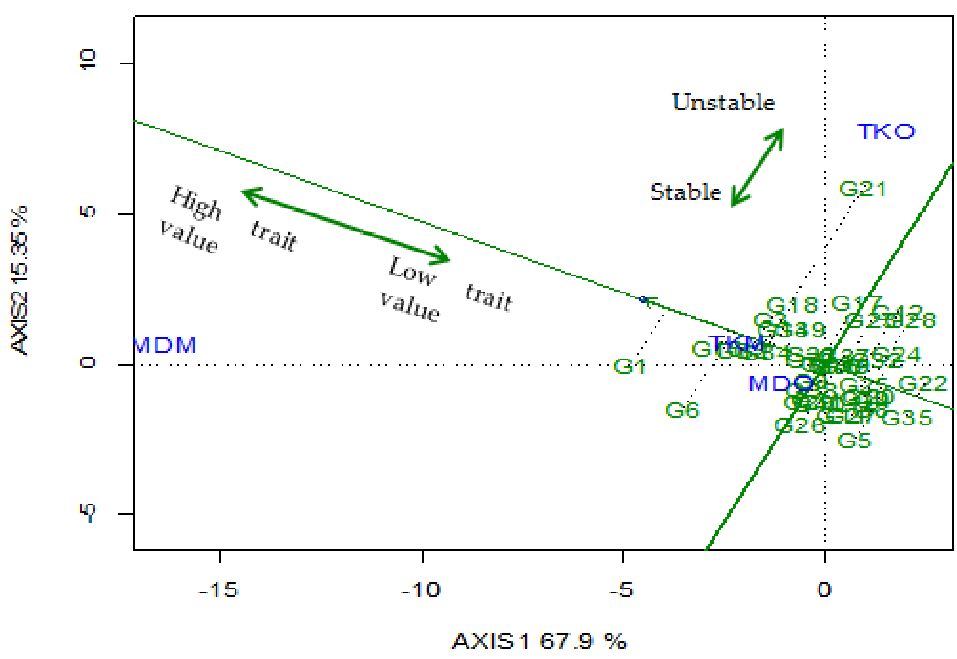
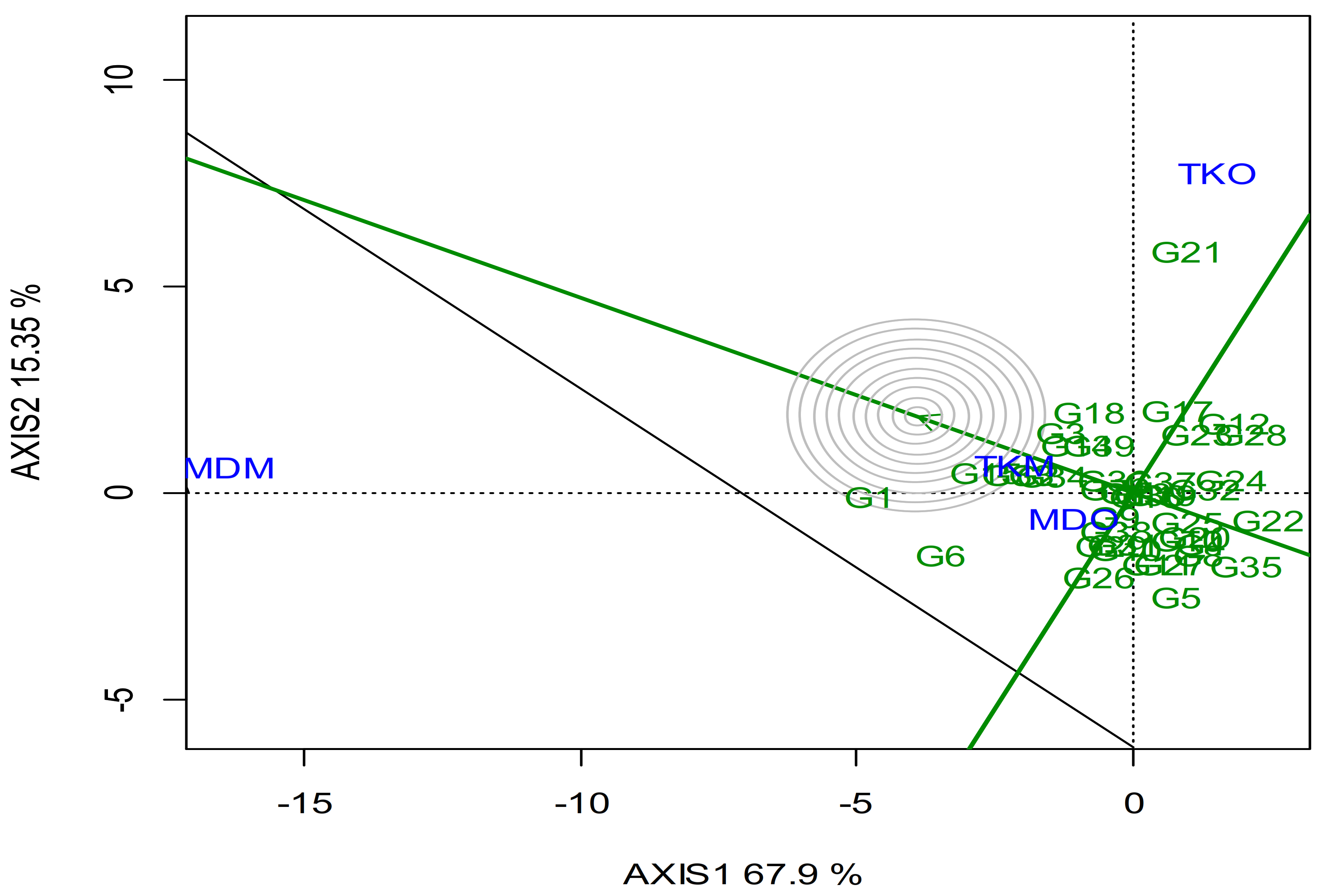
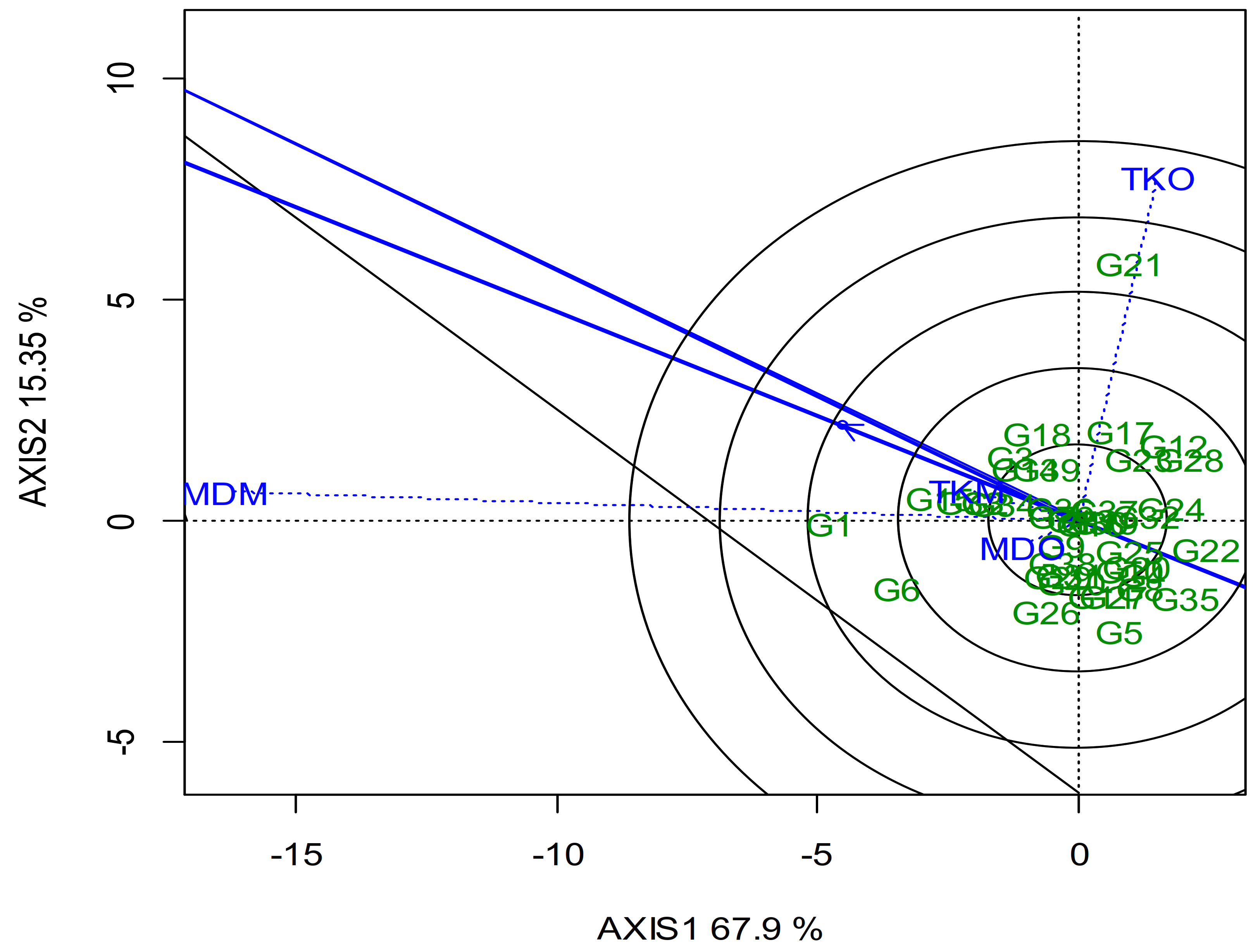
The average-environment coordination (AEC) or average-environment axis (AEA) view of the GGE biplot is used for genotype ranking based on average means performance and their stabilities (Figure 2). This graph is comprised of two lines, the AEC abscissa (vertical line) and the AEC ordinate (horizontal line). The AEC abscissa is the single arrowed line that passes through the hypothetical average environment and through the biplot origin defined by the average scores of PC1 and PC2 of all environments, denoted by the small circle at the tip of the arrowhead (Figure 2). The arrowhead direction on the AEA abscissa points towards higher mean values for yield performances. In this study, the highest and lowest yield per hectare was obtained in G1 and G32, respectively. The second line in the figure measures stability. The line, which is the AEC ordinate, perpendicular to the AEC abscissa that passes through the biplot center, signifies the genotypes’ stability. Genotype vectors farther from the AEC denote higher variability or instability in either direction. Hence, the shorter the distance or projection from AEA, the less variable or more stable the genotype performance among the tested environments, and vice versa. Therefore, G15 is the most stable genotype while G21 is the most unstable among the tested genotypes, (Figure 2). For an extensive selection, the ideal genotypes should typically have both high mean and stability. In this biplot, genotypes G1, G6, and G15 can be described as ideal due to relatively short vectors which are nearer to the AEC. Another reason for the idealness of the AEC is its proximity to the small circle. Generally, yield in the genotypes located on the left side of the line is less than the average mean, whereas genotypes positioned on the right side performed better than the average mean. The genotype with the highest yielding performance but low stability is G1, whereas G15, which was highly stable, had a low yield. The assessment for yield performance is primarily founded on two concepts which are mean and stability; thus, breeders utilize the information obtain from performance assessment to choose genotypes with optimal adaptation to particular environments [13]. Genotype G1 had the highest yielding performance in environment MDM, G6 was highly adapted to TKM, while G21 was best suited to TKO. Figure 3 presents the ranking of genotypes relative to an ideal genotype view with concentric circles. The ideal genotype (i.e., high mean and the most stable) is used as a standard for genotype assessment [23]. Therefore, concentric circles were drawn where the ideal genotype was theoretically located at the center to help visualize the distance between the ideal genotype and each genotype. Since no genotype marker falls within the center of the concentric circle, genotype markers that fall next to the innermost circles are then considered. Thus, G1 and G15 can be considered ideal genotypes for yield per hectare.

3.2.3. Discriminative vs. Representative View of GGE Biplot (Relationship among Test Environments)

The most essential breeding strategy for the effective selection of superior genotypes is the identification of ideal test sites. Representativeness and discriminative power of all environments are the two characteristics of an ideal test environment [21]. The discriminative power of an environment or location refers to its ability to differentiate genotypes while the representativeness refers to the ability of a tested environment to represent other tested environments [21]. In this study, Figure 4 shows the representativeness view vs. discriminative power of the GGE biplot analysis. The cosine of the angle between the average-environment axis and environment vector approximates the correlation coefficient between the genotype means across the environment and the genotype values in that environment [17]. Because the average-environment coordinate (AEC) abscissa is the average-environment axis (AEA), test environments that form small angles with the AEA can better represent the environments compared to those forming large angles. The small circle represents the mean of the environment while the arrow adjacent to the circle signifies the direction of the AEA. The length of the vector estimates the standard deviation (the discriminating ability) of the studied environment. The vector length of a study location provides a measurement of its magnitude (discriminating power) to differentiate genotypes in the environments. Following the above, the short vector locations such as TKM and MDO for yield per hectare can be considered as independent research locations and may be treated as unique locations. Meanwhile, locations with long vectors i.e., MDM and TKO were more influential in discriminating among the rice accessions. Environments having long vectors and small angles with the AEC abscissa are ideal in the selection of superior genotypes. Environment MDM had a long vector and formed a relatively small angle with the AEC abscissa; thus, it was the most representative and discriminating test location. Based on the representativeness and discriminating ability of the study environment, Yan et al. [17] classified the environment into three major types. Type 1 environments are characterized by short vectors, providing little or no information on the genotypes; thus, they are inappropriate as test environments. Type 2 environments are characterized by long vectors, forming smaller angles with the AEC abscissa, and are useful for selecting superior genotypes. Type 3 environments with long vectors form large angles with the AEC abscissa; therefore, they are inappropriate for the selection of superior genotypes. Despite their limitation, Type 3 environments can be useful in culling unstable genotypes. According to this classification, TKM and MDO for yield per hectare were Type 1 environments (short vectors). They offered little or no information on the genotypes and are inappropriate for use as test environments. This implies that some of these environments were redundant and may not be utilized to save the costs of field trials without loss of information. The GGE biplot identified environment MDM for yield per hectare as the ideal environments (Type 2 environments). The environment would be suitable for selecting superior genotypes due to their remarkable discriminating ability and representativeness. Type 3 environments include TKO for yield per hectare, which should not be used in selecting superior genotypes; however, they may be valuable in identifying unstable genotypes. In general, Figure 5 revealed that environment MDM is the ideal environment. This study implies that the type of genotype studied determined the most appropriate location for multilocation assessment based on the test locations’ discriminating power and representativeness.

3.3. Genotype Means Comparison

Grain yield in rice fluctuates significantly with respect to changes in environmental conditions. Therefore, a genotype with a high yield and reasonable stability is desired to develop a new variety to minimize the risk of yield losses in harsh environments and unfavorable low land conditions. In this study, genotype × environment interaction was partitioned, which revealed highly significant differences for genotypes by locations by seasons interaction. These differences are essential in determining GEI. The pooled means across the 4 environments are presented in Table 3. Genotypes G1, G22, and G39 recorded the highest yield at 6.89, 6.03, and 6.16 tons per hectares, respectively, while genotypes G40, G18, and G34 are the bottom-yielding genotypes (Table 3). Yield in rice is a complex trait that is determined by the contribution from yield components traits such as filled grains per panicle, number of effective tillers, and yield per hill/plant [10]. To better comprehend GEI, Becker, and Leon [20] established that genotype evaluation for stability across different seasons and locations could increase both repeatability and heritability of studied traits. Similarly, the significance of GEI indicated changes in genotype ranking or genotype expression across different locations due to the reaction to changes in environmental conditions. Hence, the results from trials conducted in Malaysia indicated that genetic factors control grain yield; however, it is subject to the effect of environmental conditions.

3.4. Univariate Stability Methods

Higher linear component value than non-linear value suggested the probability of prediction for yield performance over the environments. Hence, linear regression coefficient (bi) and non-linear deviation from regression (S2d) of G × E interactions were considered for phenotypic stability analysis [25,26]. According to Eberhart and Russell [25], a stable genotype across a wide range of environments will be one with a high mean and bi of genotypes approximating unity (bi = 1). When the bi is associated with low mean, then the genotypes are described as poorly adapted to all environments. A bi value greater than unity describes a genotype with higher sensitivity to environmental changes and greater adaptation to specific high-yielding environments. In this study, the bi ranged from −0.51 to 2.80. Genotype G16 is considered the most stable due to a bi value closer to unity, followed by G10. Contrarily, genotype G17 was considered the lowest in rank (Table 3). Eberhart and Russell [25] emphasized the use of deviation from regression as a measure of stability, whereas linear regression could be treated as a measure of varietal response to environments. Based on deviation from the regression (S2d) model, a genotype is considered to be stable when S2d is as small as possible (i.e., S2d = 0). Genotype G12 is the most stable, followed by G18, G5, and G27, while G28 followed by G17 are highly unstable genotypes (Table 3).
According to Shukla [27] and Wricke [28], a genotype with low W2i and σi2 is considered stable. Shukla’s stability variance (σi2) is strictly a measure of stability, rather than performance while Wricke’s ecovalence (W2i) defines the contribution of each genotype to the G × E interaction sum of squares. According to these two concepts, genotypes with the smallest stability variance are considered the most stable. In this study, the genotype with the least stability variance σi2 and W2i is ranked highest and considered the most stable. Genotype G5 is considered stable based on σi2 and W2i concepts followed by G23 and 12, while G1 is considered highly unstable, followed by G14 and G28 (Table 3). According to Becker and Leon [20], the range of variables indicates the level of interaction in response to genotypes across environments. Genotypes with the lowest interaction variance are less responsive to the environment, while larger variances indicate environmental influences. However, it was very difficult to find the same pattern of response to validate this proposition, thus, making selection difficult when considering different stability analyses on genotypes due to a shift in genotype ranking. Although different stability parameters are indicative of low, intermediate, or high stability, the stability statistics alone are not useful and informative in genotype selection except if integrated with yield performances. Hence, efforts have been made to combine stability parameters with yield performance in a single selection criterion [19]. Kang [29] developed a yield-stability statistic (YSi) as selection criteria once the G × E interaction is significant and demonstrates the significance of emphasizing stability performance for yield selection. Hence, genotypes with a YSi value greater than the mean are considered stable. Based on this concept, all the evaluated genotypes show relatively stable performance except for G12, G18, G29, G34, and G40 (Table 3).

3.5. Rank Correlations among the Univariate Stability Models

Spearman’s correlation was conducted between the genotype means and the stability parameters that produce stability ranking, as presented in Table 4. The univariate stability parameter measure includes corrected means by least squares (M), regression coefficient (bi), deviation from regression (S2d), Wricke’s ecovalence (W2i), Shukla’s stability variance (σi2), and Kang’s stability statistic (YSi). The analysis was used for the identification of agreement among the stability parameters. In this study, YSi was positively and highly significantly correlated with mean, while a negative and highly significant correlation with mean was recorded for all other parameters except for bi where the non-significant correlation was observed (Table 4). Mekbib [30] reported that statistical stability parameters provide information that cannot be quantified from the trait’s means. The stability ranking given by the stability parameters of S2d was highly correlated with σi2 and W2i at 0.83. This indicates an agreement in the ranking of stability from one method to the other for the genotypes. These two stability parameters reflect only the genotypes’ response to the environment and the G × E interaction, but not the genotypes’ performance themselves. However, a non-significant correlation was observed between bi and other stability parameters.

4. Conclusions

Yield is a complex trait that is highly influenced by the environment. Hence, plant breeders test newly developed lines across the environment before commercialization or release as a variety. Joint regression analysis is the most widely used stability analysis for interpretation of GEI; however, it has several limitations. Recently, GGE biplot has overcome the limitations of Joint regression analysis. This study evaluated the stability of grain yield of advanced fragrant rice genotype derived from crosses between MR219 and Basmati 370 using different stability models and found that the results of both multivariate and univariate statistical analyses were in agreement. Similarly, each statistical model was able to discriminate the main differences in genotypes stability, and results established G × E interaction with yield performance across different environments. Based on average ranking generated from measuring multivariate and univariate stability, rice accessions were classified into three main categories, viz., genotypes having high trait performance, and high stability (G1) as category 1. The second category consists of genotypes that exhibited high mean performance but low stability (G6), while the third category includes genotypes with high stability but low trait performance (G15). Our results showed that breeding for yield performance was possible, and the identified genotypes could be recommended for commercial cultivation.

Author Contributions

Conceptualization, M.Y.R. and N.H.; methodology, N.H. and M.Y.R.; software, Y.O.; formal analysis, N.H., M.Y.R. and Y.O.; resources, A.R.; writing—original draft preparation, N.H., M.Y.R. and Y.O.; writing—review and editing, M.R.I., A.R., F.A. and S.C.; All authors offered suggestions on various drafts of the manuscript. All authors have read and agreed to the published version of the manuscript.

Funding

This research was funded by the Ministry of Education Malaysia, Higher Institution Centers of Excellence (HICoE), grant number 6369105.

Institutional Review Board Statement

Not applicable.

Informed Consent Statement

Not applicable.

Data Availability Statement

All data supporting this finding are presented in tables and figure embedded within the manuscript.

Conflicts of Interest

The authors declare no conflict of interest.

References

  1. Oladosu, Y.; Rafii, M.Y.; Abdullah, N.; Abdul Malek, M.; Rahim, H.A.; Hussin, G.; Kareem, I. Genetic variability and selection criteria in rice mutant lines as revealed by quantitative traits. Sci. World J. 2014. [Google Scholar] [CrossRef] [PubMed] [Green Version]
  2. Asma, I.K.; Rafii, M.Y.; Sobri, H.; Anna, L.P.K.; Rahim, A.H.; Mahmud, T.M.M.; Oladosu, Y. Physicochemical characteristics and nutritional compositions of MR219 mutant rice and their effects on glycaemic responses in BALB/c mice. Int. Food Res. J. 2019, 126, 1477–1484. [Google Scholar]
  3. Oladosu, Y.; Rafii, M.Y.; Samuel, C.; Fatai, A.; Magaji, U.; Kareem, I.; Kolapo, K. Drought resistance in rice from conventional to molecular breeding: A review. Int. J. Mol. Sci. 2019, 20, 3519. [Google Scholar] [CrossRef] [PubMed] [Green Version]
  4. Oladosu, Y.; Rafii, M.Y.; Arolu, F.; Chukwu, S.C.; Muhammad, I.; Kareem, I.; Arolu, I.W. Submergence tolerance in rice: Review of mechanism, breeding and future prospects. Sustainability 2020, 12, 1632. [Google Scholar] [CrossRef] [Green Version]
  5. Giraud, G. The world market of fragrant rice, main issues and perspectives. Int. Food Agribus. Manag. Rev. 2013, 16, 1–20. [Google Scholar]
  6. Singh, R.K.; Gautam, P.L.; Saxena, S.; Singh, S. Scented Rice Germplasm: Conservation, Evaluation and Utilization. In Aromatic Rices; Singh, R.K., Singh, U.S., Khush, G.S., Eds.; Oxford & IBH: Kalyani, New Delhi, 2000; pp. 107–133. [Google Scholar]
  7. Lau, W.C.P.; Rafii, M.Y.; Ismail, M.R.; Puteh, A.; Latif, M.A.; Asfaliza, R.; Miah, G. Development of advanced fragrant rice lines from MR269× Basmati 370 through marker-assisted backcrossing. Euphytica 2017, 213, 1–15. [Google Scholar] [CrossRef]
  8. Oladosu, Y.; Rafii, M.Y.; Abdullah, N.; Magaji, U.; Miah, G.; Hussin, G.; Ramli, A. Genotype× Environment interaction and stability analyses of yield and yield components of established and mutant rice genotypes tested in multiple locations in Malaysia. Acta Agric. Scand B Soil Plant Sci. 2017, 67, 590–606. [Google Scholar] [CrossRef]
  9. Sabri, R.S.; Rafii, M.Y.; Ismail, M.R.; Yusuff, O.; Chukwu, S.C.; Hasan, N.A. Assessment of agro-morphologic performance, genetic parameters and clustering pattern of newly developed blast resistant rice lines tested in four environments. Agronomy 2020, 10, 1098. [Google Scholar] [CrossRef]
  10. Oladosu, Y.; Rafii, M.Y.; Magaji, U.; Abdullah, N.; Miah, G.; Chukwu, S.C.; Kareem, I. Genotypic and phenotypic relationship among yield components in rice under tropical conditions. Biomed. Res. Int. 2018. [Google Scholar] [CrossRef] [Green Version]
  11. Myint, K.A.; Amiruddin, M.D.; Rafii, M.Y.; Abd Samad, M.Y.; Ramlee, S.I.; Yaakub, Z.; Oladosu, Y. Genetic diversity and selection criteria of MPOB-Senegal oil palm (Elaeis guineensis Jacq.) germplasm by quantitative traits. Ind. Crops Prod. 2019, 139, 111558. [Google Scholar] [CrossRef]
  12. Wade, L.J.; McLaren, C.G.; Quintana, L.; Harnpichitvitaya, D.; Rajatasereekul, S.; Sarawgi, A.K.; Sarkarung, S. Genotype by environment interactions across diverse rainfed lowland rice environments. Field Crops Res. 1999, 64, 35–50. [Google Scholar] [CrossRef]
  13. Yan, W.; Hunt, L.A.; Sheng, Q.; Szlavnics, Z. Cultivar evaluation and mega-environment investigation based on the GGE biplot. Crop. Sci. 2000, 40, 597–605. [Google Scholar] [CrossRef]
  14. Redona, D.E. Standard Evaluation System (SES) for Rice, 5th ed.; International Rice Research Institute: Los Baños, CA, USA, 2013. [Google Scholar]
  15. Dia, M.; Wehner, T.C.; Arellano, C. Analysis of Genotype X Environment Interaction (GxE) Using SAS Programming. 2015. Available online: http://cuke.hort.ncsu.edu/cucurbit/wehner/software.html (accessed on 17 February 2021).
  16. RStudio. RStudio: Integrated Development Environment for R (Computer Software v0.98.1074). 2014. Available online: http://www.rstudio.org/ (accessed on 17 February 2021).
  17. Yan, W.; Kang, M.S.; Ma, B.; Woods, S.; Cornelius, P.L. GGE biplot vs. AMMI analysis of genotype-by-environment data. Crop. Sci. 2007, 47, 643–653. [Google Scholar] [CrossRef]
  18. Dehghani, H.; Ebadi, A.; Yousefi, A. Biplot analysis of genotype by environment interaction for barley yield in Iran. Agron J. 2006, 98, 388–393. [Google Scholar] [CrossRef]
  19. Kang, M.S.; Pham, H.N. Simultaneous selection for high yielding and stable crop genotypes. Agron J. 1991, 83, 161–165. [Google Scholar] [CrossRef]
  20. Becker, H.C.; Leon, J. Stability analysis in plant breeding. Plant. Breed. 1988, 101, 1–23. [Google Scholar] [CrossRef]
  21. Oladosu, Y.; Rafii, M.Y.; Magaji, U.; Abdullah, N.; Ramli, A.; Hussin, G. Assessing the representative and discriminative ability of test environments for rice breeding in Malaysia using GGE Biplot. Int. J. Sci. Technol. Res. 2017, 6, 8–16. [Google Scholar]
  22. Haldane, J.B.S. The interaction of nature and nurture. Ann. Eugen. 1946, 13, 197–205. [Google Scholar] [CrossRef]
  23. Yan, W.; Kang, M.S. GGE Biplot Analysis: A Graphical Tool for Breeders, Geneticists, and Agronomists; CRC Press: New York, NY, USA, 2002; p. 71. [Google Scholar]
  24. Gauch, H.G.; Zobel, R.W. AMMI Analysis of Yield Trials. In Genotype by Environment Interaction; Kang, M.S., Gauch, H.G., Eds.; CRC Press: Boca Raton, FL, USA, 1996; pp. 85–122. [Google Scholar]
  25. Eberhart, S.T.; Russell, W.A. Stability parameters for comparing varieties 1. Crop. Sci. 1966, 6, 36–40. [Google Scholar] [CrossRef] [Green Version]
  26. Finlay, K.W.; Wilkinson, G.N. The analysis of adaptation in a plant-breeding programme. Aust. J. Agric. Res. 1963, 14, 742–754. [Google Scholar] [CrossRef] [Green Version]
  27. Shukla, G.K. Some statistical aspects of partitioning genotype environmental components of variability. Heredity 1972, 29, 237–245. [Google Scholar] [CrossRef]
  28. Wricke, G. Uber eine Methode zur Erfassung der okologischen Streubreite in Feldverzuchen. Z. Pflanzenzuchtg 1962, 47, 92–96. [Google Scholar]
  29. Kang, M.S. Simultaneous selection for yield and stability in crop performance trials: Consequences for growers. Agron. J. 1993, 85, 754–757. [Google Scholar] [CrossRef]
  30. Mekbib, F. Yield stability in common bean (Phaseolus vulgaris L.) genotypes. Euphytica 2003, 130, 147–153. [Google Scholar] [CrossRef]
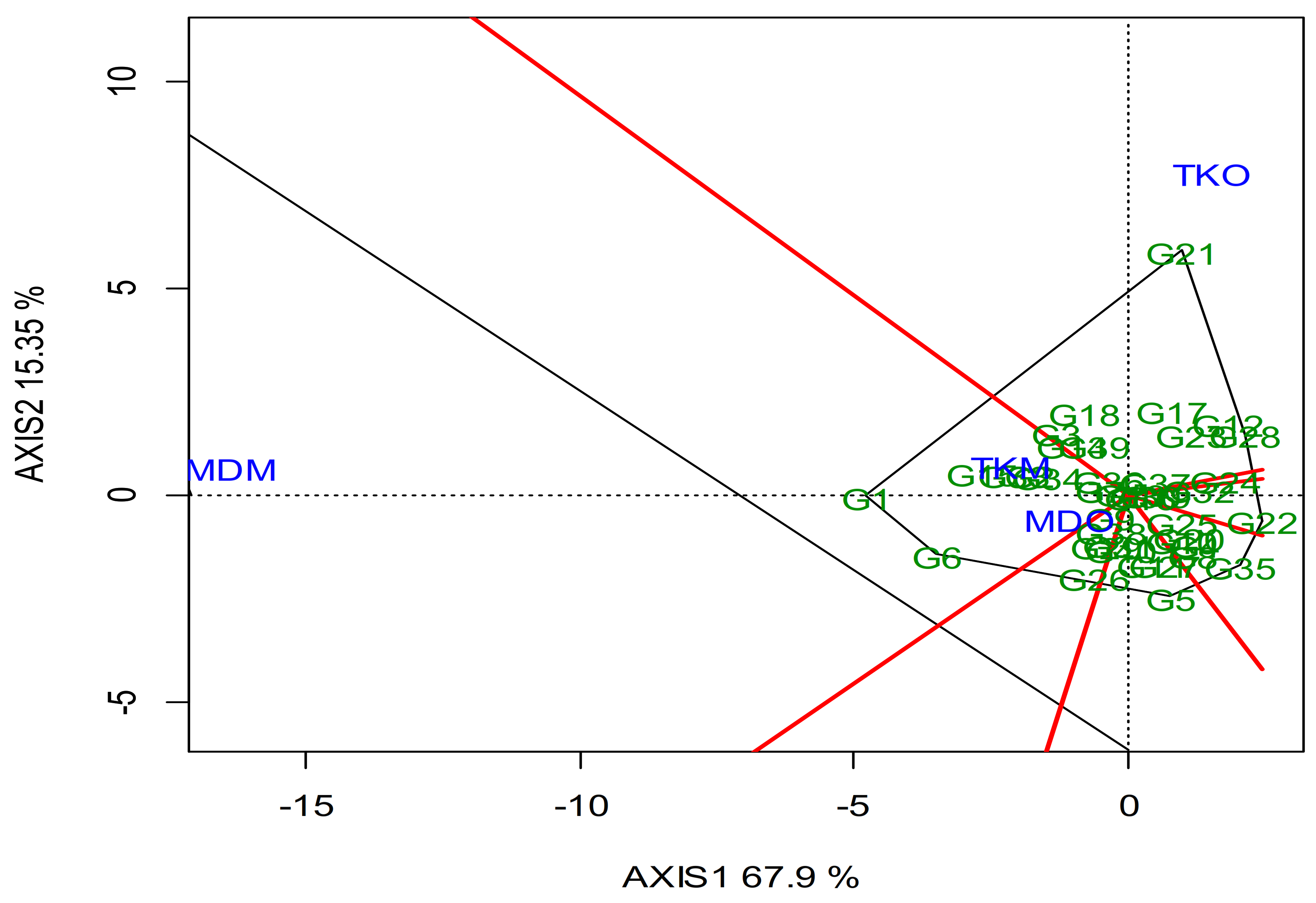
Figure 1. The polygon view showing the which-won-where pattern of genotype main effects plus genotypic × environment interaction effect biplot for yield per hectare of 40 rice accessions tested in 4 environments. The biplots were based on SVP = 2, Centering = 0, and Scaling = 0. The key to the accession labels is G1-G38 = line 1–38, G39 = MR219, G40 = B370, and the environment is shown in Table 1.
Sustainability 13 04555 g001
Figure 2. The mean vs. stability view showing the genotype main effects plus genotypic × environment interaction effect biplot (G + G × E) interaction effect of 40 rice genotypes in 2 seasons and 2 locations for yield per hectare of 40 rice accessions tested in 4 environments.
Sustainability 13 04555 g002
Figure 3. The genotypes comparison with ideal genotype view showing genotype main effects plus genotypic × environment interaction effect biplot (G + G × E) interaction effect of 40 rice genotypes in 2 seasons and 2 locations for yield per hectare of 40 rice accessions tested in 4 environments.
Sustainability 13 04555 g003
Figure 4. Discrimitiveness vs. representativeness of environment view showing genotype main effects plus genotypic × environment interaction effect biplot (G + G × E) interaction effect of 40 rice genotypes in 2 seasons and 2 locations for yield per hectare of 40 rice accessions tested in 4 environments.
Sustainability 13 04555 g004
Figure 5. Environment ranking view showing genotype main effects plus genotypic × environment interaction effect biplot (G + G × E) interaction effect of 40 rice genotypes in 2 seasons and 2 locations for yield per hectare of 40 rice accessions tested in 4 environments.
Sustainability 13 04555 g005
Table 1. Characterization and description environment.
Location CodeSeasonCoordinateSoil TextureAlt.Av. Temp.Av. HumAv. Rainfall (Monthly)
TKMMain3°25′0″ N 101°10′ ESilty clay loam3 m23 °C–31 °C83792.6 (197.6)
MDOoff5°59′ N 100°24′ EClay loam18 m25 °C–38 °C63487.7 (122.7)
MDMMain5°59′ N 100°24′ EClay loam18 m22 °C–33 °C91560.6 (138.2)
TKOoff3°25′0″ N 101°10′ ESilty clay loam3 m25 °C–37 °C65489.5 (120.7)
Note: TKM: Tanjung Karang main season; TKO: Tanjung Karang off season; MDM: Kedah main season; MDO: Kedah off season.; Alt.: altitude; Av. Temp.: average temperature; Av. Hum.: average humidity; main season: August–February; off season: March–July.
Table 2. Analysis of variance for grain yield per hectare among 40 rice genotypes grown in 4 environments.
SourceDFMean Square% of GE
Rep (location)418.86 **2.00
Location (L)1578.69 **37.01
Season (S)1237.64 **6.31
Genotype (G)398.81 **15.36
G × S398.85 **9.16
G × L398.01 **8.29
G × L × S4011.99 **12.73
Error3164.419.12
Note: DF: degree of freedom, ** highly significant at p ≤ 0.01.
Table 3. Means (corrected by least squares) (M), regression coefficient (bi), deviation from regression (S2d), Wricke’s ecovalence (W2i), Shukla’s stability variance (σi2), and Kang’s stability statistic (YSi) for yield per hectare among 40 rice genotypes tested in four locations.
GenMEANbiS2dW2iσi2YSi
G16.89 ± 1.58 a0.7010.90154.7054.08 ***34
G24.68 ± 0.53 b–j2.328.62 *42.3614.67 *15
G34.36 ± 0.61 c–k0.522.7215.985.4116
G45.28 ± 0.92 a–i1.213.3918.576.3231
G55.07 ± 0.83 b–j−0.200.350.590.0129
G64.29 ± 0.71 d–k1.440.812.390.6415
G75.06 ± 0.77 b–j1.382.065.671.7928
G85.70 ± 0.79 a–f1.980.972.480.6736
G94.17 ± 0.72 e–k0.651.354.541.3910
G105.27 ± 0.97 a–i1.154.1232.1911.09 *26
G115.44 ± 0.95 a–h0.013.8817.145.8232
G123.39 ± 0.57 jk1.310.292.040.521
G134.03 ± 0.60 f–k0.607.45 *21.257.268
G145.88 ± 1.50 a–d2.288.86103.0235.95 ***30
G155.02 ± 0.64 b–j0.061.923.050.8727
G164.27 ± 0.45 d–k0.934.1920.957.1514
G175.47 ± 1.21 a–h2.8011.6734.3311.85*29
G183.73 ± 0.47 ijk1.380.332.070.533
G194.18 ± 0.92 e–k0.222.304.271.3011
G204.91 ± 0.85 b–j1.669.5217.706.0126
G215.48 ± 0.80 a–h0.423.829.783.2334
G226.03 ± 1.19 abc1.682.7361.1321.25 **31
G234.46 ± 0.62 c–j−0.041.130.650.0318
G244.68 ± 0.53 b–j0.493.1415.345.1920
G255.81 ± 0.90 a–e2.272.006.962.2437
G264.24 ± 0.73 d–k2.342.072.380.6412
G273.84 ± 0.50 h–k1.370.354.591.415
G285.56 ± 1.23 a–g0.0521.4773.4625.58 ***27
G293.83 ± 0.53 h–k−0.044.8753.8818.71 **−4
G303.87 ± 0.41 h–k0.771.6020.887.136
G314.25 ± 0.45 d–k−0.51 *2.449.943.2913
G324.89 ± 0.89 b–j2.185.4117.145.8225
G333.91 ± 0.59 g–k1.570.772.420.657
G343.73 ± 0.47 ijk0.813.4836.6012.64 *−2
G354.84 ± 0.77 b–j0.452.046.762.1724
G364.82 ± 0.51 b–j1.270.743.421.0023
G374.39 ± 0.70 c–j0.751.114.601.4217
G384.16 ± 0.47 e–k1.202.1912.514.199
G396.16 ± 0.92 ab0.411.4820.036.8340
G402.70 ± 0.30 k0.180.377.672.49−1
* Significance level at 0.05 level of probability; ** Significance level at 0.01 level of probability; *** Significance level at 0.001 level of probability. least significant difference (LSD) (4.22). Genotype means having the same letter are not significantly different at 5% probability level.
Table 4. Spearman rank correlations among univariate stability parameters and trait mean (M) for 40 rice genotypes tested in 4 locations.
MbiS2dW2iσi2YSi
M1
bi01
S2d−0.40 **0.041
W2i−0.33 *0.130.83 ***1
σi2−0.33 *0.130.83 ***1.00 ***1
YSi0.98 ***−0.03−0.29−0.19−0.191
Note: Mean: M, regression coefficient: bi, deviation from regression: S2d, Wricke’s ecovalence: W2i, Shukla’s stability variance: σi2, Kang’s stability statistic: YSi, *** Significance level at 0.001; ** Significance level at 0.01; * Significance level at 0.05 level of probability.
Publisher’s Note: MDPI stays neutral with regard to jurisdictional claims in published maps and institutional affiliations.