Local Drivers Associated to Temporal Spectral Response of Chlorophyll-a in Mangrove Leaves

Abstract

The pigment content in leaves has commonly been used to characterize vegetation condition. However, few studies have assessed temporal changes of local biotic and abiotic factors on leaf pigments. Here, we evaluated the effect of local environmental variables and tree structural characteristics, in the chlorophyll-a leaf concentration (Chl-a) associated with temporal change in two mangrove species. Rhizophora mangle (R. mangle) and Avicennia germinans (A. germinans) trees of a fringe mangrove forest (FMF) and lower basin mangrove forest (BMF) were visited over a period of one year, to obtain radiometric readings at leaf level to estimate Chl-a. Measurements on tree characteristics included diameter at breast height (DBH), basal area (BA), and maximum height (H). Environmental variables included soil interstitial water temperature (T_i), salinity (S_i), and dissolved oxygen (O_i), flood level (fL), ambient temperature (T_amb), and relative humidity (H_rel). Generalized linear models and covariance analysis showed that the variation of Chl-a is mainly influenced by the species, the interaction between species and mangrove forest type, DBH, seasonality and its influence on the species, soil conditions, and fL. Studies to assess spatial and temporal change on mangrove forests using the spectral characteristics of the trees should also consider the temporal variation of leave chlorophyll-a concentration.

1. Introduction

Mangrove forests (MFs) are of great ecological and economic importance to humans, especially from coastal communities [1]; they are highly productive [2,3,4], generate large amounts of nutrients and organic matter that subsequently contributes to soil formation and coastal erosion control [5,6], they are ecosystems that provide food, shelter and breeding to a wide variety of flora and fauna including commercial species, and they are key to reductions in the greenhouse gases (GHG) effect. The conditions of the floodable soil of MFs allow GHG to be purified and hijacked in the soil by biogeochemical processes, degradating organic matter which is then incorporated into the soil [7,8].

The distribution and presence of mangroves depends on the geomorphological and ecological characteristics of the region, which are influenced by the average sea level, climate, and hydrology [9,10,11,12]. The hydrology, for example, contributes to the transport, deposition, and accumulation or erosion of sediments, and determines the oxidation–reduction conditions in the soil. One important characteristic of the t hydrology is the hydroperiod, which is affected by fluctuations in the groundwater level, tides, terrestrial runoff, and precipitations. A floodable soil promotes physical and chemical conditions that influence soil anaerobiosis, the accumulation of organic matter in sediments, and the availability of salts, nutrients, and oxygen [13].

Most of the studies that assess environmental effects on mangroves consider regional scales. However, local characteristics such as the soil type, hydroperiod and climate are combined to expose MFs to hydric and saline stress that directly affects the productivity of their biomass [14,15]. Biomass in MFs is composed of the biomass of the aerial and underground components. Underground biomass depends on the aerial biomass that falls and incorporates into the soil by biogeochemical processes. Aerial biomass depends on the photosynthetic capacity of the leaf that determines its growth and physiology [16] and may be compromised by the hydric and saline stress of the soil.

During prolonged periods of light and hydric stress, the photosynthetic activity of the leaf and the opening of the stoma decreases because of the reduction in the availability of reaction centers [17]. On the contrary, precipitation directly affect the concentration of Chl-a in leaves, increasing significantly during the rainy season [18,19].

In MFs, it is common to find soils with hypersaline conditions, marked hydrological changes, and climatic temporalities with high irradiation. However, the optimal growth of the mangrove species occurs in areas that receive at least 50% of solar attenuation. A higher frequency of light saturation and an excess of light is more likely to lead to photoinhibition and other harmful effects on the leaf [20]. Therefore, the concentration of photosynthetic pigments in the leaf is related to the physiological stress determined by the availability of water, the interstitial salinity, flooding periods, the variation in the incidence of solar irradiance, the climate influence, and humidity, influencing the growth of the leaf at the same time [21,22].

In the leaf, light energy is absorbed by antenna biomolecules called pigments that capture light and transfer it to the reaction center [23]. The pigment contained in the leaf varies according to the amount of solar radiation absorbed. Low concentrations of pigments in the leaf directly limit the photosynthetic activity, and at the same time, the photosynthetic production [24,25,26,27]. Associated photosynthetic pigments include the decomposition compounds of chlorophyll (Chl), chlorophyll-a and chlorophyll-b (its derivatives), carotenoids, and xanthophylls [28].

Chl is organized into light-capturing structures, called antenna complexes, attached to proteins. The photosystems I and II convert light energy into chemical energy through a reaction center. Chemical energy is stored in high caloric power compounds that give the leaf the green color, which is related to the leaf’s ability to absorb the red and blue fractions of sunlight [29,30].

The spectral response of the photosynthetically active region of the leaf is characterized by a low reflectance in the visible region due to the strong absorption by photosynthetic pigments, mainly carotenes and chlorophyll-a in a range of 504 nm to 680 nm, with a high reflectance in the near-infrared (NIR) region that relates to leaf morphology [31]. Chlorophyll-a is the photosynthetic pigment in the leaf that is responsible for light energy fixation into leaf components (e.g., starch, cellulose, nitrogen) [31,32,33]. This pigment is associated with reflectance values in the visible region of the electromagnetic spectrum [34], the NIR [35] (in the 520 nm, 560 nm, 650 nm, 710 nm, 760 nm, 2100 nm and 2230 nm bands), and the red band (from 739 nm to 742 nm) [33]. Reflectance in the bands 739 nm and 742 nm relates to the leaf health condition and stress [36].

There is a large amount of literature related to pigment content in mangrove leaves. However, few studies have evaluated the effect of local environmental variables and tree structural variables and forest characteristics on the temporal variation of Chl-a at the leaf level. The objective of this work is to determine the structural characteristics at the tree-level of the two species present in two types of MF, their temporal changes, and their relationship to local environmental variables that influence the concentration of Chl-a at the leaf level. This was addressed through exploring the temporal relationship of Chl-a leaf concentration of R. mangle and A. germinans with the ambient temperature (T_amb), relative humidity (H_rel), flood level (fL), soil interstitial water salinity (S_i), temperature (T_i), and dissolved oxygen (O_i), tree height (H), diameter at breast height (DBH) and basal area (BA) in mangrove forests of a lagoon fringe and basin types of a karst region.

2. Materials and Methods

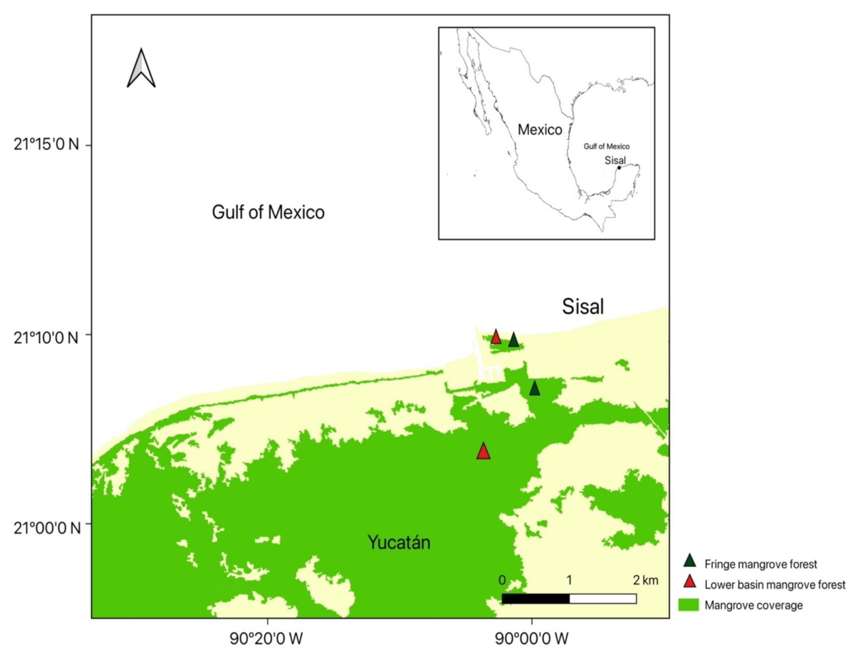
2.1. Study Area

Mexico has the fourth largest mangrove area in the world, with 905,086 hectares, of which 60.12% correspond to the coastal shoreline of the karst region of the Yucatán Peninsula (PY)), with the presence of R. mangle, A. germinans and L. racemosa in different mangrove configurations [37]. Sisal Seaport (Figure 1) is located in the municipality of Hunucma, Yucatan, Mexico. It is delimited to the north by the Gulf of Mexico, and it is part of the protected area “Reserva Estatal Cienagas y Manglares de la Costa Norte de Yucatán”. The karst soil (K_s) in PY is formed of highly soluble carbonated rocks that allow the formation of dolines and terrestrial filtrations to the underlying aquifers which, during the rainy season, are recharged and saturate the flooding soil in some areas near the coast [38].

Two MFs were selected, both with the presence of R. mangle and A. germinans. The fringe mangrove forest (FMF) presents soil lacking organic matter of the karst limestone type formed by fine and medium sands, with some deposits of shell. The irregularities in the topography of the FMF terrain have led to the formation of a shallow depression that allows the stagnation of water from rain and local temporal water discharges. R. mangle trees are present on the lagoon fringe followed by A. germinans trees. The lower basin mangrove forest (BMF) presents clay soil with little organic matter of the Carso-tectonic type of coastal floodplain marsh. R. mangle trees are seen over the least shallow region in combination with A. germinans trees over the shallowest region. It does not have seawater influence and the soil is flooded by rain and a periodic tidal interval of less than 30 cm from springs located further south.

Data collection

Field data were collected every 15 days from September 28, 2016, to September 13, 2017, in an FMF and BMF of Sisal Seaport. According to the methodology described in the collection manual of Mexico’s National Forestry and Soil Inventory [39], at the beginning of each campaign, soil interstitial water samples were extracted for the measurement of physicochemical parameters to avoid altering the environment with the sampling process. Each sample was extracted with a siphon and syringe (60 ml). The siphon was an adaptation of a 30 mm diameter and 50 cm long acrylic tube, perforated at one end connected to a 30 mm diameter plastic hose. Each sample was measured for T_i, S_i and O_i with a YSI Pro 2030 model multiparameter probe.

In each campaign, T_amb and H_rel were recorded with an AMPROBE anemometer TMA40-A model, and the fL was assessed with a fixed graduated stake for the FMF and BMF. In each MF, three R. mangle and A. germinans trees were randomly selected and marked with forest tape to measure the same tree throughout the study. Each tree had its height measured with a HAGLÖF vertex model IV HS102 hypsometer, its DBH with a vernier scale considering the main trunk [40], and the BA using Equation (1) described in the field guide for mangrove identification [41]:

$$BA=\left(r^2\right)\left(\pi \right), where r=\frac{DBH}{2}$$

(1)

For each tree, 15 leaves were randomly selected in the high region of the canopy receiving sunlight directly, and 15 leaves in the middle region of the canopy receiving sunlight indirectly, and their reflectance was measured. A total of 30 radiometric readings per tree were obtained with a portable spectroradiometer (GER 1500 model, Spectra Vista Corp.) equipped with a leaf clip, an integrated calibration panel, and an optical fiber cable. The radiometric readings were calibrated every five readings, obtaining information from 512 bands (350 to 1050 nm) with a 3.2 nm resolution. Readings were averaged per tree. According to the methodology described for the Yucatán Peninsula’s mangroves [33], the radiometric readings were used to calculate the green normalized difference vegetation index (greenNDVI) using Equation (2) [34], where ρNIR and ρGREEN are the average reflectance values in the near-infrared (750 nm) and green (550 nm) wavelengths, respectively:

$$greenNDVI=\frac{\left(\mathsf{\rho }\mathrm{NIR}- \mathsf{\rho }\mathrm{GREEN}\right)}{\left(\mathsf{\rho }\mathrm{NIR}+ \mathsf{\rho }\mathrm{GREEN}\right)}$$

(2)

Subsequently, the value obtained from greenNDVI was used in Equation (3), where “x” corresponds to the value of greenNDVI for the calculation of Chl-a leaf concentration [35]:

$$\mathrm{Chl}-\mathrm{a}= -54.545+149.39\mathrm{x}$$

(3)

2.2. Data Analysis

The assumptions of normality, homogeneity, and independence were not met. Therefore, a generalized linear model (GLM) was applied with a gamma-type error distribution in the dependent variables with a coefficient of constant variation and a logarithmic (log) ligation function [42], using the software R (R Core Team).

A primary model (Mod₀) was established that considered all variables: T_i, S_i, O_i, fL, H_rel, T_amb, DBH, BA, H, MF, species (Spp) and time to explain the variation of Chl-a leaf concentration. A covariance analysis with the “Fisher” test was applied to Mod₀ to determine the amount of variance explained by the model [43], and subsequently the Akaike information criterion (AIC) [43,44], with elimination selection, was used to obtain the most parsimonious model (Mod₁). The AIC eliminated the least influential variable on Chl-a leaf concentration according to the individual contrast by comparing the models with the null hypothesis (H0) “the population means normally distributed with standard deviation and variance are equal”. With the resulting Mod₁, a new covariance analysis with the “Fisher” test was performed to determine the significance level α = 0.05 and the influence of variables on the Chl-a.

3. Results

3.1. Fringe Mangrove Forest

Both species presented reflectance curves typical of vegetation (Figure 2). The Avicennia germinans presented the highest peaks in the 550 nm band.

The FMF environment recorded a T_amb range between 23.2 °C and 38.2 °C in January and October, respectively, with a variation margin of 2.9 °C between dates and an H_rel of 30.1% to 74.8% with a variation of 10.7%. The lowest value of H_rel was recorded in April, and the highest in August. Both T_amb and H_rel values were typical of the region and coincided with weather seasons marked as dry in the months from March to May, rainy from June to October, and north winds from November to February.

The first campaign conducted in September 2016 recorded an fL of 0.47 m, and it was taken as a reference for the following dates. A minimum of 0.23 m and maximums of 0.75 m of fL were recorded throughout the year. Minimum flood levels were observed in May, which corresponded to the dry season, and maximum values related to the rainy season. Dissolved O_i levels of 2.3% to 7.3% were recorded in September during the rainy season, at the beginning and the end of the month, respectively. The lowest T_i recorded was 20.4 °C in January during the north winds season, and the highest was in April with 31.1 °C during the region’s dry season. The S_i in FMF was marine, with values of 19.05 psu in the month of August to 34.6 psu in March. On average, FMF presented an fL of 0.56 m with variations of 0.14 m, a mean of 49.38% of dissolved O_i, and 28.53 of S_i psu.

Both species (

Table 1. Basic tree dasometric variables in the fringe mangrove forest. Tree height (H), diameter at breast height (DBH), basal area (BA), chlorophyll-a leaf concentration (Chl-a), standard deviation (SD), and standard error (SE).

Species	Data	Min	Max	Mean	±SD	±SE
R. mangle	H (m)	2.70	3.30	3.02	0.02	0.01
	DBH (cm)	2.60	4.20	3.44	0.36	0.07
	BA (cm2)	5.31	13.85	9.46	1.93	0.39
	Chl-a (μg per cm−2)	24.83	44.81	34.08	2.66	0.54
A. germinans	H (m)	2.50	3.20	2.81	0.04	0.01
	DBH (cm)	3.10	4.70	3.82	0.21	0.04
	BA (cm2)	7.55	17.35	11.57	1.27	0.26
	Chl-a (μg per cm−2)	4.86	28.60	14.63	4.91	1.00

) presented constant H over time. The R. mangle trees recorded a H from 2.7 to 3.3 m with DBH from 2.6 to 4.2 cm and BA from 5.3 to 13.9 cm². Their leaves recorded Chl-a between 24.83 µg per cm² and 44.81 µg per cm², and an annual average of 34.08 µg per cm² (SD ± 2.66). The A. germinans trees recorded very similar H values, between 2.5 and 3.2 m with a DBH from 3.1 to 4.7 cm, and average BA from 7.5 to 17.3 cm². The Chl-a in their leaves ranged between 4.86 and 28.59 µg per cm², with an annual average of 14.63 µg per cm² (SD ± 4.91). In the FMF, the R. mangle species recorded the highest efficiency for Chl-a production despite recording lower dasometric measurements.

3.2. Lower Basin Mangrove Forest

Both species presented reflectance curves typical of vegetation (Figure 3). The R. mangle of the BMF showed higher peaks at 760 nm. The highest A. germinans peaks were at 550 nm. This was also observed in the FMF.

At the beginning of the sampling period, a 0.44 m fL was observed in the BMF. This flood level was taken as the reference for further measurements. The variation in fL ranged between 0.0 and 1 m, registering the lowest level in the months of May and June and the highest in January. From May to June, the BMF was found to be completely dry, and the lack of water in the soil did not allow the collection of interstitial water samples. Therefore, no records of T_i, S_i or O_i were obtained in those months. The soil interstitial water in BMF showed dissolved O_i levels of up to 4.42% in December, and T_i maximums of 36.1 °C in August. Hypersaline values, S_i of 44.8 psu were observed in September.

On average, the BMF presented an fL of 0.73 m with a variation of 0.3 m between dates, with average O_i and S_i of 23.48% and 22.04 psu, respectively. The T_amb values in the BMF were recorded between 24.7 and 38.8 °C in January and September, respectively, with a minimum H_rel of 42.1% in May and a maximum H_rel of 81.1% in August.

A very similar H (

Table 2. Basic tree dasometric variables in the lower basin mangrove forest. Tree height (H), diameter at breast height (DBH), basal area (BA), chlorophyll-a leaf concentration (Chl-a), standard deviation (SD), and standard error (SE).

Species	Data	Min	Max	Mean	±SD	±SE
R. mangle	H (m)	2.40	3.40	2.93	0.07	0.01
	DBH (cm)	1.90	6.00	3.80	0.18	0.04
	BA (cm2)	2.84	28.27	12.72	0.72	0.15
	Chl-a (μg cm−2)	9.55	36.27	24.35	3.56	0.73
A. germinans	H (m)	2.50	3.30	2.89	0.24	0.05
	DBH (cm)	1.90	3.30	2.57	0.21	0.04
	BA (cm2)	2.84	8.55	5.32	1.62	0.33
	Chl-a (μg cm−2)	17.48	36.27	27.22	3.69	0.75

) was recorded for both species, with small variations over the sampling period. The R. mangle trees recorded H from 2.5 to 3.2 m, with DBH between 1.9 and 3.3 cm and BA between 2.8 and 8.6 cm². The R. mangle leaves recorded Chl-a values of 17.48 to 36.27 µg per cm², and an annual average of 27.23 µg per cm² with SD ± 3.56. A. germinans H value ranges were greater, between 2.5 and 3.3 m, with DBH between 4.3 and 6 cm and BA between 14.5 and 28.3 cm². The A. germinans leaf Chl-a concentrations were between 9.55 and 35.33 µg per cm², with an annual average of 21.5 µg per cm² (SD ± 3.69). These values were lower than those observed in the R. mangle leaves. In the BMF, the A. germinans species recorded greater efficiency for Chl-a production, despite recording lower dasometric measurements.

3.3. Statistical Analysis

The Mod₀: Chl-a ˜ T_i + S_i + O_i + fL + H_rel + T_amb + DBH + BA + H * MF * Spp * time, presented homogeneity of variance. The dispersion of random values had a low level of adjustment of the residuals. Therefore, it was assumed that the data presented a non-normal distribution with the presence of non-independent values and the influence of correlated explanatory variables with each other. Furthermore, the presence of extreme values could influence the model. Mod₀ was not suitable, therefore, it was linearized by a generalized linear model (GLM) by transforming the dependent variable. The GLM delivered the adjusted Mod₀ (Mod₁) with an R² of 0.72 and an AIC value of 1798.274 and an SE of ±4.7 as a calculation of the maximum probability of the gamma distribution parameters. From this model, a covariance analysis was performed (

Table 3. Analysis of deviance table of the adjusted model (Mod₁). Soil interstitial temperature (T_i), salinity (S_i), and dissolved oxygen t (O_i), flood level (fL), ambient temperature (T_amb), relative humidity (H_rel), diameter at breast height (DBH), maximum height (H), mangrove forest type (MF), and Spp (mangrove species).

Data	Deviance	Residuals Deviance	D2	F	Pr (>F)
Ti	0.68	47.24	1.41	13.89	2 × 10−04 **
Si	0.32	46.92	0.67	6.57	1.09 × 10−02 *
Oi	0.11	46.80	0.23	2.33	0.12
fL	0.25	46.55	0.53	5.27	2.26 × 10−02 *
Hrel	0.04	46.50	0.09	0.92	0.33
Tamb	0.09	46.41	0.18	1.85	0.17
DBH	5.34	41.07	11.15	109.19	2.2 × 10−16 **
H	2.49	38.57	5.20	50.98	1.2 × 10−11 **
MF	0.52	38.05	1.09	10.68	1.2 × 10−03 *
Spp	14.62	23.42	30.51	298.83	2.2 × 10−16 **
Time	2.54	20.87	5.31	2.26	1.2 × 10−03 *
MF:Spp	6.29	14.58	13.12	128.53	2.2 × 10−16 **
Spp:Time	3.18	11.40	6.64	2.82	4.07 × 10−05 **

* variables with p < 0.05; ** variables with p < 0.001.

), where the T_i, S_i, fL, DBH, H, MF, Spp, Time, and MF–Spp and Spp–time interactions were significantly correlated (p < 0.05) with Chl-a. However, the variance and residuals analysis indicated that some variables such as DBH and BA provided redundant information due to their high correlation.

Using the stepAIC function in R (R Core Team, 2017), Mod₁ was simplified to obtain the most parsimonious model (Mod₂). Mod₂ was obtained as: Chl-a ~ T_i + S_i + fL + DBH + MF + Spp + time + MF–Spp + Spp:time, with an R² of 0.73, an AIC probability value lower than 1792.57, and an SE of 4.6. It is important to emphasize that the program determined a much higher AIC value of 1799.1 using the BA instead of the DBH in the model, and due to the nature of the BA calculation obtained from the DBH, the decision to omit the BA was made. The covariance and residuals analysis applied to Mod₂ (

Table 4. Analysis of deviance table of (Mod₂). Interstitial water temperature (T_i), salinity (S_i), and dissolved oxygen (O_i), flood level (fL), ambient temperature (T_amb), relative humidity (H_rel), diameter at breast height (DBH), maximum height (H), mangrove forest type (MF), and Spp (mangrove species).

Data	Deviance	Residuals Deviance	D2	F	Pr (>F)
Ti	0.68	47.24	1.41	13.97	2.0 × 10−04 **
Si	0.32	46.92	0.67	6.61	1.07 × 10−02 *
fL	0.15	46.77	0.31	3.09	7.96 × 10−02
DBH	5.46	41.30	11.40	112.27	2.2 × 10−16 **
MF	3.6 × 10−03	41.30	0.01	0.07	0.78
Spp	17.19	24.11	35.87	353.16	2.2 × 10−16 **
Time	3.18	20.92	6.64	2.84	3.58 × 10−05 **
MF:Spp	6.29	14.62	13.14	129.41	2.2 × 10−16 **
Spp:Time	3.13	11.49	6.53	2.79	4.77 × 10−05 **

* variables with p < 0.05; ** variables with p < 0.001.

) indicated that most of the variables considered were significant (p < 0.05), and Mod₂ explained 76% of the variation of the Chl-a. It was observed that the Spp explained the largest variation, with 17.19 corresponding to 35%, followed by the interaction between MF and the Spp with a deviance of 6.29 (13.15%), DBH with 5.46 (11.4%), time with 6.64%, Spp interaction with time (6.53%), T_i with 1.41%, S_i with 0.67%, and finally, fL (0.31%) and MF (0.01%).

4. Discussion

Chl-a concentration significantly changes (p < 0.05) as a function of T_i, S_i, fL of the MF, DBH of the trees, MF type, species, and seasonality. The results are consistent with various authors [17,35,45], who explained that the variability in Chl-a between R. mangle and A. germinans is due to the relationship to their DBH, BA, and the development of the tissue of their leaves according to the species, the presence of nearby water sources, local characteristics, and seasons. However, it seems that DBH, BA, and H are not exclusive constraints to estimate Chl-a. In both MFs, it is appreciated that the species with greater efficiency to produce Chl-a were not those with the highest dasometric measurements. The local conditions of FMF promoted a higher Chl-a production on R. mangle leaves. In contrast, in the BMF, the A. germinans leaves were the ones that contained the largest concentration of Chl-a.

The resulting model (Mod₂) explained approximately 76% of the variation of Chl-a contained in the Rhizophora mangle and Avicennia germinans mangrove leaves for the karst region of the Yucatán Peninsula. The variable “Spp” turned out to be the most influential factor (35.87%) over the variation of Chl-a of the leaves, followed by the interaction between MF and Spp (13.15%), the DBH of the trees (11.40%), the seasonality (6.64%), the interaction of Spp response with the seasonality (6.54%), T_i (1.42%), S_i (0.67%), fL (0.32%), and the ecological type of mangrove (0.01%). These seems to be related to the local characteristics of MFs directly affecting the physiological condition of the species and their photosynthetic capacity. The species, to develop properly, require all the available soil resources. Although the same species were present in both MFs, the R. mangle trees were more efficient in the FMF, and A. germinans trees were more efficient in the BMF, this may explain the spatial zonation of mangrove species.

The maximum recorded fL for MF (Table 1 and Table 2) did not exceed the topographic altitude isoline of 1 m a.m.s.l., even though both MFs had very different fL and variations over time. According to records of the area, the fL decreases drastically during the dry season and increases during the rainy and north winds seasons [46]. The highest fL were recorded in the BMF; recorded levels in the FMF were far below by comparison. However, the FMF showed the greatest variation over time. The FMF records did not exceed 0.54 m and remained flooded all year round, even though the soil characteristics facilitate rapid infiltration. The records suggest that the physicochemical conditions of the water, such as T_i and S_i, gradually vary over time along with the fL. When the fL decreases, the T_i increases and vice versa, and the S_i is conditioned by the depth, favored by evaporation [47]. The BMF was influenced by nearby springs, particularly at the end of the rainy season when the water table recharges and exerts influence on the fL with much more marked changes, ranging from a totally dry place in dry season to values up to 1 m in the north winds season. Although the hydrological factor is important in the physicochemical processes of the different MFs and the fL is linked to this, it appears that fL influence is in a smaller proportion compared to the other variables.

The Chl-a values found for R. mangle and A. germinans coincide with previous observations [35]. Although R. mangle showed higher Chl-a values in the FMF and A. germinans in the BMF, overall, the R. mangle species showed the highest observed Chl-a values. Several authors [48,49] have explained that the inter-specific variations in the physiological responses of the species are a function of the composition and structure of the MF. Perhaps the availability of S_i and stressors from the water turnover that occurs periodically could be used by R. mangle more efficiently, compared to A. germinans.

In Sisal, heterogeneity is recorded in the S_i, ranging from bodies of oligohaline (<10%) to hypersaline water (>40%), according to the MF and the seasonality. In relation to the annual average of S_i, the BMF presented S_i conditions (22.04 psu) similar to what was reported for the Celestun Lagoon (21.0 psu), located to the west of the Yucatán Peninsula. The S_i in the FMF (28.53 psu) was similar to that reported for the Bojórquez Lagoon (30.0), located to the east of the Yucatán Peninsula, which also appears to be affected by discharges of wastewater and storm drainage [50]. The Sisal BMF and the Celestun Lagoon share similarity in the wide punctual variation of S_i over time, and for the Sisal FMF and Bojórquez Lagoon, this punctual variation is similarly low. Although the BMF punctual values of S_i were higher than the FMF, the annual average suggests lower mean values; particularly, in events during the north winds season where the lowest MF values associated to the upwelling of oligohaline water were recorded. Therefore, the S_i reflects the influence of water sources [50] and their availability and seems to relate specifically on the MF type, and not on their geographical location, as suggested by other authors [45,46].

The O_i available in both MFs increased during the rainy season. It is inferred that soil characteristics in the FMF (e.g., grain size and composition), enable better oxygenation than in the BMF. The O_i recorded in the FMF was almost constant compared to the BMF, where the values were very variable over time. The same pattern with the fL in relation to the MF type is described by various authors [51,52], who suggest that oxygen deficiency is the main effect derived from flooding state and water time of residence, modifying the plant metabolism that depends of the availability of soil nutrients.

Both the T_amb and H_rel were typical of the region, showing lower values in the dry season from March to May, and higher values during the rainy season from June to October and the north winds season. The T_amb tended to decrease in the north winds season. In general, the Chl-a of the species gradually varied throughout the year according to the climatic seasonality. Several authors [18,20,53] explain that this might be related to the photosynthetic efficiency of the species, to the tolerance of the luminosity conditions, and the use of solar radiation for the biomass production that is required for the growth of the leaves, which results in Chl-a variations. A lower photosynthetic production at the leaf level is due to a higher frequency of light saturation determined by seasonality. Excess light gives rise to photo inhibition, and therefore is not completely used. This also affects the opening and closing of the stomas that play the role of water retention or release in the form of moisture. The Chl-a recorded for R. mangle of the BMF and A. germinans of both MFs under stressful conditions agreed with previous reported observations [18]. Chl-a increases in the rainy season and decreases during the dry season. However, for R. mangle, a higher Chl-a during the dry season was observed, decreasing with the rainy season. This might be related to the hydroperiod. The FMF stayed flooded all year round compared to the BMF, which was found to be completely dried during the dry season.

Based on the established criteria for mangrove categories, in both MF types, the sampled trees were considered arboreal mangroves at adult reproductive age [54], with relatively constant H over time and similar H (<4 m) related the dwarf type [55]. Several authors [55,56] associate the H of this type of mangrove to stress caused by nutrient deficiency, hydrological stress, and S_i, which depend on the flow and level of the tide, as seen in the BMF. Although A. germinans are believed to perform better between seasons, the R. mangle were the trees that recorded higher H and DBH values, which could be associated to constant S_i resulting in a smaller BA in the short-term (<20 years) [57,58]. However, it is appreciated that DBH varies according to the species and the MF type. In the BMF, R. mangle mangrove trees had the largest DBH and BA, whereas the A. germinans trees showed the smallest values. In contrast, the DBH and BA in both species were very similar in the FMF. It is therefore inferred that the DBH and BA could be equally related to the hydric stress of the area where the species are located, where considerable amounts of salt in the soil may prevent water transportation and nutrient absorption through the roots [48].

5. Conclusions

A significant proportion of the research on MF types considers large regional scales, overlooking the MF dynamics and local conditions. Our results showed that remote sensing methods can be used at smaller scales, such as leaf level, to assess the physiological characteristics at the tree level considering changes in species and MF type.

The Chl-a of FMF and BMF of Sisal depends on the species, and it is mainly influenced by the local conditions related to the mangrove forest type. For example, the lack of water and nearby springs modify the fL along with the availability of salts and oxygen, having a strong influence on the DBH, H, and BA conditions of the trees, which is then translated into greater or lesser photosynthetic production of their leaves. Therefore, the Chl-a varies according to the species and the MF. In Sisal, the maximum production of Chl-a was presented by R. mangle trees in the FMF, followed by A. germinans trees and R. mangle in the BMF, and finally by Avicennias in the FMF. The R. mangle species in the BMF presented the highest DBH, BA, and H values. However, this species recorded the greatest values of Chl-a in the FMF. In contrast, the A. germinans species appeared to be more efficient in the BMF compared to the FMF.

References

1. Iqbal, M. Valuing ecosystem services of Sundarbans Mangrove forest: Approach of choice experiment. Glob. Ecol. Conserv. 2020, 24, e01273. [Google Scholar] [CrossRef]
2. Mcleod, E.; Chmura, G.; Bouillon, S.; Rodney, S.; Björk, M.; Duarte, C.; Lovelock, C.; Schlesinger, W.; Silliman, B. A blueprint for blue carbon: Toward an improved understanding of the role of vegetated coastal habitats in sequestering CO2. Front. Ecol. Environ. 2011, 9, 552–560. [Google Scholar] [CrossRef] [Green Version]
3. Donato, D.; Kauffman, J.; Murdiyarso, D.; Kurnianto, S.; Stidham, M.; Kanninen, M. Mangrove among the most carbon-rich forests in the tropics. Nat. Geosci. 2011, 4, 293–297. [Google Scholar] [CrossRef]
4. Alongi, D. Carbon cycling and storage in mangrove forests. Annu. Rev. Mar. Sci. 2014, 6, 195–219. [Google Scholar] [CrossRef] [PubMed]
5. Breithaupt, J.; Smoak, J.; Smith, T.; Sanders, C. Temporal variability of carbón and nutrient burial, sediment accretion and mass accumulation over the past century in a carbonate platform mangrove forest of the Florida Everglades. J. Geophys. Res. Biogeosci. 2014, 17. [Google Scholar] [CrossRef] [Green Version]
6. Alongi, D.; Sasekumar, A.; Chong, V.; Pfitzner, J.; Trott, L.; Tirendi, F.; Dixon, P.; Brunskill, G. Sediment accumulation and organic material flux in a managed mangrove ecosystem: Estimates of land-ocean-atmosphere exchange in peninsular Malaysia. Mar. Geol. 2004, 208, 383–402. [Google Scholar] [CrossRef]
7. Chen, S.; Chen, B.; Chen, G.; Ji, J.; Yu, W.; Liao, J.; Chen, G. Higher soil organic carbon sequestration potencial at a rehabilitated mangrove comprised of Aegiceras corniculatum compared to Kandelia obovata. Sci. Total Environ. 2021, 752, 142279. [Google Scholar] [CrossRef]
8. Senger, D.; Saavedra, D.; Engel, S.; Schnurawa, M.; Moosdorf, N.; Gillis, L. Impacts of wetland dieback on carbon dynamics: A comparison between intact and degraded mangroves. Sci. Total Environ. 2021, 753, 141817. [Google Scholar] [CrossRef]
9. Thom, B. Coastal landforms and geomorphic processes. In The Mangrove Ecosystem: Research Methods; Snedake, S., Snedaker, J., Eds.; UNESCO: París, France, 1984; pp. 3–17. [Google Scholar]
10. Duke, N.; Ball, M.; Ellison, J. Factors influencing biodiversity and distributional gradients in mangrove. Glob. Ecol. Biogeogr. 1998, 7, 27–47. [Google Scholar] [CrossRef] [Green Version]
11. Twilley, R.; Gottfriedb, R.; Rivera-Monroy, V.; Zhanga, W.; Montaño-Armijosc, M.; Boderod, A. An approach and preliminary model of integrating ecological and economic constraints of environmental quality in the Guayas river estuary, Ecuador. Environ. Sci. Policy 1998, 4, 271–288. [Google Scholar] [CrossRef]
12. Balke, T.; Fries, D. Geomorphic knowledge for mangrove restoration: A pan-tropical categorization. Earth Surf. Process. Landf. 2016, 2, 231–239. [Google Scholar] [CrossRef]
13. Alongi, D.; Pfitzner, J.; Trott, L.; Tirendi, F.; Dixon, P.; Klumpp, D. Rapid sediment accumulation and microbial mineralization in forests of the mangrove Kandelia candel in the Jiulongjiang Estuary, China. Estuar. Coast. Shelf Sci. 2005, 63, 605–618. [Google Scholar] [CrossRef]
14. Adame, M.; Teutli, C.; Santini, N.; Caamal, J.; Zaldívar-Jiménez, A.; Hernández, R.; Herrera-Silveira, J. Root biomass and production of mangroves surrounding a karstic oligotrophic coastal lagoon. Wetlands 2014, 34, 479–488. [Google Scholar] [CrossRef] [Green Version]
15. Moroyoqui-Rojo, L.; Flores-Verdugo, F.; Escobedo-Urias, D.; Herrera-Moreno, M. Nutrient dynamics in a closed system with mangrove seedlings and poecilid fishes. Bull. Mar. Sci. 2007, 3, 929–930. [Google Scholar]
16. Croft, H.; Chen, J.; Froelich, N.; Chen, B.; Staebler, R. Seasonal controls of canopy chlorophyll content on forest carbon uptake: Implications for GPP modeling. J. Geophys. Res. Biosgeosci. 2015, 120, 1576–1586. [Google Scholar] [CrossRef] [Green Version]
17. Comparini, D.; Masi, E.; Pandolfi, C.; Sabbatini, L.; Dolfi, M.; Morosi, S.; Mancuso, S. Stem electrical properties associated with water stress conditions in olive tree. Agric. Water Manag. 2020, 234, 12. [Google Scholar] [CrossRef]
18. Flores-de-Santiago, F.; Kovacs, J.; Flores-Verdugo, F. Seasonal changes in leaf chlorophyll a content and morphology in a sub-tropical mangrove forest of the Mexican Pacific. Mar. Ecol. Prog. Ser. 2012, 444, 57–68. [Google Scholar] [CrossRef] [Green Version]
19. Flores-de-Santiago, F.; Kovacs, J.; Wang, J.; Flores-Verdugo, F.; Zhang, C.; González-Farías, F. Examining the influence of seasonality, condition, and species composition on mangrove leaf pigment contents and laboratory based spectroscopy data. Remote Sens. 2016, 8, 226. [Google Scholar] [CrossRef] [Green Version]
20. Flores-Verdugo, F.; Zebadua-Penagos, F.; Flores-de-Santiago, F. Assessing the influence of artifically constructed channels in the growth of afforested Black mangrove (Avicennia germinans) within arid coastal region. J. Environ. Manag. 2015, 160, 113–120. [Google Scholar] [CrossRef]
21. Gilman, E.; Ellison, J.; Duke, N.; Field, C. Threats to mangrove from climate change and adaptation options: a review. Aquat. Bot. 2008, 89, 237–250. [Google Scholar] [CrossRef]
22. Ball, M. Salinity tolerance in the mangroves Aegiceras corniculatum and Avicennia marina. I. Water use in relation to growth, carbon partitioning and salt balance. Aust. J. Plant Physiol. 1988, 15, 447–464. [Google Scholar] [CrossRef]
23. Biriukova, K.; Celesti, M.; Evdokimov, A.; Pacheco-Labrador, J.; Julitta, T.; Migliavacca, M.; Giardino, C.; Miglietta, F.; Colombo, R.; Panigada, C.; et al. Effects of varying solar view geometry and canopy structure on solar induced chlorophyll fluorescence and PRI. Int. J. Appl. Earth Obs. 2020, 89, 17. [Google Scholar] [CrossRef]
24. Richardson, A.; Dulgan, S.; Berlyn, G. An evaluation of noninvasive methods to estimate foliar chlorophyll content. New Phytol. 2002, 153, 185–194. [Google Scholar] [CrossRef] [Green Version]
25. Flores-de-Santiago, F.; Kovacs, J.; Flores-Verdugo, F. The influence of seasonality in estimating mangrove leaf chlorophyll-a content from hyperspectral data. Wetl. Ecol. Manag. 2013, 21, 193–207. [Google Scholar] [CrossRef]
26. Wollschlaeger, J.; Roettgers, R.; Petersen, W.; Wiltshire, K. Performance of absorption coefficient measurements for the in situ determination of chlorophyll-a and total suspended matter. J. Exp. Mar. Biol. Ecol. 2014, 453, 138–147. [Google Scholar] [CrossRef] [Green Version]
27. Zeng, L.; Duoliang, L. Development of in situ sensors for chlorophyll concentration measurement. J. Sens. 2015, 5, 1–16. [Google Scholar] [CrossRef] [Green Version]
28. Zeb, A.; Hussain, A. Chemo-metric analysis of carotenoids, chloropylls, and antioxidant activity of Trifolium hybridum. Heliyon 2020, 6, e03195. [Google Scholar] [CrossRef] [Green Version]
29. Kalmatskaya, O.; Trubitsin, B.; Suslichenko, I.; Karavaev, V.; Tikhonov, A. Electron transport in Tradescantia leaves acclimated to high and low light: Thermoluminescence, PAM-fluorometry, and EPR studies. Photosynth. Res. 2020, 146, 123–141. [Google Scholar] [CrossRef]
30. Zeng, J.; Ping, W.; Sanaeifar, A.; Xu, X.; Luo, W.; Sha, J.; Huang, Z.; Huang, Y.; Liu, X.; Zhang, B.; et al. Quantitative visualization of photsynthetic pigments in tea leaves based on Raman spectroscopy and calibration model transfer. Plant Mehods. 2021, 17, 13. [Google Scholar] [CrossRef]
31. Baslam, M.; Mitsui, T.; Sueyoshi, K.; Ohyama, T. Recent advances in carbón and nitrogen metabolism in C3 plants. Int. J. Mol. Sci. 2021, 1, 1–39. [Google Scholar] [CrossRef]
32. Kim, J.; Ryu, Y.; Dechant, B.; Lee, H.; Kim, H.; Kornfeld, A.; Berry, J. Solar-induced chlorophyll fluorescence is non-linearly related to canopy photosynthesis in a temperate evergreen needleleaf forest during the fall transition. Remote Sens. Environ. 2021, 258, 112362. [Google Scholar] [CrossRef]
33. Zhang, C.; Kovacs, J.; Liu, Y.; Flores-Verdugo, F.; Flores-de-Santiago, F. Separating mangrove species and conditions using laboratory hyperspectral data: A case study of a degraded mangrove forest of the Mexican Pacific. Remote Sens. 2014, 6, 11673–11688. [Google Scholar] [CrossRef] [Green Version]
34. Gitelson, A.; Kaufman, Y.; Merzlyak, M. Use of a green channel in remote sensing of global vegetation from EOS-MODIS. Remote Sens. Environ. 1996, 58, 289–298. [Google Scholar] [CrossRef]
35. Pastor-Guzman, J.; Atkinson, P.; Dash, J.; Rioja-Nieto, R. Spatiotemporal variation in mangrove chlorophyll concentration using Landsat 8. Remote Sens. 2015, 7, 14530–14558. [Google Scholar] [CrossRef] [Green Version]
36. Zhang, C.; Liu, Y.; Kovacs, J.; Flores-Verdugo, F.; Flores-de-Santiago, F.; Chen, K. Spectral response to varying levels of leaf pigments collected from a degraded mangrove forest. J. Appl. Remote Sens. 2012, 6, 063501. [Google Scholar] [CrossRef] [Green Version]
37. Comisión Nacional Para el Conocimiento y Uso de la Biodiversidad. Available online: https://www.gob.mx/conabio/prensa/el-sistema-de-monitoreo-de-los-manglares-de-mexico-presenta-nueva-cartografia-de-la-distribucion-de-manglares-en-2020-262804 (accessed on 8 April 2021).
38. Zamora-Luria, J.C.; Perera-Burgos, J.A.; González-Calderón, A.; Marín, L.E.; Leal-Bautista, R.M. Control of fracture networks on a coastal karstic aquifer: A case study from northeastern Yucatán Peninsula (Mexico). Hydrogeol. J. 2020, 28, 2765–2777. [Google Scholar] [CrossRef]
39. CONAFOR. Procedimientos de Muestreo; Inventario Nacional Forestal y de Suelos: Zapopan, Mexico, 2015; p. 261. [Google Scholar]
40. Boone, J.; Donato, D.; Adame, M. Protocolo para la Medición, Monitoreo y Reporte de la Estructura, Biomasa y Reservas de Carbono de los Manglares, Documento de Trabajo 117; CIFOR: Bogor, Indonesia, 2013. [Google Scholar]
41. Agraz-Hernández, C.; Noriega-Trejo, R.; López-Portillo, J.; Flores-Verdugo, F.; Jiménez-Zacarías, J. Guía de Campo. Identificación de los Manglares en México; EPOMEX, INECOL-CONAFOR: Campeche, México, 2006. [Google Scholar]
42. McCullagh, P.; Nelder, J. Generalized Linear Models. Chapman. Hall. 1989, 2, 511. [Google Scholar]
43. Zuur, A.; Ieno, E.; Walker, N.; Saveliev, A.; Smith, G. Mixed Effects Models and Extensions in Ecology with R; Springer: New York, NY, USA, 2009. [Google Scholar] [CrossRef] [Green Version]
44. Akaike, H. A new look at the Statistical Identificación Model. IEEE Trans. Automat. Contr. 1974, 19, 716–723. [Google Scholar] [CrossRef]
45. Pastor-Guzman, J.; Dash, J.; Atkinson, P. Remote sensing of mangrove forest phenology and its environmental drivers. Remote Sens. Environ. 2018, 205, 71–84. [Google Scholar] [CrossRef] [Green Version]
46. Batllori-Sampedro, E.; González-Piedra, J.; Díaz-Sosa, J.; Febles-Patrón, J. Caracterización hidrológica de la región costera noroccidental del estado de Yucatán, México. Investig. Geográficas 2006, 59, 74–92. [Google Scholar] [CrossRef]
47. Aranda-Cicerol, N.; Herrera-Silveira, J.; Comín, F. Nutrient water quality in a tropical coastal zone with groundwater discharge, northwest Yucatán, Mexico. Estuar. Coast. Shelf Sci. 2006, 68, 445–454. [Google Scholar] [CrossRef]
48. Medina-Calderon, J.; Mancera-Pineda, J.; Castañeda-Moya, E.; Rivera-Monroy, V. Hydroperiod and salinity interactions control mangrove root dynamics in a karstic oceanic island in the Caribbean Sea (San Andres, Colombia). Front. Mar. Sci. 2021, 7, 598132. [Google Scholar] [CrossRef]
49. Hernández, C.; Zaragoza, C.; Iriarte-Vivar, S.; Flores-Verdugo, F.; Casasola, P. Forest structure, productivity and species phenology of mangroves in the La Mancha lagoon in the Atlantic coast of Mexico. Wetl. Ecol. Manag. 2011, 19, 273–293. [Google Scholar] [CrossRef]
50. Herrera-Silveira, J. Lagunas costeras de Yucatán (SE, México): Investigación, diagnóstico y manejo. Ecotrópicos 2006, 2, 94–108. [Google Scholar]
51. Unger, I.; Kennedy, A.; Muzika, R. Flooding effects on soil microbial communities. Appl. Soil. Ecol. 2009, 42, 1–8. [Google Scholar] [CrossRef]
52. Thatoi, H.; Behera, B.; Mishra, R.; Dutta, S. Biodiversity and biotechnological potential of microorganisms from mangrove ecosystems: A review. Ann. Microbiol. 2013, 63, 1–19. [Google Scholar] [CrossRef]
53. Moorthy, P.; Kathiresan, K. Photosynthetic efficiency in Rhizophoracean mangrove with reference to compartmentalization of photosynthetic pigments. Rev. Biol. Trop. 1999, 47, 21–25. [Google Scholar] [CrossRef]
54. Rodríguez-Zúñiga, M.; Villeda-Chávez, E.; Vázquez-Lule, A.; Bejarano, M.; Cruz-López, M.; Olguín, M.; Villela-Gaytán, S.; Flores, R. Métodos Para la Caracterización de los Manglares Mexicanos: Un Enfoque Espacial Multiescala; Comisión Nacional para el Conocimiento y Uso de la Biodiversidad: Tlalpan, Mexico, 2018. [Google Scholar]
55. Gutierrez-Mendoza, J.; Herrera-Silveira, J. Almacenes de Carbono en Manglares de Tipo Chaparro en un Escenario Cárstico; Programa Mexicano del Carbono, Centro de Investigación y Estudios Avanzados del Instituto Politécnico Nacional, Unidad Mérida, Centro de Investigación y Asistencia en Tecnologia y Diseño del Estado de Jalisco: Jalisco, Mexico, 2014. [Google Scholar]
56. Zaldívar-Jiménez, A.; Herrera-Silveira, J.; Teutli Hernández, C.; Comín, F.; Andrade, J.; Coronado-Molina, C.; Pérez-Ceballos, R. Conceptual framework for mangrove restoration in the Yucatán Peninsula. Ecol. Restor. 2010, 28, 333–342. [Google Scholar] [CrossRef] [Green Version]
57. Rodríguez- Rodríguez, J.; Mancera-Pineda, J.; Rodríguez, J. Validación y aplicación de un modelo de restauración de manglar basado en individuos para tres especies en la Ciénaga Grande de Santa Marta. Caldasia 2016, 38, 285–299. [Google Scholar] [CrossRef]
58. Devaney, J.; Marone, D.; McElwain, J. Impact of soil salinity on mangroves restoration in a semiarid region: Study from the Saloum Delta, Senegal. Restor. Ecol. 2021, 29, e13186. [Google Scholar] [CrossRef]
Figure 1. Location of fringe mangrove forest and lower basin mangrove forest sampling sites in Yucatán, Mexico.
Sustainability 13 04636 g001
Figure 2. Spectral reflectance of mangrove species in the lagoon fringe mangrove forest (mean ± SD) over a period of one year: (a) leaf spectral response from R. mangle and (b) leaf spectral response from A. germinans.
Sustainability 13 04636 g002
Figure 3. Spectral reflectance of mangrove species in the lower basin mangrove forest (mean ± SD) over a period of one year: (a) leaf spectral response from R. mangle and (b) leaf spectral response from A. germinans.
Sustainability 13 04636 g003