Battery Electric Bus Network: Efficient Design and Cost Comparison of Different Powertrains

Abstract

Recent advances in the electromobility of bus fleets improve transit service sustainability but require the development of vehicle recharging facilities. The paper defines a methodology to design an efficient transit network operated by battery electric buses in cities with grid-shaped road network, based on continuous approximations. An analytical model defines the optimal network configuration that minimizes the agency cost, the monetization of emissions and the travel time of transit users. The analytical model allows the comparison of total cost, emissions and bus performance to other fuel powertrains. The methodology is tested in Guadalajara (Mexico) to propose an alternative bus configuration, outperforming the current bus service and reducing the agency cost and environmental impact. The analytical model justifies the network rationalization in fewer routes to reduce the total cost of the system. The deployment of standard battery electric buses with opportunity charging scheme obtains the lowest total cost of the system.

1. Introduction

This paper aims to design an optimal bus network configuration operated by full electric powertrain, estimating the total number of electric buses, charging resources and the total cost incurred by transit agency and users. The proposed methodology allows a comparative analysis of the resulting bus design with internal combustion engine bus powertrains. The paper also checks the potential benefits and cost savings of the optimized bus network design obtained by diesel powertrains with the current bus network configuration in Guadalajara, Mexico. A sensitivity analysis is also performed with regard to the unit cost parameters in order to estimate under which domains of distance cost, resource depreciation cost, emission monetization and charging infrastructure, the battery-electric buses are more cost-efficient than conventional diesel buses.

Mass transit systems must provide a competitive performance to achieve a positive modal redistribution from private cars. To that end, several cities have undergone a significant improvement in the transit service, together with access restrictions to private vehicles, land use planning and redensification strategies. A crucial issue is to provide an efficient network with an outstanding performance at a limited operating cost. [1]. The optimal balance is achieved by the efficient provision of the spatial configuration of routes and the temporal coverage of services (headways). Therefore, the transit network design problem is aimed at minimizing the total cost incurred by users and transit agencies. This problem has received the attention of many researchers, proposing discrete or continuous-based optimization models.

Discrete-based optimization models need the construction of a graph to resemble the existing road configuration with which the bus network may operate. Given an origin–destination matrix (O–D), different mathematical optimization techniques have been proposed to solve the network design problem. This modeling approach allows representing with a good detail the street configuration of the city and the demand distribution. Nevertheless, as this problem is known to be Np-Hard in computational time [2], mathematical models can only obtain exact solutions in small problems [3]. For medium and large networks, researchers proposed heuristic algorithms [4,5,6,7,8,9] to obtain a suboptimal solution in affordable computational time. Later, metaheuristics algorithms [10,11,12,13,14] have been developed to fine tune a given suboptimal solution.

On the other hand, continuous or parsimonious models propose ideal conceptualizations of transit network whose physical layout and temporal performance are controlled by a small set of spatial and temporal decision variables. They estimate the network performance in terms of user travel time and operating costs. Each system cost component incurred by users (in-vehicle, waiting and access times) or transit agency is formulated as a function of decision variables.

A set of compact formulas is developed for each cost term using geometric probability. Then, the combination of optimal decision variable values that minimize the total cost is obtained by a continuous optimization, following a grid search procedure. This set of optimal values allows the creation of the ideal skeleton of routes and stops as well as the frequency scheme at which the system needs to operate. Later, decision makers create the final map of the routes based on the available street network, resembling the ideal scheme as much as possible. The main advantage of these models is the low computational effort to obtain the solution and the wide transferability to numerous case instances where the city shape is similar to the street network pattern considered in the model.

Nevertheless, assumptions such as the uniform demand distributed must be considered to simplify the calculations in the models. Several contributions in this field were developed for grid [15], radial network configurations [16]. Daganzo [17] proposed hybrid configurations to serve square-shaped cities. In this approach, the potentialities of both grid and radial schemes were combined in the same network pattern. This scheme was extended to a hybrid concept to cities where the road network follows a circular and ring mesh of streets [18,19]. Other works have been done comparing the performance of door-to-door and transfer-based grid and hybrid networks, stating that the latter provides lower cost designs to serve the mobility of the city when demand is consolidated in the city center [20].

However, few authors have integrated the environmental impacts derived from the bus service in the network optimization. Chester et al. and Griswold [21,22] consider the greenhouse gas (GHG) contribution of the transit vehicle manufacturing, road, station construction and the fuel consumption in the network design problem. These emissions are integrated into the objective function and the new optimal values of network decision variables are evaluated for different transport modes (bus, BRT, LRT and metro). This approach has also been analyzed in Cheng et al. and Griswold et al. [23,24] in San Francisco and in the new Barcelona bus network proposed in Estrada et al. [25] respectively. In Griswold et al. [26], travel time elasticities are considered in transit and private car systems to evaluate the modal split changes in scenarios, where the total amount of GHG emissions for the transit operator or the total system is constrained.

In Cheng et al. [27], the optimal design and emissions of a more sophisticated transit system, composed by trunk and feeder services, is evaluated under an elastic demand assumption. It implies a competition between the private car and Internal Combustion Engine (ICE) transit services. Lee and Madanat [28] proposed a methodology to define the optimal network of the charging infrastructure to minimize the emissions in a given city, promoting full electric vehicle operation. Nevertheless, the proposed charging network configuration is developed for passenger cars moving in different areas of the city, without any link with existing bus corridors. The location of the charging facility is not incorporated to the transit network design problem.

One of the crucial issues in the former references addressing the transit network design was the estimation of the amount of GHG emissions generated in the operation, construction and installation of transit facilities and auxiliary resources. The emissions generated during the vehicle operation due to fuel combustion (exhaust emissions), tire rolling, braking or fuel evaporation have been fully analyzed in the EEA model and Argone GREET model [29,30]. Moreover, several studies have conducted life cycle cost analysis (LCCA) of the batteries and vehicles including energy and environmental aspects, and real energy consumption of electric buses and its benefits in urban areas [31,32,33,34,35,36,37,38].

Nevertheless, the LCCA of elements not related to the bus operations (lane infrastructure and charging infrastructure) has been barely addressed in the literature. These parameters have also been complemented by the energy consumption and emission data gathered from demonstrations conducted in the ZeEUS project, one of the main studies devoted to test electric bus performance on real conditions [39]. Unfortunately, the vast majority of LCCA analysis highlighting the lower emission contribution of electric rolling resources, do not consider the extra number of resources that electric bus operations will cause. Therefore, the main motivation of this paper is to fill this gap. Hence, in this work an estimation for the number of electric resources and capital and operating cost that transit agencies will incur.

Section 2 describes the methodology and row data used to estimate the agency, user and environmental costs developed as a function of bus service design variables. These formulas are merged into an optimization model to identify the best bus network operation under different scenarios. Section 3 shows the result of the model presenting the optimal parameters for the design of a door to door orthogonal network. Additionally, a sensitive analysis is representing integrating the change of variables such as demand, city size and cost of infrastructure and electric vehicles. On the other hand, Section 4 indicates the discussion of the results. Finally, general conclusions, Guadalajara achievements and most important remarks are drawn in Section 5.

2. Materials and Methods

This section will describe the methodology followed and all the assumptions adopted in the model.

2.1. Methodology

It was assumed a rectangular shaped city of area D_x·D_y where the street network resembles a perfect grid layout. The bus network design problem is aimed at minimizing the total cost of the system, composed by the infrastructure and the operating cost incurred by the transit agency, the emission cost caused by vehicles and the time cost by transit users. The modeling approach to design the bus network will be based on the previous work of Daganzo and Estrada et al. [25,40] considering the following features and assumptions:

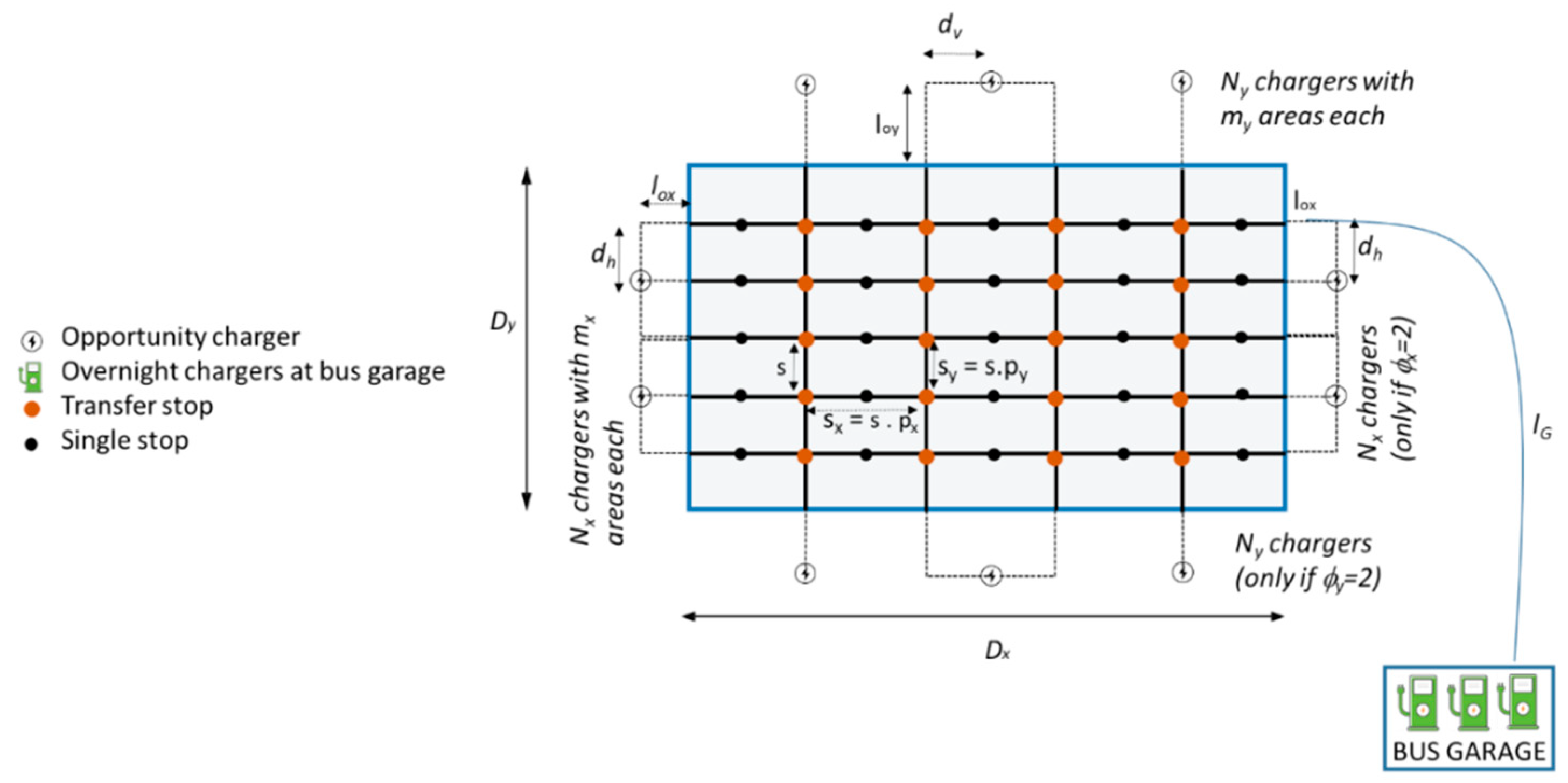
• Street network and bus corridor structure: It was assumed that buses follow a perfect grid configuration. Another assumption is that the city is covered by orthogonal bus corridors, traveling in the west–east and north–south axis and operated in two directions of service (see Figure 1). The headways of the corridors running along the horizontal and vertical directions (x and y axes) are denoted by H_x and H_y respectively. Moreover, the route spacing between the vertical or horizontal lines are respectively s_x = p_x·s and s_y = p_y·s, where s is the stop spacing and p_x, p_y two integer variables. Finally, there is a transfer stop at each intersection between vertical and horizontal routes. Hence, users can move in the network from any point to any other point with one transfer.
• User behavior and service characteristics: The network is designed to minimize the total cost at the peak hour, serving a total of Λ passengers with origins and destinations uniformly distributed in the service area D_x and D_y (in Estrada [25] it is stated that the agreement between the cost and performance estimations of continuous approximation models with OD simulation techniques is within 85%). However, the bus service will also be provided during Ω hours along the day, with an average hourly demand λ(pax/h). The door-to-door travel time of users integrates: the access and egress time spent at a v_w walking speed to/from the closest stop, waiting time at stops, riding time and the transfer time to overcome the distance δ between the loading platforms of orthogonal routes.
• Kinematic characteristics of buses: The maximal cruising speed on both horizontal and vertical lines is assumed to be identical and equal to v. Boarding and alighting time per passenger at stops is τ’. On the other hand, vehicles have a constant acceleration rate a and a maximal instantaneous speed of v_max. Therefore, the additional driving time to perform one stop with regard to one vehicle cruising at maximal speed (without stopping) is τ = v_max/a.
• Vehicle powertrains and energy provision: It was assumed that ICE-powered buses (diesel) or battery electric buses (BEB) would operate the service. In the case of diesel vehicles, the auxiliary facility to provide energy will be a set of fuel dispensers (fuel station) to be located in the bus garage.

On the other hand, if the service is provided by BEB vehicles, one of the crucial decision variables is the energy capacity of the battery pack (E, in kWh). In fact, it was assumed that vehicles must have, at any point of the service, enough energy to run a distance to the bus garage or maintenance location. Despite the fact that the city may present several bus garages scattered in the city periphery, it was assumed that the maximal distance to be run from terminal stop to the bus garage is l_G. This can be conceived as a distance margin that every bus may overcome in the necessary case. Assuming an average vehicle consumption factor of f_c (kWh/veh-km), the effective energy that can be used is (E − f_c·l_G). Therefore, it has to be check that the effective energy capacity (E − f_c·l_G) provides a sufficient autonomy range to operate the service all day long. If so, this vehicle will be charged at the bus garage during the night period. This operation is denoted as overnight charging.

The total number of chargers to be deployed at the bus garage for overnight charging is given by $n_{ch}=M/{\left[\frac{24-\mathsf{\Omega }}{E/S_D}\right]}^{-}$, where M is the fleet size (see Equation (12)) and [x]⁻ a mathematical operator that gives the lower integer of x. The term into brackets is, indeed, the number of buses that a single charging station is able to charge completely their batteries at full capacity (E) at an electric power S_D during the available night time. Otherwise, if BEB vehicles are equipped with small battery packs, it may be charged on-route. This operation is known as opportunity charging. From now on, it will be assumed that opportunity fast chargers are only located at terminal stops. The regular case considers that there are N_y charging stations evenly distributed along distance D_x in the North or the South periphery quadrant of the city.

Due to urban space scarcity, it was considered that all these stations are located a vertical distance l_oy far from the city boundary. Similarly, there are N_x stations located in the east or west periphery quadrant evenly distributed along D_y distance. All these N_x stations are situated l_ox distance away from the vertical boundary of the city. Therefore, vertical and horizontal corridors will have one terminal stop in each round trip where the battery charging operation is available. Nevertheless, it can be also considered that N_x and N_y additional charging facilities can also be deployed symmetrically in the opposite periphery quadrants, allowing buses to be charged at each terminal stop of each bus route direction. Doing this, vehicles may be equipped with smaller battery packs since bus charging operation may be more frequent than before. The E-W and N-S periphery quadrants with charging stations are controlled by decision variables ${\varphi }_x\mathrm{and}{\varphi }_y$. When these variables are equal to ${\varphi }_x=2;{\varphi }_y=2$, it means that charging stations are located in both periphery quadrants E-W and N-S.

Depending on the location of the chargers in W-E quadrants, the vehicles operating the last part of a horizontal corridor will run along a vertical detour distance $d_v$ to the charger. This distance is, in fact, a function of the number of chargers located at W-E quadrants,$d_v=$ $d_v\left(N_x\right)$. Similarly, vehicles operating vertical corridors will incur an extra horizontal distance $d_h=$ $d_h\left(N_y\right)$ based on the number of available chargers. Therefore, when ${\varphi }_x=2;{\varphi }_y=2$, the distance range between two charging operations in vertical and horizontal corridors are respectively denoted by d_c,S = d_c,N = D_y + 2 l_oy + $2d_h$, d_c,E = d_c,W = D_x + 2 l_ox +$2d_v$. They include respectively the longitudinal distance run within the city boundaries, the longitudinal distance travelled out of the city boundaries, and the detour distance in the transversal direction.

On the contrary, the situation described by ${\varphi }_x=1; {\varphi }_y=1$is equivalent to the regular case, where there is a charging station in just one terminal stop. In that case, the distance run is d_c,S = 2D_y + 2l_oy + $2d_h$ and d_c,E = 2D_x + 2l_ox + $2d_v$. Hence, the total number of charging stations to provide service in vertical and horizontal corridors is respectively ${\theta }_y{N}_y$ and ${\theta }_x{N}_x$. Note that when the charging time of a single bus at a terminal stop is higher than the target time headway H_x or H_y, vehicles cannot be dispatched at the required frequency unless multiple charging areas are deployed. Therefore, several buses must be charged simultaneously at the terminal stop. Hence, it was considered that each charging station y (y = 1, …, N_y) located in the N–S quadrants will be deployed with m_y charging areas. Each charging area has a parking slot for one bus and is equipped with an independent charging connector. Therefore, a total of m_y buses can be charged simultaneously at each charging station of the set N_y. Similarly, each charging station x (x = 1, …, N_x) located in E-W periphery quadrants will be equipped with m_x charging areas.

The number of charging areas in each charger station (m_x or m_y) is defined to be the minimal value that satisfies the required charging time and the dispatchment of vehicles at the target headways H_x or H_y. To do so, it was considered that the charging time of one vehicle at charging station y is $T_{c,y}$ (y = 1, …, N_y). In addition to that, it was considered that the expected number of routes served at each charging station is $\frac{D_x}{N_y{p}_{x}s}$. If the average headway between two consecutive bus departures from each charger y is ${\overline{h}}_y$, therefore the minimal number of charging areas that each terminal stop y in north and/or south peripheral quadrants must present is given by $m_y={\left[\frac{T_{c,y}}{{\overline{h}}_y}\right]}^{+}={\left[\frac{T_{c,y}}{H_y}\frac{D_x}{N_y{p}_{x}s}\right]}^{+}$. In the W-E periphery quadrants, the number of charging areas is similarly calculated by $m_x={\left[\frac{T_{c,x}}{H_x}\frac{D_y}{N_x{p}_{y}s}\right]}^{+}$. Therefore, the total number of opportunity charging areas is $n_{ch}=\left(m_x{\varphi }_x{N}_x+m_y{\varphi }_y{N}_y\right)$.

Another available charging alternative is the daily charging operation at the bus garage, where vehicles are charged at this facility during the service. As a difference from the opportunity and overnight charging, vehicles present very different levels of SOC during the service. The modeling approach in the following lines is developed for a horizontal route. Let ${\mu }_x=2D_x/\left(H_x·v_{cx}\right)$ be the number of vehicles needed to operate a single horizontal corridor to fulfill the target headway $H_x$. It was assumed that after $\Delta t_0$ units of time from the beginning of the service, a subset of $\mathsf{\Delta }{\mu }_x$ vehicles ($\mathsf{\Delta }{\mu }_x\le {\mu }_x$) will go to the bus garage to be charged. These vehicles will be replaced in the service by the same amount of extra vehicles that were previously parked at this facility, with batteries completely charged. These $\mathsf{\Delta }{\mu }_x$ vehicles will spend $l_G/v$ units of time traveling to the bus garage, $\Delta t_{0,x}·v_{c,x}·\frac{f_c}{S_d}$ units of time being charged (they have only provided service during $\Delta t_{0,x})$, and $l_G/v$ units of time for traveling again to the bus route to continue the service. Therefore, the time needed during this first cycle of charging is $\Delta t_{1,x}=\frac{2l_G}{v}+\Delta t_{0,x}·v_{c,x}·f_c/S_d$. At time $\Delta t_{0,x}+\Delta t_{1,x}$, we can start the second cycle of charging, replacing those $\mathsf{\Delta }{\mu }_x$ vehicles pending to be recharged, by the ones coming from the bus garage. Note that the charging operation of these second group of vehicles needs $\Delta t_{2,x}=\frac{2l_G}{v}+\left(\Delta t_{0,x}+\Delta t_{1,x}\right)·v_{c,x}·f_c/S_d$ units of time to be reintroduced again into the service. Generally, the $\mathsf{\Delta }{\mu }_x$ vehicles replaced at the n-th cycle of charging will consume $\Delta t_{n,x}=\frac{2l_G}{v}+\left({\displaystyle \sum }_{i=0}^{n-1}\Delta t_{i,x}\right)·v_{c,x}·\frac{f_c}{S_d}$ units of time for being available again. Therefore, this charging scheme may charge vehicles during the whole service at the expense of deploying $\mathsf{\Delta }{\mu }_x$ additional vehicles in the operation, and performing the unproductive trips between routes and bus garage.

The variables that control the charging operations are the number of charging cycles performed (${\pi }_x$), the number of extra vehicles $\left(\mathsf{\Delta }{\mu }_x\right)$ and the elapsed time when the first charging operation is performed ($\Delta t_{0,x}$). In order to ensure a feasible charging scheme, it has to fulfill on one hand that all charging cycles are performed within the service period (${\displaystyle \sum }_{i=0}^{{\pi }_x}\Delta t_{i,x}\le \mathsf{\Omega }$) and, secondly, the added vehicles and the number of charging cycles are enough to charge all vehicles operating the route (${\pi }_x·\mathsf{\Delta }{\mu }_x\ge {\mu }_x$). Similar equations must be fulfilled in the vertical corridors (y coordinate). Consequently, the bus network design problem is aimed at minimizing the total costs of the system (Z), defined by Equation (1).

$$\underset{\begin{array}{c}s, H_x,H_y,px,py,\\ Nx, Ny,{\varphi }_x, {\varphi }_y\end{array}}{\min }\left\{Z=\left[c_{L}L+c_N{n}_{ch}\right]+\left[c_{V}V+c_{M}M+c_{B}E\times M\right]+\left[\mathsf{\lambda }{\beta }_{T}T\right]+\left[Z_E\right]\right\}$$

(1)

$$\mathrm{subject}\mathrm{to}$$

$$O_x\le C$$

(2a)

$$O_y\le C$$

(2b)

$$\max \left(v_{c,x},v_{c,y}\right)\times \mathsf{\Omega }+l_G\le \frac{E}{f_C}$$

(3a)

$$\max \left({{\displaystyle \sum }}_{i=0}^{{\pi }_x-1}\Delta t_{i,x}\times v_{c,x},{{\displaystyle \sum }}_{i=1}^{{\pi }_x}\Delta t_{i,x}\times v_{c,x},{{\displaystyle \sum }}_{i=0}^{{\pi }_y-1}\Delta t_{i,y}\times v_{c,y},{{\displaystyle \sum }}_{i=1}^{{\pi }_y}\Delta t_{i,y}\times v_{c,y}\right)\le \frac{E}{f_C}$$

(3b)

$$d_{c,W}+l_G,d_{c,E}+l_G,d_{c,N}+l_G,d_{c,S}+l_G<\frac{E}{f_C}$$

(3c)

$$s\ge s_{min};H_x,H_y\ge H_{min}$$

(4)

$$s,H_x,H_y\in {ℝ}^{+}$$

(5)

$$N_x,N_y\in \mathbb{N}$$

(6)

$$p_x,p_y,{\varphi }_x,{\varphi }_y=\left\{1,2\right\}$$

(7)

The first term in brackets in Equation (1) captures the infrastructure cost that the transit agency will incur, where L is the total length of bus corridors (two ways of service) and $n_{ch}$ the number of electric charging areas (BEB vehicles) or the number of refueling stations (ICE vehicles). The corresponding parameters $c_L$and $c_N$ determine the depreciation cost per unit of bus lane distance, and per unit of charging area and hour respectively. In the case of diesel vehicles, $c_N$ is calculated as the depreciation cost of one fuel station per hour, divided by the number of refueling operations that a single station can perform along the night period.

The second term in brackets estimates the agency’s operating cost. The total distance run by the fleet in one hour (V) and the fleet needed (M) are multiplied by the corresponding unit distance cost (c_V) and unit temporal cost (c_M). The former considers all operating costs depending on the distance run (mainly energy), while c_M embraces vehicle depreciation, driver salary, insurances and other fixed expenses. Typically, the depreciation cost of electric buses does not encompass the depreciation cost of batteries ($c_B$), since the battery lifetime is significantly lower than the vehicles. Indeed, the battery capacity (E) has to be determined, according to the route length and energy consumption factors.

Moreover, the user cost contribution is calculated in the third bracketed term by the product of the average hourly demand rate ($\lambda$ in pax/h), the value of time (${\beta }_T$ in USD/pax-h) and the total door-to-door travel time (T, in hours). This travel time component encompasses access (A), waiting (W), transfer (Tr) and in-vehicle travel time (IVTT). Finally, it was also included in the objective function the monetary cost of emissions per hour of service (Z_E). Therefore, the total cost function Z (USD/h), in terms of monetary units per hour of service.

Equations (2a) and (2b) constraint that the occupancy of vehicles running along x and y directions ($O_x$ and $O_y$ respectively) should be lower than the maximal passenger capacity of buses (C in pax/bus). The set of Equation (3) is aimed at verifying that vehicles present a sufficient range under three charging schemes. If we opted for an overnight charging scheme at the bus garage, Equation (3a) states that the total distance run along the whole day by BEB vehicles, plus a safety margin distance $l_G$, should be lower than the maximal allowable distance ($E/f_C$). In the former equation, $v_{c,x} \mathrm{and} v_{c,y}$ represent the number of kilometers run per hour in the x and y direction by a single bus (net commercial speed calculated through Equations (11a) and (11b). Equation (3b) ensures a sufficient range for the group of vehicles charged at the first (i = 1) and last cycle (i = ${\pi }_x$ or ${\pi }_y$) of charging at the bus garage during the service. Similarly, Equation (3c) should be only satisfied by BEB technology with the opportunity charging scheme. Equation (4) constraints the minimal threshold of stop spacing ($s_{min}$) and headways ($H_{min}$). It was assumed that below these two thresholds, buses would stop too frequently along the route or they would not be able to maintain an acceptable headway adherence. Finally, constraints (5)–(7) specify the feasible domains and the nature of the decision variables. Indeed, it was restricted that routes will be spaced, at most, twice the stop distance.

In the following subsections, it will calculate each component of the objective function dependent on the decision variables of the problem: s, H_x, H_y, p_x, p_y, N_x, N_y, $\varphi$_x and $\varphi$_y.

Bus agency metrics

The different cost components incurred by transit agencies are estimated, considering similar approaches presented in Daganzo and Estrada [17,25]. Equation (8) captures the total bidirectional length of the network (L), while Equation (9) estimates the distance run in one hour by the whole fleet (V). It was assumed that in the case of BEB vehicles with opportunity charging scheme, each vehicle operating a horizontal corridor runs an extra distance l_ox + $d_v$ from the terminal stop to the closest charging station. This extra distance is equal to $l_{oy}+d_h$ for vehicles running along vertical corridors. In diesel and BEB powertrains, $l_{ox}=d_v=l_{oy}=d_h=0$. In the case of day charging at the bus garage, the terms ${\displaystyle \sum }_{i=0}^{{\pi }_x}\Delta t_{i,x}$ and ${\displaystyle \sum }_{i=0}^{{\pi }_y}\Delta t_{i,y}$ represent the time needed to charge all vehicles starting the service (one charging cycle) in the horizontal and vertical corridors. In other charging schemes and diesel powertrains, these terms must be ${\displaystyle \sum }_{i=0}^{{\pi }_x}\Delta t_{i,x}={\displaystyle \sum }_{i=0}^{{\pi }_x}\Delta t_{i,x}=\infty .$ Moreover, it was calculated the expected number of transfers $p\left(1\right)$per user through Equation (10). This variable is needed to compute the net commercial speed $v_c$ in x and y coordinates, addressed in Equation (11). The net commercial speed is the average speed that buses will experience to perform a complete round trip of length $2D_x$ (horizontal) or $2D_y$ (vertical). In the case of BEB with opportunity charging scheme, the total length is computed by 2$\left(D_x+l_{ox}+d_v\right)$ (horizontal) or $2\left(D_y+l_{oy}+d_h\right)$ (vertical). The net commercial speed takes into account the lay-over time at terminal stops (${\theta }_E,{\theta }_W,{\theta }_S,{\theta }_N$) and the charging time $T_{c,z}$ spent at the corresponding terminal station z (z = W, E, S or N) only by BEB vehicles. Finally, the fleet size needed to run the service is addressed by means of Equation (12).

$$L=D_y{D}_x\left(\frac{1}{p_{y}s}+\frac{1}{p_{xy}s}\right)$$

(8)

$$\begin{gathered} V=2D_y{D}_x\left(\frac{1}{H_x{p}_{y}s}+\frac{1}{H_y{p}_{x}s}\right)+\frac{2D_y}{H_x{p}_{y}s}\left(l_{ox}+d_v+\frac{2l_G{D}_x}{v_{c,x}{{\displaystyle \sum }}_{i=0}^{{\pi }_x}\Delta t_{i,x}}\right) \\ +\frac{2D_x}{H_y{p}_{x}s }\left(l_{oy}+d_h+\frac{2l_G{D}_y}{v_{c,y}{{\displaystyle \sum }}_{i=0}^{{\pi }_y}\Delta t_{i,y}}\right) \end{gathered}$$

(9)

$$P\left(1\right)=1-\frac{p_{x}s{D}_y+p_{y}s{D}_x-p_x{p}_y{s}^2}{D_x{D}_y}$$

(10)

$$\frac{1}{v_{c,x}}=\frac{1}{v}+\frac{1}{s}\tau +\frac{\frac{\mathsf{\Lambda }}{2}{H}_x\left[1+p\left(1\right)\right]{\tau }^{\prime }}{2D_y\left(D_x+l_{ox}+d_v\right)/\left(p_{y}s\right)}+\frac{{\theta }_E+{\theta }_W+\max \left\{0,T_{c,E}-{\theta }_E\right\}+\max \left\{0,T_{c,W}-{\theta }_W\right\}}{D_x+l_{ox}+d_v}$$

(11a)

$$\frac{1}{v_{c,y}}=\frac{1}{v}+\frac{1}{s}\tau +\frac{\frac{\mathsf{\Lambda }}{2}{H}_y\left[1+p\left(1\right)\right]{\tau }^{\prime }}{2D_x\left(D_y+l_{oy}+d_h\right)/\left(p_{x}s\right)}+\frac{{\theta }_S+{\theta }_N+\max \left\{0,T_{c,S}-{\theta }_S\right\}+\max \left\{0,T_{c,N}-{\theta }_N\right\}}{D_y+l_{oy}+d_h}$$

(11b)

$$M=\frac{2D_y}{{\left(v_c\right)}_x{H}_x{p}_{y}s}\left(D_x+l_{ox}+d_v\right)+\frac{2D_x}{{\left(v_c\right)}_y{H}_y{p}_{x}s}\left(D_y+l_{oy}+d_h\right)+\mathsf{\Delta }{\mu }_x\frac{D_y}{p_{y}s}+\mathsf{\Delta }{\mu }_y\frac{D_x}{p_{x}s}$$

(12)

In the case of BEB with the opportunity charging scheme, the charging time $T_{c,z}$ spent at terminal station z is calculated in Equation (13), where z represents the charging stations located on the north, south, east and west part of the city. The first term is the minimal charging time whose estimation is based on the energy consumed in the distance run from the last charging operation d_c,z, the energy consumption factor f_c and the charging speed S_D. The second term captures the positioning and clearance time spent at the charging area per bus in the terminal stop, $t_{pos}$. This time is neglected in alternative solutions that do not visit the on-street opportunity charging facility ($T_{c,z}$ = 0).

$$T_{c,z}=\frac{d_{c,z}{f}_c}{S_D}+t_{pos}$$

(13)

User metrics

The expected door-to-door travel of a single user T is calculated as the summation of access (A), waiting (W), transfer (Tr) and in-vehicle travel time (IVTT) through Equations (14)–(17) respectively. Equation (15) the estimation of the waiting time specifies the different headway provision along directions x and y. Moreover, the IVTT term must take into account the gross commercial speed of buses $v_c’$, i.e., the average commercial speed experienced by users, neglecting the idle time spent at the terminal stops. Finally, Equation (18) defines the expected passenger occupancy in the vehicles operating routes in the x and y directions.

$$A=s\left(\frac{2+p_x+p_y}{2v_w}\right)$$

(14)

$$W=\left(1-p\left(1\right)\right)\times \frac{H_x+H_y}{4}+p\left(1\right)\frac{H_x+H_y}{2}$$

(15)

$$T_{TR}=\frac{\delta ·p\left(1\right)}{v_w}$$

(16)

$$IVTT=\frac{D_x+D_y}{3}\left(\frac{1}{v}+\frac{1}{s}\tau \right)+\frac{\mathsf{\Lambda }s\left[1+p\left(1\right)\right]{\tau }^{\prime }\left(D_x{H}_x{p}_y+D_y{H}_y{p}_x\right)}{12D_y{D}_x}$$

(17)

$$O_x=\frac{\mathsf{\Lambda }}{16}\left(1+p\left(1\right)\right)\frac{s_y}{D_y}{H}_x{O}_y=\frac{\mathsf{\Lambda }}{16}\left(1+p\left(1\right)\right)\frac{s_x}{D_x}{H}_y$$

(18)

Emissions

The estimation of the local emissions and greenhouse gases (GHGs) generated within all the processes needed to run the bus service is addressed in this section. These emissions have been calculated by means of a lifecycle analysis of the vehicle manufacturing, infrastructure construction and the well to wheel analysis of the energy required to operate the vehicles, given a bus powertrain and bus size. These contributions are estimated by means of the corresponding emission factor of a specific pollutant generated by one process (vehicle operation, manufacturing and infrastructure construction). These factors will be later multiplied by the corresponding size fleet (M), infrastructures (L and n_ch) and distance run (V) in one hour of service.

The local pollutants considered are PM₁₀, SO_x, CO, NO_x, NH₃ and VOC, while CO₂, CH₄ and N₂O are transformed into CO₂ eq to account for GHG, taking the corresponding warming potentials. Both local pollutants and CO₂ eq constitute the set P of different emission typologies considered in this paper. Finally, the mass of each pollutant generated per hour of service has been monetized to be integrated in the objective function. To do so, a proxy parameter ${\epsilon }_p$ has been defined to monetize the effect of producing one unit of pollutant p $\in$ P. The values of these proxy parameters (in USD/g of pollutant p) were determined according to van Essen et al. [40]. The processes considered that have an associated economic impact in terms of emissions and pollutants in the bus system are the following:

Monetization of the emissions caused by the circulation of vehicles: Z_e,F: Each ICE vehicle produces $E_{F,p}$ (g/veh-km) grams of local pollutant p (p $\in$ P) per kilometer run. In fact, these emission factors capture the pollutants generated in the tank-to-wheel phase. These emission factors, in reality, depend on the type of vehicle, speed regime, driving style and fuel consumption factors [33]. The emission monetization associated to the circulation of vehicles in one hour can be estimated by Equation (19), taking into account the total distance run by the whole fleet (V) in the peak hour. It is considered that BEBs do not present any pollutant contribution.

$$Z_{e,F}=V\times {\displaystyle \sum }_{p\in P}{E}_{F,p}{\epsilon }_p$$

(19)

Monetization of the emissions caused by the energy generation in production plans: Z_e,E: The generation of electricity from primary energy sources for bus battery charging also lead to emissions when the service is operated by BEBs. These emissions, in both BEB and ICE vehicles, are estimated by means of the well-to-tank analysis. The emission factor E_E,p of pollutant p (g of pollutant p/kWh) is estimated as the mass of this pollutant caused in the generation and transportation of one unit of energy to move vehicles. These emission factors depend on the energy mix of the country. Equation (20) captures the estimation of the Z_e,E variable, where $f_c$ (kWh/veh-km) represents the energy consumption factor of the bus fleet.

$$Z_{e,E}=V\times f_c{\displaystyle \sum }_{p\in P}{E}_{E,p}{\epsilon }_p$$

(20)

Monetization of the emissions caused by vehicle manufacturing and maintenance: Z_e,M: The manufacturing of public transport vehicles consumes and transforms a wide number of raw and semiprocessed materials. The emission factor of pollutant p, E_M,p (g of pollutant p/veh-h) is defined as the ratio among the total amount of emissions of this pollutant p in the vehicle production and maintenance and the number of working hours along the vehicle lifetime. The emission monetization of this effect is obtained by Equation (21), multiplying emission factors by the proxy parameters $({\epsilon }_p)$ and the fleet size (M).

$$Z_{e,M}=M\times {\displaystyle \sum }_{p\in P}{E}_{M,p}{\epsilon }_p$$

(21)

Monetization of the emissions caused by the row infrastructure construction: Z_e,I: The manufacturing of the infrastructure needed to build that transit lane also contribute to the GHG and local emissions. In that case, the emission factor for pollutant p is considered per unit of infrastructure length and unit of time used, E_I,p (g/km-h). It was also accounted for the contribution of public work machinery used in the whole construction phase of the bus network. The total amount of emissions produced in one kilometer is split along the target lifetime of the infrastructure. Then, the monetization can be obtained by Equation (22).

$$Z_{e,I}=L\times {\displaystyle \sum }_{p\in P}{E}_{I,p}{\epsilon }_p$$

(22)

Monetization of the emissions caused by the stop/station construction: Z_e,S: This term encompasses the economic effects of the emissions generated in the construction of stops, stations and charging stations. Traditionally, the material and energy consumption in the construction of the bus stop was significantly lower than the bus lane infrastructure. It was assumed that E_S,p (g/st-h) and E_C,p (g/st-h) are the emission factors of pollutant p per hour of stop and electric charging area respectively. The emissions caused by the construction of refueling stations for diesel vehicles at bus garage are considered in the $E_{E,p}$ term, and therefore they were not addressed here. Consequently, the term Z_e,S can be calculated by Equation (23).

$$Z_{e,S}=\frac{D_x{D}_y}{p_x{p}_y{s}^2}\times {\displaystyle \sum }_{p\in P}{E}_{S,p}{\epsilon }_p+n_{ch}\times {\displaystyle \sum }_{p\in P}{E}_{C,p}{\epsilon }_p$$

(23)

Optimization procedure

The analytical model presented before allows identifying the optimal design of the public transport network from 5 decision variables for ICE powertrains, or for BEB powertrain when overnight charging is chosen: headways in horizontal and vertical routes, stop spacing and route spacing between vertical and horizontal lines defined by the auxiliary variables p_x and p_y. Nevertheless, in the case of the deployment of electric bus technologies with opportunity charging, four additional decision variables are considered to account for the number of electric charging stations and charging areas in the N–S periphery (θ_y, N_y) or in the E-W periphery (θ_x, N_x). The optimization process followed in this paper was based on a grid enumeration of the objective function, in relation to the decision variables. For each of the variables with a continuous domain, it was identified an enumeration interval pace (Δs and ΔH) to discretize the enumeration domain. The discretized domain of these variables is therefore enumerated by $s=s_{min}+k_s{\Delta }_s$ and $H_x=H_{min}+k_H{\Delta }_H$, $H_y=H_{min}+k_V{\Delta }_H;k_s,k_H,k_V=0,\mathrm{..},k_{max.}$ Input parameters $s_{min}$, $H_{min}$ define the minimal reasonable value of stop spacing and time headway respectively, while $k_{max}$ is defined based on the maximal value of the former decision variables. In the case of the discrete variables, the enumeration domain of p_x, p_y and $\varphi$_x, $\varphi$_y was {1, 2}, while the corresponding to the number of chargers was N_x = {1, 2, …, $\frac{D_y}{s·p_x}$} and N_y = {1, 2, …, $\frac{D_x}{s·p_y}$}. Therefore, the total cost of the collective transport system Z (s’, H’, p_x’, p_y’, N_x’, N_y’, $\varphi$_x’, $\varphi$_y’) is evaluated by Equation (1) for each potential combination of decision variables defined in the grid search. Hence, the feasible solution of the optimization problem stated in Equation (1) is the combination of decision variable values that produce the minimal cost of the objective function (Z), satisfying the constraints of Equations (2)–(7).

2.2. Materials

The applicability of the model presented has been tested under various scenarios of bus powertrains in Guadalajara, México (Figure 2). The city of Guadalajara, located in the Jalisco state, is the second most populated city in Mexico, with near to 5 million inhabitants within its metropolitan area spread in an area of 151.6 km² [41].

Public transport services the Guadalajara Metropolitan Area by means of a door-to-door bus network, operated by 12 m-long diesel buses. The bus service area has been modeled by a rectangle of sides D_x × D_y = 18·15 km². The peak hour demand of bus passengers in a working day was estimated to be Λ = 333,613 pax/h, while the average hourly demand considering the variability along the whole day was λ = 236,605 pax/h. Both figures have been calculated from the data provided in Parada [42]. Moreover, it was assumed that the value of time of passengers using the bus service in Guadalajara is μ = 3.14 USD/pax-h, considering that the average monthly salary in 2018 was 514 USD [43]. It was assumed that these users show an average walking speed of v_w = 4.5 km/h and the average transfer distance between loading areas at stops is δ = 0.3 km [25]. The service is provided along $\mathsf{\Omega }=$ 16 h per day.

The infrastructure cost to build the bus lane along the transit corridors was supposed to be c_L = 84.36 USD/km-h [23]. Eight scenarios regarding different vehicle capacities, powertrains and charging operation are considered in the analysis:

• C-12. Standard bus with diesel engine (12 m long, conventional environmental label);
• C-18. Articulated bus with diesel engine (18 m long, conventional environmental label);
• EuroVI-12. Standard bus with diesel engine (12 m long, Euro VI environmental label);
• EuroVI-18. Articulated bus with diesel engine (18 m long, Euro VI environmental label);
• BEB-12 Ov. Standard battery-electric bus with overnight charging (12 m long);
• BEB-12 Opp. Standard battery-electric bus with opportunity charging (12 m long);
• BEB-12 Day. Standard battery-electric bus with charging at the bus garage during service (12 m long);
• BEB-18. Articulated battery-electric bus with opportunity charging (18 m long).

The scenario C-12 represents the current standard size (12 m long) and diesel vehicle powertrain use in Guadalajara, without significant treatments of emissions (conventional diesel). A similar scenario entitled C-18 was created for articulated diesel buses (18 m long) with the same conventional environmental label but higher passenger capacity. Scenarios EuroVI-12 and EuroVI-18 will consider a situation with the most recent diesel-hybrid technology. They differ in terms of the vehicle typology, and consequently, in the maximal passenger occupancy that they can accommodate. Finally, the last four scenarios suppose that charging facilities and BEB vehicles would be deployed. For standard buses of 12 m of length, it was considered that overnight charging at the bus garage, day charging at the bus garage during service and opportunity charging at terminal stops are feasible. For articulated buses of 18 m, only the opportunity charging operation was considered in the analysis.

The vehicle capacities of all standard and articulated buses are respectively C = 70 pax and C = 120 pax. It was assumed that buses of all the scenarios present the same cruising speed v = 30 km/h, unit boarding and alighting time per passenger $\tau ’$ = 3 s [18], and the additional running time to perform one stop due to acceleration and deceleration phase is $\tau =\frac{v}{a}$ = 35 s. On the other hand, the maximal acceleration/deceleration rate is a = 0.85 m/s² [44]. The parameters that depend on the vehicle typology are summarized in

Table 1. Input parameters.

Cost Parameters		Standard Bus, 12 m Long				Articulated Bus, 18 m Long
		Diesel Diesel		Electric		Diesel Diesel		Electric
		Conventional	EURO VI	Over-n./Day	Oppor-tunity	Conventional	EURO VI	Oppor-tunity
Energy consumption factor (kWh/veh-km)		6.207	4.746	1.400		7.689	6.304	1.900
Unit energy cost (USD/veh-km)	(a)	0.685	0.524	0.112		0.849	0.696	0.152
Spare parts, maintenance staff cost (USD/veh-km)	(b)	0.254	0.254	0.169		0.293	0.293	0.163
Unit distance cost,${\mathit{c}}_{\mathit{V}}$(USD/veh-km)	(a + b)	0.940	0.778	0.281		1.142	0.989	0.315
Unit driver cost, (USD/veh-h)	(c)	9.450	9.450	9.450		9.450	9.450	9.450
Vehicle acquisition cost (USD/veh)		198,000	277,500	555,000		275,000	385,000	876,900
Amortized Vehicle cost (USD/veh-h)	(d)	2.500	3.504	7.008		3.472	4.861	11.072
Refuel workload at bus garage (USD/veh-h)	(e)	0.183	0.083	0.000		0.183	0.183	0.000
Insurances, control, engineering staff (USD/veh-h)	(f)	2.626	2.626	2.964		2.626	2.626	2.626
Unit temporal cost,${\mathit{c}}_{\mathit{M}}$(USD/veh-h)	(c + d + e + f)	14.759	15.663	19.421		15.731	17.120	23.148
Charger facility/Fuel station invest.(kUSD)		5550	5550	95.87	777	5550	5550	777
Vehicle capacity of the charger/station (veh)	(g)	350	350	1	1	350	350	1
Facility cost (USD/charger-h)	(h)	35.04	35.04	0.605	5.396	35.04	35.04	5.396
Charger/Refuel station maintenance cost (USD/facility-h)	(i)	1.354	1.354	0.625	0.625	1.354	1.354	0.625
Unit energy facility cost or refueling station, cN (USD/charger-h)	(h + i)/(g)	0.104	0.104	1.230	6.021	0.104	0.104	6.021
Unit battery cost, cb (USD/kWh-h)		--	--	0.0190		--	--	0.019
Aggregated Tank to Wheel emission monetization, ${\displaystyle \sum }_{p\in P}{E}_{F,x}{\epsilon }_p$(USD/veh-km)		0.9015	0.1580	0		1.1434	0.2027	0
Aggregated Well to Tank emission monetization, ${\displaystyle \sum }_{p\in P}{E}_{E,p}{\epsilon }_p$(USD/kWh)		0.0106	0.0106	0.0974		0.0106	0.0106	0.0974
Aggregated Vehicle manuf. emission monetization, ${\displaystyle \sum }_{p\in P}{E}_{M,p}{\epsilon }_p$(USD/veh-h)		0.1598	0.1598	0.2008		0.2157	0.2157	0.2711
Aggregated Infrastructure emission monetization, ${\displaystyle \sum }_{p\in P}{E}_{I,p}{\epsilon }_p$(USD/km-h)		0.1089	0.1089	0.1089		0.1089	0.1089	0.1089
Aggregated Charger emission monetization, ${\displaystyle \sum }_{p\in P}{E}_{C,p}{\epsilon }_p$(USD/char-h)		--	--	0.0171				0.0171

. The driver cost component (Table 1, row c) was reported to be 9.45 USD/veh-h in Guadalajara, considering the current salaries [45]. The unit distance cost of the ICE vehicles in the first four scenarios was calculated considering the cost of the diesel consumption [32], and an additional cost term that accounts for vehicle maintenance staff and spare parts.

The latter cost component (row b), refuel workload (row e) and engineering staff (row f in Table 1) were calculated considering the real cost reported in Barcelona by Transportes Metropolitanos de Barcelona (TMB) [46] and multiplied by the ratio η_GB = 0.2505. This ratio, calculated as the driver cost in Guadalajara divided by the corresponding value in Barcelona (37.72 Euro/veh-h), accounts for the different labor regulations, salaries and monetary parity between these cities. The vehicle purchasing costs, charger and refueling station investments are supposed to be equivalent to the figures reported in TMB [46]. The corresponding cost per hour of vehicle or hour of facility were calculated through a linear amortization along 79,200 h (15 years·330 day/year·16 h/day). The cost of each refueling station is divided by the number of buses whose fuel tank can be refilled in the same day (350 buses), and expressed in terms of USD/veh-h. It is worth to mention that the investment in the charging stations for standard buses at the bus garage is significantly lower than the corresponding to buses charged on the street (opportunity charging).

The battery cost presents a significant variability depending on the different available chemistries, lifespans and acquisition conditions. Organization for Economic Co-operation and Development and International Energy Agency (OCDE-IEA) [45] suggests that the battery cost should range between 120 and 400 USD/kWh in all BEB analysis. Indeed, they suggest a normal value of 260 USD/kWh. Nevertheless, in our study, the resulting battery cost was calculated as a straight-line depreciation of the maximal purchasing cost threshold 400 USD/kWh, along a lifetime of 4 years.

The unit emission costs (${\epsilon }_p$) and emission factors $(E_{F,p},E_{E,p},E_{M,p},E_{I,p},E_{C,p}$) for each pollutant p $\in P$, effect and vehicle scenario in the case applicability in Guadalajara are presented in detail in the

Table A1. Monetary values and emission factors corresponding to each pollutant.

		CO2	PM10	NOX	CO	SOX	VOC	NH3
C-12	Monetization x (USD/g polluntant x)	1.12 × 10−4	1.38 ×10−1	2.39 × 10−2	1.34 × 10−3	1.22 × 10−2	1.34 × 10−3	1.96 × 10−2
	Tank to Wheel, EF,x (g/km)	1.67 × 103	1.21	2.23 × 101	8.42	3.14 × 10−3	2.88	2.90 × 10−3
	Well to Tank, EE,x (g/kWh)	5.51 × 101	1.13 × 10−2	9.76 × 10−2	4.49 × 10−2	3.27 × 10−2	2.63 × 10−2
	Vehicle manufacturing, EM,x (g/veh-h)	1.43 × 103
	Infrastructure, EI,x (g/km-h)	6.19 × 102				3.24
Euro-VI 12	Tank to Wheel, EF,x (g/km)	1.28 × 103	8.11 × 10−3	5.28 × 10−1	3.64 × 10−1	2.40 × 10−3	5.70 × 10−2	9.00 × 10−3
	Well to Tank (g/kWh)	5.51 × 101	1.13 × 10−2	9.76 × 10−2	4.49 × 10−2	3.27 × 10−2	2.63 × 10−2
	Vehicle manufacturing, EM,x (g/veh-h)	1.43 × 103
	Infrastructure, EI,x (g/km-h)	6.19 × 102				3.24
C-18	Tank to Wheel, EF,x (g/km)	2.07 × 103	1.52	2.87 × 101	1.11 × 101	3.89 × 10−3	2.99	2.90 × 10−3
	Well to Tank, EE,x (g/kWh)	5.51 × 101	1.13 × 10−2	9.76 × 10−2	4.49 × 10−2	3.27 × 10−2	2.63 × 10−2
	Vehicle manufacturing, EM,x (g/veh-h)	1.93 × 103
	Infrastructure, EI,x (g/km-h)	6.19 × 102				3.24
Euro VI 18	Tank to Wheel, EF,x (g/km)	1.70 × 103	9.15 × 10−3	4.38 × 10−1	4.14 × 10−1	3.19 × 10−3	6.5 × 10−2	9.0 × 10−3
	Well to Tank, EE,x (g/kWh)	5.51 × 101	1.13 × 10−2	9.76 × 10−2	4.49 × 10−2	3.27 × 10−2	2.63 × 10−2
	Vehicle manufacturing, EM,x (g/veh-h)	1.93 × 103
	Infrastructure, EI,x (g/km-h)	6.19 × 102				3.24
BEB 12 Ov and Opp.	Tank to Wheel, EF,x (g/km)
	Well to Tank, EE,x (g/kWh)	5.14 × 102	8.58 × 10−2	8.02 × 10−1	2.55 × 10−1	6.90 × 10−1	6.29 × 10−2
	Vehicle manufacturing, EM,x (g/veh-h)	1.79 × 103
	Infrastructure, EI,x (g/km-h)	6.19 × 102				3.24
	Chargers (g/charger), EC,x (g/charger-h)	1.12 × 102	1.04 × 10−6	1.24 × 10−1	1 × 10−1	1.16 × 10−1	8.16 × 10−6	2.78 × 10−6
BEB-18 Opp	Tank to Wheel, EF,x (g/km)
	Well to Tank, EE,x (g/kWh)	5.14 × 102	8.58 × 10−2	8.02 × 10−1	2.55 × 10−1	6.90 × 10−1	6.29 × 10−2
	Vehicle manufacturing, EM,x (g/veh-h)	2.42 × 103
	Infrastructure, EI,x (g/km-h)	6.19 × 102				3.24
	Chargers (g/charger), EC,x (g/charger-h)	1.12 × 102	1.04 × 10−6	1.24 × 10−1	1 × 10−1	1.16 × 10−1	8.16 × 10−6	2.78 × 10−6

in the Appendix B. The unit emission costs parameters were considered the average values of contingency cost proposed by van Essen et al. [40] for the 28 European Union countries. In the case of CO₂ eq, the monetization factor was considered ${\epsilon }_{CO2}=111USD/TonC{O}_2$ based on the impact and wears on the territory. Reasonably, it is one order of magnitude greater than the figure proposed in SENDECO, since the latter is based on the market equilibrium price of CO₂ emission rights among countries.

The terms $E_{F,p}$ accounting for the tank-to-wheel emissions are calculated considering EEA using the Tier 3 estimation for the urban buses standard 15–18 t and urban buses articulated >18 t (diesel conventional and diesel EURO VI diesel powertrains), when the road slope is 0 and it is fully loaded. The non-exhaust emissions like fuel evaporation or emissions generated in the brake operations are not considered. Therefore, the corresponding emissions factors of this category for electric buses are considered to be 0. The emissions $E_{E,p}$ produced in the energy generation and transportation for diesel and battery electric bus powertrains within the well-to-tank phase were calculated using the GREET© fuel cycle model v2019 [30]. It considered the electricity mix for Mexico in 2014 published in IEA [47] based on the following primary energy sources: coal 11.3%, oil 11%, gas 57.1%, nuclear 3.3%, hydro 13%, bioenergy 0.3% and others clean sources (4%).

The emissions E_M,p caused by the vehicle manufacturing process are approximated to the results presented in Nordelöf et al. [35] for standard diesel and electric buses, based on the data of Volvo’s 7900 model series. The corresponding values for articulated buses were supposed to be 1.35 times higher than the values for standard buses. The emissions were split by a total vehicle lifetime of 15 years (diesel and electric), assuming 330 days of work along the year and 16 working hours per day.

On the other hand, the emissions E_I,p caused by the infrastructure construction were calculated based on Wayman et al. [48] to build 1 square meter of pavement surface. Assuming a lifespan of 60 years (including maintenance works, 360 days·16 h of service/day) and a bus lane width of 3.5 m, the CO₂ and SO₂ emissions were calculated per hour and kilometer of bus lane. Emissions factors of other pollutants were not available. Finally, the emissions factors associated to each stop construction were negligible in our analysis due to the minor requirements of bus shelters in Guadalajara.

Nevertheless, the emission factors for charging facilities were calculated based on Nansai et al. [49] regarding the installation and manufacturing phase of one charger (14.55 Ton CO₂, 16 kg NO_x, 15 kg SO_x and 13 kg CO). Additionally, it was also considered the emissions of the charger transportation along 40 km from the assembling plant to the final location with a heavy diesel duty truck 14–20 t (EURO VI). For each effect, the summation for all pollutants p of the corresponding emission factor, times the unit emission cost is summarized in Table A1. In the case of pollutant x = CO₂ eq, the emission factors considering the vehicle manufacturing, operation and the well to tank phase in Scenarios C-12, Euro VI 12 and BEB 12 Ov. are 3153, 2763 and 2306 g CO₂/veh-km (see Appendix B). In the case of the electric vehicle (Scenario 5), the well to tank emission factor is 514 g/kWh, similar to the 582 g/kWh for México [50].

3. Results

This section shows the final results derived from the model. Figure 3 shows the total cost of the bus system obtained by the optimization model in different powertrain scenarios, and in the current Guadalajara bus network configuration, operated by conventional standard (12 m) diesel buses.

Figure 3 indicates the total cost of each powertrain scenario expressed in USD/hour of service. Total cost integrates: user cost, agency cost, emission cost ad in the electric cases battery cost. On the other hand, Figure 4 summarized the design variables (p_x, p_y, s, H_x and H_y) and more performance metrics for each scenario.

Figure 4 is divided in two sections. The section above shows the decision variables, which are p_x, p_y, s, H_y and H_x. Each group of lectures corresponds to each of the powertrain scenario proposed. On the other hand the below section indicates the performance metrics of each scenario taking some of the main metrics such as the size of the fleet (M), waiting time (W), the total distance run by the fleet in one hour (V), longitude of the network (L) and in-vehicle travel time (IVTT).

3.1. Sensitivity Analysis

In this section, it was analyzed how the total cost of the system and the service performance metrics evolve in the different powertrain scenarios according to the steady changes in the demand, city size and in the unit electric vehicle and unit charging infrastructure costs.

3.1.1. Hourly Demand

In Figure 5a, the optimal stop spacing (s), time headway variable (only in horizontal routes, H_x) and the total cost of the system (Z) are depicted for different hourly demand values, ranging from 25,000 to 500,000 pax/h for each of the powertrain scenarios.

Figure 5a shows the variation of the optimal network configuration in the total cost (z), the spacing among stops (s) and the headway (H). In general it is noted that all the powertrain scenarios have a similar performance in terms of a linear increase of the total costs as demand increases. A detail discussion of the results is presented in Section 4.

In order to zoom up in which subdomains each scenario is more efficient, it is depicted in Figure 5b the difference between the total system cost Z in each scenario and the function Z_m. The Z_m function was calculated through a linear regression model, considering the total cost of the scenario (C-12) in the corresponding demand data domain of analysis. The resulting analytical expression of this function was Z_m = 2.3728$\mathsf{\Lambda }$ + 69,215.

Finally, Figure 5c shows the results of the variations in the size of the fleet and charging infrastructure required varying the demand.

3.1.2. City Size

The same analysis of the bus electric powertrain resources and cost has been repeated when the city size is varied in the domain $D_x\in \left[3;30\right]$ km. The basic assumption was that the city shape and demand density is maintained with regard to the Guadalajara current network, therefore $D_y\left(km\right)=15/18D_x$ and $\mathsf{\Lambda }\left(\frac{\mathrm{pax}}{\mathrm{h}}\right)=\frac{336000}{15·18}\frac{15}{18}{D}_x^2$. This sensitive analysis indicates how the size fleet (M), the energy capacity of the battery (E) and the charging numbers changes in functions to the variation of the city size. Figure 6 indicates these results.

3.1.3. Electric Vehicle and Charging Infrastructure Costs

The former efficiency comparison among bus scenarios mainly depends on the cost parameters related to the energy provision, vehicle purchase and the charging/refill facility investment and their depreciation models. Although the acquisition cost of diesel vehicles is quite stabilized, the competition between electric vehicles is evolving rapidly. As a result, it may be expected that the current depreciation cost of electric vehicles c_M is going to decline in the future years. A similar variability may be supposed for the unit vehicle distance cost c_V and the depreciation cost of charging stations c_N for electric powertrains.

Therefore, we will analyze the potential efficiency of electric powertrains in the Guadalajara city for different unit distances and temporal-based vehicle cost domains. Indeed, we will calculate the unit distance cost (USD/veh-km) for electric vehicle of typology x by ${\left(c_V\right)}_{BEB,x}={\left(c_V\right)}_{EVI,x}\left(1+{\beta }_V\right)$, x = 12 or 18 m, where ${\left(c_V\right)}_{EVI,x}$ is the corresponding unit distance cost of diesel Euro VI powertrain and ${\beta }_V$ a reduction factor ($-1\le {\beta }_V\le \infty$). Similarly, it was assumed that the temporal-based cost of electric vehicles (USD/veh-h) can be calculated by ${\left(c_M\right)}_{BEB,x}={\left(c_M\right)}_{EVI,x}\left(1+{\beta }_M\right)$, x = 12 or 18 m, where ${\left(c_M\right)}_{EVI,x}$ is the corresponding unit temporal cost of diesel Euro VI powertrain and ${\beta }_M$ an increment factor ($-1\le {\beta }_M\le \infty$). It should be noted that the new temporal based cost of electric vehicles does not take into account the hourly depreciation cost of the battery pack.

In Figure 7a, it was identified the domain of the factor pair (${\beta }_M,{\beta }_V)$ where the utilization of BEB-12 Ov, Opp and BEB-18 Opp reduces the total cost of the system with regard to the deployment of EVI-12 and EVI-18 respectively. In this case, it was plot the boundary that limits the region where BEB was preferable (bottom-left) for different values of the emission monetization. Hence, we generated the potential monetization values in the future by $\left({\epsilon }_{p,f}\right)={\epsilon }_{p,a}\left(1+{\beta }_{\epsilon }\right)$, where ${\epsilon }_{p,a}$ is the current monetization value of pollutant p and ${\beta }_{\epsilon }$ an increment factor ($-1\le {\beta }_{\epsilon }\le \infty$).

In Figure 7b, a similar analysis was done where the boundary limit among the BEB or EVI effective areas was provided for different depreciation values of the charging station. Finally, in Figure 7c, it was analyzed how much the battery depreciation (c_B) and charger cost (c_n) should be reduced to economically justify the overnight charging, instead of the opportunity charging scheme.

4. Discussions

The results presented in Section 3 can be dived in two main groups of results, which are the performance metrics for all the scenarios proposed, which were presented in Figure 3 and Figure 4 and the sensitive analysis, which were presented in Figure 5, Figure 6 and Figure 7.

4.1. Discussion of the Performance Metrics

The first set of results that summarize the main performance metrics of all the scenarios can be visualized in Figure 3 and Figure 4. Figure 3 contains the total cost of the bus system obtained by the optimization model in different powertrain scenarios and the current system. It can be observed that the main effect is that the modification of the bus network design is the main responsible to lessen the total cost of the system. Only by varying the spatial and temporal configuration to a transfer-based network, the total cost estimated by the model was reduced by 23% with regard to the current network operated by the same vehicles (Scenario C-12). The total system cost barely varied in different bus powertrains under analysis, once the configuration was based on a transfer-based network, instead of a door-to-door network.

The minimal cost of the system was obtained when electric battery standard buses were deployed with an opportunity charging scheme (Scenario BEB-12 Opp). The incremental cost saving of the previous vehicles typology due to the higher powertrain efficiency was 6.02% (net saving between C-12 and BEB-12 Opp). The second-best vehicle is a diesel Euro VI standard bus (Scenario EVI-12), followed by articulated buses charged in an opportunity operation mode (Scenario BEB-18). The day charging at the bus garage during the day (Scenario BEB-12 Day) was not as competitive as other scenarios.

The charging scheme of standard battery electric buses plays a crucial role in the cost of the system. The opportunity charging scheme of standard BEB vehicles implies more vehicles (ΔM = 264 veh) and runs more kilometers per hour (ΔV = 284 veh-km/h) than diesel and overnight-charged electric counterparts. Nevertheless, the cost reduction of BEB-12 Opp with regard to diesel vehicles (EVI-12) was due to the lower unit distance cost parameter (c_V). This fact reduced drastically the agency cost component. Other cost components were balanced between diesel and BEB-12 Opp technology. Indeed, the emission cost in Scenario EVI-12 was equivalent to the sum of emission and battery depreciation cost in BEB-12 Opp.

However, the BEB-12 Opp. significantly outperformed the overnight charging scheme due to the lower number of chargers and battery packs. BEB-12 Opp involves $n_{ch}$ = 224 fast charging areas (N_x = 18, m_x = 3, ${\varphi }_x=2$, N_y = 29, m_y = 2, ${\varphi }_y=2$) and vehicles equipped with a battery pack size of E = 50.96 kWh. On the contrary, the overnight charging scheme will require $n_{ch}$ = 394 areas and a battery pack of E = 463 kWh. Only the depreciation cost of batteries rose to 14% of the total cost, excluding user costs. BEB vehicles with overnight charging scheme would be competitive only if the battery and the garage charging facility cost were reduced. However, due to the battery lifespan (5 years maximum) and the current manufacturing cost, the batteries played a differential role in the competitive analysis. Day charging at the bus garage (BEB-12 Day) requires a similar number of chargers and less battery capacity with regard to overnight charging ($n_{ch}$ = 333 fast ch. areas and E = 367 kWh/veh). Nevertheless, it needs 330 extra vehicles than BEB-12 Ov. due to the death headings to the bus garage and charging time during the service. Moreover, the emission cost becomes a small fraction of the total system expenses in all scenarios. In the current network, C-12 and C-1 scenarios, the monetary value of emissions represents 4–6% of the total cost with the current proxy parameters.

On the other hand, analyzing Figure 4 it can be observed that the optimal time headways and stop spacing vary around H = 2–2.5 min and s = 310–350 m respectively. The existing service in operation outperforms the network accessibility due to the multiple number of routes, which can only be operated at low frequencies (huge waiting times). Hence, the new optimized design reduces waiting times at the expense of rationalizing the number of routes. The optimal bus network configuration is obtained when the stop lattice is p_x = p_y = 2, i.e., one out of two consecutive stops allows transfer operation to orthogonal routes. In terms of the amount of total vehicles (M) this shows a variation in the proposed scenarios from the smallest fleet requirement, which was 2330 vehicles in the C-18 scenario to the biggest size requirement, which was 3089 vehicles in the BEB-12 Day scenario. The size variation among the scenario is bonded mainly to the size of the vehicles (some of 12 m and other of 18 m see in Section 2) and the charging scheme.

4.2. Discusion of the Sensitivity Analysis

4.2.1. Discussion of Sensitivity Analysis of Hourly Demand

Within the hourly demand (Λ) sensitivity analysis it was observed how total cost of the system (Z), the headway (H) and stop spacing (s) was modified in function to the hourly demand. This result was presented in Figure 5a. The total cost of the system presents an increasing behavior with regard to Λ, since the user cost component is a linear function of Λ. While the demand gets more consolidate, the bus route design tends to be operated at lower headways and line spacings. The different behavior in the stop spacing function around Λ = 40,000 pax/h is because the optimal stop lattice changes from p_x = p_y = 2 (Λ < 350,00 pax/h) to be p_x = 1 and p_y = 1 when Λ > 350,00 pax/h. In this domain, the lattice p_x = p_y = 2 will need a small stop spacing to accommodate the total demand in the number of corridors, causing a speed reduction. The total cost presents barely the same numerical value in all powertrain scenarios.

In the case of Figure 5b this showed the cost saving for each scenario compared with scenario C-12 when the demand is varying. It can be highlighted from Figure 5b that the powertrain that minimizes the total cost of the system in the whole demand domain is still the BEB-12 Opp vehicle, followed by EVI-12 and electric buses (BEB 18 Opp, 12 m-long overnight and day charging), EVI-18 and C-12.

Moreover, it was also calculated the extra cost that the system will incur when it maintains the spatial bus route configuration during the whole day of service. It was assumed that the bus route configuration was designed for the peak hour in Guadalajara ($\mathsf{\Lambda }\text{’}$ = 333,613 pax/h) where p_x = p_y = 2 and s = 310 m. In the whole domain of potential peak demand $\mathsf{\Lambda }\in \left[25;500\right]$ kpax/h, it was optimized the bus network design problem again, maintaining the values of spatial variables s, p_x and p_y equal to the former figures and only varying the time headways H_x and H_y. This strategy is usually undertaken by transit agencies. The resulting value of the objective function was referred as Z’ and it was compared to the value Z_opt, corresponding to the design problem when all decision variables could be varied. The convex functions Z’-Z_opt for all scenarios are depicted in Figure 5b by dotted lines. It can be observed that the extra cost of the system was negligible around $\mathsf{\Lambda }\text{’}$ = 330,000 pax/h (target demand value for the spatial design). It highlights the outstanding robustness of the network design method proposed in this paper. Decision makers may adapt the optimal values of decision variables to the real and available configuration of the street network to draw the final master plan, without incurring a significant extra cost. As the hourly passenger flow from the target demand $\mathsf{\Lambda }\text{’}$ is increased or decreased, the extra cost increases. When $\mathsf{\Lambda }$ > 400,000 pax/h, the operation of the prefixed network configuration at the lowest headways in standard buses (12 m long) was not feasible.

Finally, it was analyzed in Figure 5c how the number electric resources (vehicles, battery capacity and chargers) evolved with regard to the hourly demand, maintaining the rest of city and transit agency parameters constant. The battery pack in scenario BEB-12 Ov. varied around E = 500 kWh. Although there are some bus prototypes in the market equipped with batteries of this capacity, this figure exceeds the normal capacity of buses deployed in real service and would become a huge challenge for vehicle manufacturers. On the contrary, the battery pack needed in scenario BEB-12 where vehicles are charged at terminal stops presents a constant value of E = 51.0 kWh. The battery pack in the BEB-12 Day scenario, remained stable around 350 kWh.

The number of charging stations increased as the demand consolidates and as a result, more vehicles were needed. Nevertheless, the ratio $M/n_{ch}$ slightly increased as the demand growths. It remained stable in each charging scheme around 6–12 buses per charger for the whole domain of service.

4.2.2. Discussion of Sensitivity Analysis of City Size

In the case of the variation of the city size this approach was made to analysis the variation in the fleet size (M), the charging infrastructure required (N_ch) and the battery capacity (E) for each electric scenario. This result was presented in Figure 6.

The battery pack in scenario BEB-12 Opp presents in Figure 6 a linear increment with regard to $D_x$, ranging from E_bat = 34 to 68 kWh in the domain of analysis. This was an expected tendency since the consumption between two consecutive chargers in horizontal and vertical corridors are respectively $D_x·f_c$ and $\frac{15}{18}{D}_x·f_c$. However, in all scenarios, the number of charging stations, the number of vehicles and consequently, the depreciation cost of batteries and charging facilities, do not present the linear growth with regard to $D_x$ variable as happened in Figure 5c. This fact is the result of the hourly demand that grows quadratically with $D_x.$

4.2.3. Discussion of Sensitivity Analysis of Electric Vehicle and Charging Infrastructure Costs

Finally, in the last set of results of Section 3 a sensitivity analysis was made varying cost in charging infrastructure and vehicles. These results were presented in Figure 7a–c.

In Figure 7a, when the c_V parameter (units distance cost) in BEB and Euro-VI vehicles was the same (${\beta }_V=0)$ and current emission monetization $\left({\beta }_{\epsilon }=0\right)$, BEB-12 Ov. and BEB-12 Opp. vehicles were only cost competitive if its vehicle depreciation cost was reduced by 60% and 15% respectively, with regard to the corresponding EVI-12 cost. If the emission monetization values are doubled (${\beta }_{\epsilon }=1$), the domain of (${\beta }_{MB},{\beta }_V)$ where BEB is cost-competitive grows. Nevertheless, the domain increment was marginal. If externalities are monetized 10 times higher, the BEB technology is cost efficient even when the depreciation cost of electric vehicles is higher than diesel counterparts. On the contrary, the situation when emissions were not considered in the objective function (${\beta }_{\epsilon }=-1$) was analyzed, the domain of successful (${\beta }_{MB},{\beta }_V)$ for the deployment of electric vehicles was reduced.

In the case of the 7b case, the charging station cost for BEB-x (x = 12 m and 18 m) was given by ${\left(c_n\right)}_{BEB,x}={\left(c_n\right)}_{EVI}\left(1+{\beta }_{ch}\right)$, where ${\left(c_n\right)}_{EVI}=0.104$ USD/charger-h was the depreciation cost of the fuel dispenser station per hour and diesel vehicle and ${\beta }_{ch}$ the increment factor. As it can be noticed, any increment of ${\beta }_{ch}$ reduced the effective area where the BEB outperformed the diesel Euro-VI counterpart. Nevertheless, the (${\beta }_M,{\beta }_V)$ boundary was practically insensitive to any change in ${\beta }_{ch}$ in BEB-12 Opp.

Finally the results showed in Figure 7c and given the current parameters defined in Table A1 for Guadalajara city, the battery cost reduction was calculated by ${\left(c_B’\right)}_{new}={\left(c_B\right)}_R\left(1+{\beta }_B\right)$ for both overnight and opportunity charging schemes, where ${\left(c_V\right)}_R=0.019$USD/kWh-h is the current battery depreciation cost assuming a purchasing cost of USD 400/kWh and ${\beta }_B$the corresponding reduction factor ($-1\le {\beta }_B\le \infty$). The reduction in the charging infrastructure cost was modeled by the reduction factor ${\beta }_{ch}$ defined before. It can be noticed from Figure 7c that the recommended domain for BEB-12 Overnight technology was really sensitive to the depreciation cost of batteries. This cost must be reduced by more than 75% (${\beta }_B>0.75)$to justify the implementation of overnight charged vehicles with battery packs higher than E = 450 kWh. It means that the purchasing cost of batteries should be even lower than the most favorable scenario of 120 USD/kWh [45].

5. Conclusions

This paper presents a robust methodology to design efficient bus networks operated by battery electric buses or combustion engine buses. This aspect of the paper is the main contribution of the authors to the knowledge of the field. Only defining a set of parameters addressing the shape of the city, demand attributes and capital-operating costs of the vehicle technology, the proposed model directly calculates the optimal bus service design and the costs incurred by agency, users and environment in terms of emissions. Although the model applicability and charging performance was tested in Guadalajara (México), the methodology is easily transferable to any city with a grid-shaped street network.

In the Guadalajara test instance, the optimal design based on a grid network is responsible for the reduction of the current total cost of the existing door-to-door network by 27%, properly balancing the spatial and temporal variables. It is important to highlight that this reduction corresponds to an analytical model based on continuous approximations. The outstanding total cost savings obtained are similar to the corresponding other cities where the bus network design was switched from direct to transfer-based trips [28]. The magnitude of the cost savings, resulted from a new network design, is higher than the ones that can be obtained when the vehicle technology is replaced by more efficient powertrains. This is due to the lower agency cost (less infrastructure length and reduced fleet size) required by transfer-based schemes, compared to the current system. Moreover, the low pollutant proxies caused the external cost contribution in the system cost to be marginal. Indeed, the external cost represented less than 7% of the total cost in fossil fuel powertrains, while in electric powertrains this figure was less than 1%. This potential saving in the externality cost component in favor of BEB was neutralized by the current expensive purchasing price of electric vehicles and batteries. As a result, the total cost of the system did not vary significantly among the considered scenarios in the optimized network, reproducing different bus powertrains. In addition to that, the network design (spatial and temporal coverage) was quite stable in all powertrains.

However, the results obtained by 12 m-long BEB with the opportunity charging scheme outperformed the others, although it usually implies more vehicles due to the charging time spent on-route. The second-best powertrains were EVI-12, followed by BEB-18 and BEB-12 Ov and BEB-12 Day. This ranking is maintained for a wide domain of demand, considering the current purchasing and maintenance cost of resources. However, considering the sensitivity analysis performed, the increment of the emission monetization would allow a greater justification of BEB technology, even if the vehicle temporal cost parameter was currently higher than the alternative EVI technology counterpart. The variation of the facility cost of charging stations practically did not have a high impact on the domains of other cost parameters. Another thing to be aware is that the monetization costs for local pollutants are given as average values for countries in terms of Euros/vehicle-kilometer, and do not consider the population density in the areas where transport projects are going to be deployed. Therefore, the temporal cost component of the objective function is affected by the high demand (as in the case of Guadalajara), while the negative health effects on the population only depends on the fleet mileage. The authors recommend the estimation of more realistic and case-sensitive external cost parameters to be balanced with other cost components.

From the vehicle design perspective, the performance of BEB-12 overnight technology is questionable due to the thermal management, weight and space needed on-board by the huge battery pack. The cost of this extremely large battery pack reduces the efficiency of this technology in favor of the opportunity charging alternative. The day charging at bus garage in service is only cost-efficient if the unproductive dead-heading travel time to bus garages are negligible. Indeed, in the BEB-12 Opp. scenario, the battery pack presents a treatable size that minimizes the time spent at chargers.

Nevertheless, the major challenge of the opportunity charging scheme is the construction of on-street charging stations. The best solution for these transit services has been obtained when routes are operated with low time headways. In order to completely charge the battery pack at the terminal station and allow some headway disruptions, each charging station will need two or more bus areas (platforms) to charge simultaneously multiple vehicles at the same time. This proposal is questionable from the city perspective, due to the public space consumption. Due to the space scarcity in the city areas, several authorities are reluctant to allocate areas in the sidewalks to install charging facilities. Moreover, the same authorities also argue that the on-street charging stations reduce the flexibility of the bus system, since routes cannot be extended or modified. In spite of the outstanding cost-efficiency of the opportunity charging scheme, there are still several controversial issues to be solved to clearly promote this charging operation.

Therefore, the adoption of BEB technology presents several challenges due to the higher depreciation cost of batteries and vehicles, and additional number of charging resources. Decision makers and transit agencies must evaluate the new incremental resources and even mileage caused by electrification in order to maintain the target service in terms of headways and the objectives of urban mobility plans.

References

1. Ibarra-Rojas, O.J.; Delgado, F.; Giesen, R.; Muñoz, J.C. Planning, operation, and control of bus transport systems: A literature review. Transp. Res. Part B Methodol. 2015, 77, 38–75. [Google Scholar] [CrossRef]
2. Magnanti, T.L.; Wong, R.T. Network design and transportation planning: Models and algorithms. Transp. Sci. 1984, 18, 1–55. [Google Scholar] [CrossRef] [Green Version]
3. Wan, Q.K.; Lo, H.K. A Mixed Integer Formulation for Multiple-Route Transit Network Design. J. Math. Model. Algorithms 2003, 2, 299–308. [Google Scholar] [CrossRef]
4. Hasselström, D. Public Transportation Planning—A Mathematical Programming Approach. Ph.D. Thesis, University of Göteborg, Göteborg, Sweden, 1981. [Google Scholar]
5. Ceder, A.; Wilson, N.H.M. Bus network design. Transp. Res. Part B 1986, 20, 331–344. [Google Scholar] [CrossRef]
6. Baaj, M.H.; Mahmassani, H.S. TRUST: A LISP Program for the Analysis of Transit Route Configurations. Transp. Res. Rec. 1990, 1283, 125–135. [Google Scholar]
7. Baaj, M.H.; Mahmassani, H.S. Hybrid route generation heuristic algorithm for the design of transit networks. Transp. Res. Part C 1995, 3, 31–50. [Google Scholar] [CrossRef]
8. van Nes, R.; Hamerslag, R.; Immers, B.H. Design of public transport networks. Transp. Res. Rec. 1988, 1202, 74–83. [Google Scholar] [CrossRef]
9. Foletta, N.; Estrada, M.; Roca-Riu, M.P. Martí, New Modifications to Bus Network Design Methodology. J. Transp. Res. Rec. 2010, 2197, 43–53. [Google Scholar] [CrossRef]
10. Pattnaik, S.B.; Mohan, S.; Tom, V.M. Urban bus transit route network design using genetic algorithm. J. Transp. Eng. 1998, 124, 368–375. [Google Scholar] [CrossRef]
11. Zhao, F.; Zeng, X. Optimization of transit route network, vehicle headways and timetables for large-scale transit networks. Eur. J. Oper. Res. 2008, 186, 841–855. [Google Scholar] [CrossRef]
12. Fan, W.; Machemehl, R.B. Using a simulated annealing algorithm to solve the transit route network design problem. J. Transp. Eng. 2006, 132, 122–132. [Google Scholar] [CrossRef]
13. Fan, W.; Machemehl, R.B. Optimal transit route network design problem with variable transit demand: Genetic algorithm approach. J. Transp. Eng. 2006, 132, 40–51. [Google Scholar] [CrossRef]
14. Fan, W.; Machemehl, R.B. Tabu search strategies for the public transportation network optimizations with variable transit demand. Comput. Aided Civ. Infrastruct. Eng. 2008, 23, 502–520. [Google Scholar] [CrossRef]
15. Holroyd, E.M. The Optimum Bus Service: A Theoretical Model for A Large Uniform Urban Area. In Proceedings of the Third International Symposium on the Theory of Traffic Flow, New York, NY, USA, 1967; Available online: https://trid.trb.org/Results?q=&serial=%22Proceedings%20of%20the%20Third%20International%20Symposium%20on%20the%20Theory%20of%20Traffic%20Flow%22#/View/693339 (accessed on 21 April 2021).
16. Newell, G.F. Some issues relating to the optimal design of bus routes. Transp. Sci. 1979, 13, 20–35. [Google Scholar] [CrossRef]
17. Daganzo, C.F. Structure of competitive transit networks. Transp. Res. Part B Methodol. 2010, 44, 434–446. [Google Scholar] [CrossRef] [Green Version]
18. Badia, H.; Estrada, M.; Robusté, F. Competitive transit network design in cities with radial street patterns. Transp. Res. Part B Methodol. 2014, 59, 161–181. [Google Scholar] [CrossRef]
19. Chen, H.; Gu, W.; Cassidy, M.J.; Daganzo, C.F. Optimal transit service atop ring-radial and grid street networks: A continuum approximation design method and comparisons. Transp. Res. Part B Methodol. 2015, 81, 755–774. [Google Scholar] [CrossRef] [Green Version]
20. Badia, H.; Estrada, M.; Robusté, F. Bus network structure and mobility pattern: A monocentric analytical approach on a grid street layout. Transp. Res. Part B Methodol. 2016, 93, 37–56. [Google Scholar] [CrossRef] [Green Version]
21. Chester, M.V.; Horvath, A. Environmental assessment of passenger transportation should include infrastructure and supply chains. Environ. Res. Lett. 2009, 4. [Google Scholar] [CrossRef]
22. Griswold, J.B.; Madanat, S.; Horvath, A. Tradeoffs between costs and greenhouse gas emissions in the design of urban transit systems. Environ. Res. Lett. 2013, 8, 044046. [Google Scholar] [CrossRef] [Green Version]
23. Cheng, H.; Mao, C.; Madanat, S.; Horvath, A. Minimizing the total costs of urban transit systems can reduce greenhouse gas emissions: The case of San Francisco. Transp. Policy 2018, 66, 40–48. [Google Scholar] [CrossRef]
24. Griswold, J.B.; Sztainer, T.; Lee, J.; Madanat, S.; Horvath, A. Optimizing urban bus transit network design can lead to greenhouse gas emissions reduction. Front. Built Environ. 2017, 3. [Google Scholar] [CrossRef] [Green Version]
25. Estrada, M.; Roca-Riu, M.; Badia, H.; Robusté, F.; Daganzo, C.F. Design and implementation of efficient transit networks: Procedure, case study and validity test. Transp. Res. Part A Policy Pract. 2011, 45, 935–950. [Google Scholar] [CrossRef]
26. Griswold, J.B.; Cheng, H.; Madanat, S.; Horvath, A. Unintended greenhouse gas consequences of lowering level of service in urban transit systems. Environ. Res. Lett. 2014, 9, 124001. [Google Scholar] [CrossRef] [Green Version]
27. Cheng, H.; Madanat, S.; Horvath, A. Planning hierarchical urban transit systems for reductions in greenhouse gas emissions. Transp. Res. Part D Transp. Environ. 2016, 49, 44–58. [Google Scholar] [CrossRef] [Green Version]
28. Lee, J.; Madanat, S. Optimal policies for greenhouse gas emission minimization under multiple agency budget constraints in pavement management. Transp. Res. Part D Transp. Environ. 2017, 55, 39–50. [Google Scholar] [CrossRef] [Green Version]
29. EEA. Passenger cars, light commercial trucks, heavy-duty vehicles including buses and motor cycles. In EMEP/EEA Air Pollutant Emission Inventory Guidebook 2019; European Environment Agency: Copenhagen, Denmark, 2019; Available online: https://www.eea.europa.eu/publications/emep-eea-guidebook-2019 (accessed on 21 April 2021).
30. UChicago Argonne. The Greenhouse Gases, Regulated Emissions, and Energy Use in Transportation (GREET®) Model. Fuel Cycle Model GREET1; Argonne National Laboratory: Lemont, IL, USA, 2019. Available online: https://greet.es.anl.gov/greet_1_series (accessed on 21 April 2021).
31. Zhou, B.; Wu, Y.; Zhou, B.; Wang, R.; Ke, W.; Zhang, S.; Hao, J. Real-world performance of battery electric buses and their life-cycle benefits with respect to energy consumption and carbon dioxide emissions. Energy 2016, 96, 603–613. [Google Scholar] [CrossRef]
32. Lajunen, A. Lifecycle costs and charging requirements of electric buses with different charging methods. J. Clean. Prod. 2018, 172, 56–67. [Google Scholar] [CrossRef]
33. He, X.; Zhang, S.; Ke, W.; Zheng, Y.; Zhou, B.; Liang, X.; Wu, Y. Energy consumption and well-to-wheels air pollutant emissions of battery electric buses under complex operating conditions and implications on fleet electrification. J. Clean. Prod. 2018, 171, 714–722. [Google Scholar] [CrossRef]
34. Correa, G.; Muñoz, P.M.; Rodriguez, C.R. A comparative energy and environmental analysis of a diesel, hybrid, hydrogen and electric urban bus. Energy 2019, 187, 115906. [Google Scholar] [CrossRef]
35. Nordelöf, A.; Romare, M.; Tivander, J. Life cycle assessment of city buses powered by electricity, hydrogenated vegetable oil or diesel. Transp. Res. Part D Transp. Environ. 2019, 75, 211–222. [Google Scholar] [CrossRef]
36. Wang, S.; Lu, C.; Liu, C.; Zhou, Y.; Bi, J.; Zhao, X. Understanding the Energy Consumption of Battery Electric Buses in Urban Public Transport Systems. Sustainability 2020, 12, 7. [Google Scholar] [CrossRef]
37. Quarles, N.; Kockelman, K.M.; Mohamed, M. Costs and Benefits of Electrifying and Automating Bus Transit Fleets. Sustainability 2020, 12, 3977. [Google Scholar]
38. Bie, Y.; Hao, M.; Guo, M. Optimal Electric Bus Scheduling Based on the Combination of All-Stop and Short-Turning Strategies. Sustainability 2021, 13, 1827. [Google Scholar] [CrossRef]
39. Piccioni, C.; Musso, A.; Guida, U. Training material for University workshops. Deliverable n°42.6. Zero Emission Urban Bus System Project. In Seventh Framework Programme for Directorate General Mobility & Transport; European Commission: Brussels, Belgium, 2018; Available online: https://zeeus.eu/ (accessed on 21 April 2021).
40. van Essen, H.; van Wijngaarden, L.; Schroten, A.; de Bruyn, S.; Sutter, D.; Bieler, C.; Maffii, S.; Brambilla, M.; Fiorello, D.; Fermi, F.; et al. Handbook on the External Costs of Transport: Version 2019; European Commission: Brussels, Belgium, 2019. [Google Scholar]
41. IIEG. Alcanza Área Metropolitana de Guadalajara los 5 Millones de Habitantes. 2017. Available online: https://iieg.gob.mx/strategos/alcanza-area-metropolitana-de-guadalajara-los-5-millones-de-habitantes/ (accessed on 21 April 2021).
42. Parada, G. Estudio de Demanda Multimodal de Desplazamientos de la Zona Metropolitana de Guadalajara; Laboratorio Nacional de Políticas Públicas, Gobierno de México: Mexico City, Mexico, 2008; Available online: http://datos.cide.edu/handle/10089/16392 (accessed on 21 April 2021).
43. Conasami. Salario Promedio Asociado a Trabajadores Asegurados al IMSS; Comisión Nacional de Salarios Mínimos; Gobierno de México: Mexico City, Mexico, 2018; Available online: https://www.gob.mx/cms/uploads/attachment/file/321592/Salarios-abril2018.pdf (accessed on 21 April 2021).
44. Vuchic, V.R. Urban Transit Systems and Technology; Wiley: Hoboken, NJ, USA, 2007. [Google Scholar] [CrossRef]
45. OECD-IEA. Global EV Outlook 2018; Towards cross-modal electrification; International Energy Agency: Paris, France, 2018. [Google Scholar]
46. TMB. Total Cost of Ownership of Diesel, Hybrid and Electric Vehicles in Barcelona. Transports Metropolitans de Barcelona. Available online: https://www.tmb.cat/en/home (accessed on 21 April 2021).
47. IEA. Mexico Energy Outlook; International Energy Agency: Paris, France, 2016; Available online: https://www.iea:publications/freepublications/publication/MexicoEnergyOutlook.pdf (accessed on 21 April 2021).
48. Wayman, M.; Sköld, Y.A.; Bergman, R.; Huang, Y.; Parry, T.; Raaberg, J.; Enell, A. Life Cycle Assessment of Reclaimed Asphalt. Deliverable 3.4. Re-Road—End-of-Life Strategies of Asphalt Pavements; FP7 Collaborative Project; European Commission: Brussels, Belgium, 2008. [Google Scholar]
49. Nansai, K.; Tohno, S.; Kono, M.; Kasahara, M.; Moriguchi, Y. Life-cycle analysis of charging infrastructure for electric vehicles. Appl. Energy 2001, 70, 251–265. [Google Scholar] [CrossRef]
50. CRE. Factor de Emisión del Sector Eléctrico Nacional 2017; Comisión Reguladora de la Energía; Gobierno de México: Mexico City, Mexico, 2017; Available online: https://www.gob.mx/cms/uploads/attachment/file/304573/Factor_de_Emisi_n_del_Sector_El_ctrico_Nacional_1.pdf (accessed on 21 April 2021).
Figure 1. Bus network layout defined by spatial and temporal decision variables and charging facilities.
Sustainability 13 04745 g001
Figure 2. Indicates the Guadalajara Metropolitan Area with its corresponding urban division.
Sustainability 13 04745 g002
Figure 3. Total cost and cost components incurred in the provision of the bus service in the peak hour.
Sustainability 13 04745 g003
Figure 4. Decision variables (top), resources and user performance metrics (bottom).
Sustainability 13 04745 g004
Figure 5. (a). Total cost and decision variables with regard to the peak hour demand. (b). Cost savings of each scenario compared to the Scenario C-12 and the same scenario with spatial variables fixed. (c). Fleet size and number of chargers with regard to the peak hour demand.
Sustainability 13 04745 g005
Figure 6. Fleet size and number of chargers with regard to the size of the city.
Sustainability 13 04745 g006
Figure 7. Recommended domain for BEB-12 Ov., BEB-12 Opp and BEB-18 Opp technology with regard to (a) unit distance, unit temporal cost and emission monetary values, (b) unit distance, temporal and charging cost and (c) unit charging and battery depreciation cost.
Sustainability 13 04745 g007