Contribution to the Sustainability of Agricultural Production in Greenhouses Built on Slope Soils: A Numerical Study of the Microclimatic Behavior of a Typical Colombian Structure

Abstract

The use of covered structures is an alternative increasingly used by farmers to increase crop yields per unit area compared to open field production. In Latin American countries such as Colombia, productive areas are located in with predominantly hillside soil conditions. In the last two decades, farmers have introduced cover structures adapted to these soil conditions, structures for which the behavior of factors that directly affect plant growth and development, such as microclimate, are still unknown. Therefore, in this research work, a CFD-3D model successfully validated with experimental data of temperature and air velocity was implemented. The numerical model was used to determine the behavior of air flow patterns and temperature distribution inside a Colombian passive greenhouse during daytime hours. The results showed that the slope of the terrain affects the behavior of the air flow patterns, generating thermal gradients inside the greenhouse with values between 1.26 and 16.93 °C for the hours evaluated. It was also found that the highest indoor temperature values at the same time were located in the highest region of the terrain. Based on the results of this study, future researches on how to optimize the microclimatic conditions of this type of sustainable productive system can be carried out.

1. Introduction

Cultivation systems in greenhouses are becoming one of the most widely used alternatives for the sustainable intensification of food production such as fruit and vegetables in many countries [1,2]. These agricultural production systems allow the increase of crop yields per unit area and optimization of water management per unit of product, compared to open field crops [3]. In addition, the use of these structures allows food production in regions where climatic conditions are adverse for agricultural production, ensuring the supply of fresh food and increasing the levels of food security for these territories.

In tropical countries located in the Central American and Caribbean region, the most commonly used greenhouses are passive greenhouses, which depend entirely on natural ventilation for microclimate management [4,5]. Therefore, they are low-cost and low-tech structures that do not have the equipment for heating, cooling and humidification and are therefore tentative structures for low-income producers [6]. Likewise, since these structures depend on natural ventilation, they are considered to be environmentally friendly, as the environmental load from energy consumption due to the use of fossil fuels is almost non-existent [7,8,9].

In passive greenhouses, natural ventilation is the phenomenon in charge of managing the microclimate conditions in the interior environment of each structure. Therefore, by means of air flows generated by thermal or wind pressure or a combination of these two driving forces, it is possible to regulate the thermal and humidity excesses generated in the interior environment of a greenhouse [10,11]. These same air flows allow the exchange of air with the outside environment, becoming the only means of carbonic enrichment of the air inside the greenhouse [12].

The study of natural ventilation in greenhouse structures or any other structure for agricultural use is not a simple activity to perform experimentally. Although the development of climate monitoring equipment allows the study of air flows through sonic anemometry, these sensors only allow the determination of speed and direction of air flow at a spatial point for a given time [6,7,13]. Therefore, to characterize the airflow patterns, many anemometers would be needed, which in logistical and economic terms is quite laborious.

Other study alternatives include indirect methods such as tracer gas, experiments with colored smoke streams, 3D imaging or wind tunnel tests with scale models and the results of some of these investigations can be reviewed in the work developed by Akrami et al. [14]. However, there is another methodology, based on modeling and simulation that allows studying the air flow patterns inside a greenhouse and its effects on the spatial temperature distributions. This methodology is computational fluid dynamics (CFD), which is considered an agile and robust simulation technique [15,16,17].

The CFD study has allowed the study of almost all existing passive greenhouse models worldwide, and has also been implemented as a tool for the optimization of climate management in greenhouses with active climate control [18,19,20]. There are currently a considerable number of studies applied to agricultural investors that have used CFD simulation to analyze thermal distribution [10,21,22], moisture distribution [5,21,23], efficiency of heating systems [24,25,26], the operation of cooling systems [27,28,29] and the microclimate generated as a function of different ventilation configurations [7,12,30,31,32]. In the specific case of Colombia, the use of CFD and other modelling techniques to determine the behavior of the main greenhouse structures used has been carried out for the specific conditions of the Bogotá savannah and for a topography of flat soils, which is where the ornamental and cut flower industry is generally developed [33,34,35].

In Colombia, horticultural and fruit production, especially that of small producers, is located in the Andean region. In this natural region there are approximately 14 million hectares with soils suitable for agriculture, although approximately 75% of these areas are located in hillside regions [36]. In these regions, for about a decade, different roof structures have been established, mainly greenhouses and mesh houses, where their microclimatic behavior is still unknown [2]. The microclimate variables inside the greenhouse, such as temperature and relative humidity, are directly related to processes such as transpiration and photosynthesis; processes that affect the growth and development of the plants and consequently the final production obtained [37]. Therefore, knowledge of microclimatic behavior allows the establishment of cultural management practices such as irrigation and fertilization [2].

There are limited studies analyzing the greenhouse conditions in hillsides such as that by Rojas Rishor [38], who found temperature and relative humidity gradients inside a tomato greenhouse built in a hillside area of Costa Rica. For this same greenhouse in the study developed by Flores-Velasquez et al. [39], temperature and relative humidity gradients of 3.14 °C and 11.25% in the slope direction, and 0.63 °C and 6.04% in the cross section, respectively, were reported. Finally, in a study developed by Kuroyanagi et al. [40]. For a greenhouse located in Japan, thermal gradients of up to 2.5 °C were reported inside the structure, gradients that were located at the top of the slope of the land where the greenhouse was built.

Accordingly, the objective of this research was to determine the behavior of air flows and thermal distribution for a Colombian tunnel greenhouse located on a hillside terrain. For this purpose, a 3D numerical simulation model was implemented, adopting the dominant hourly climatic conditions of the experimental site.

2. Materials and Methods

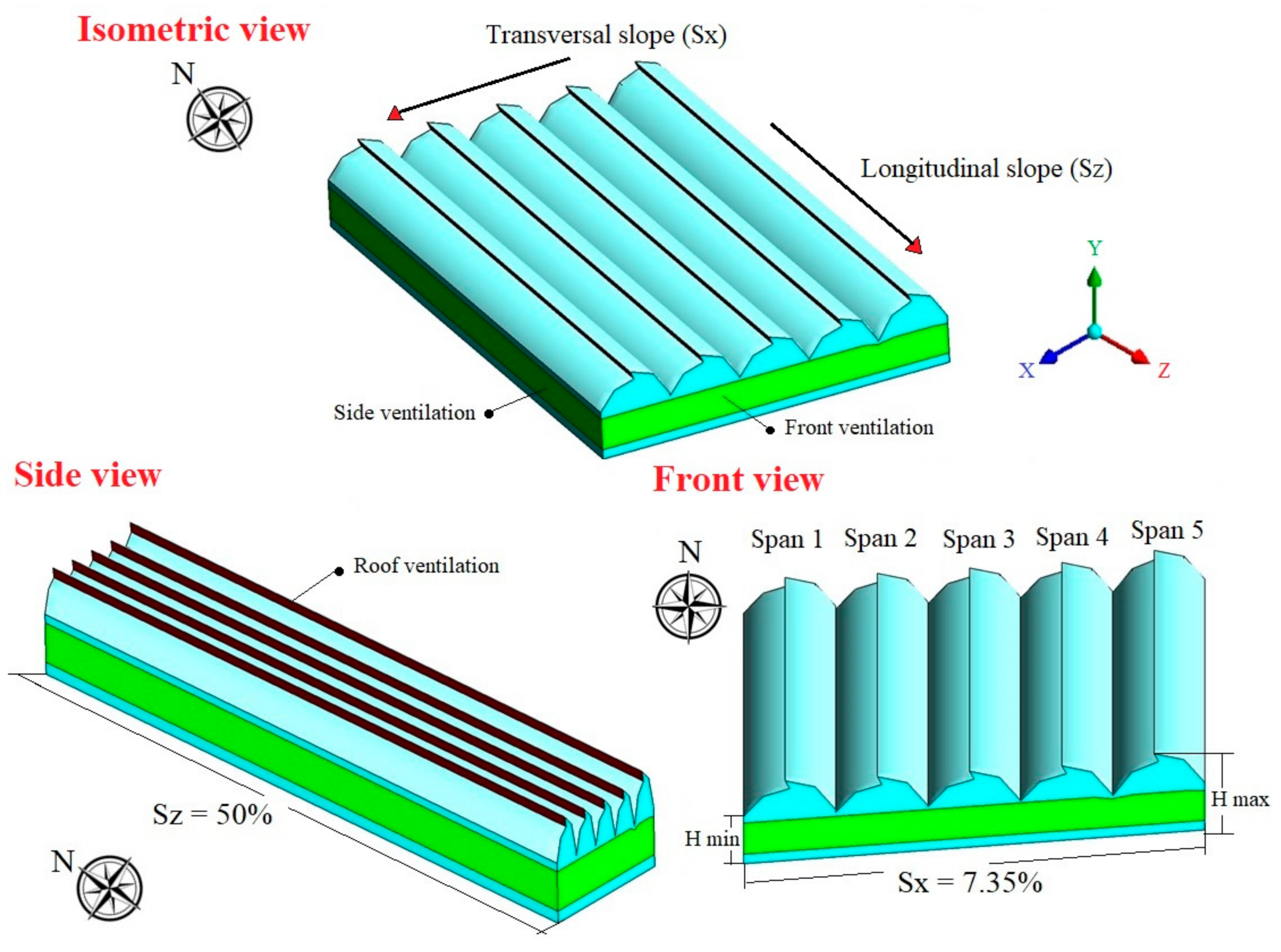
2.1. Description of the Greenhouse and Experimental Site

The greenhouse evaluated in this study is of the multitunnel type with a plastic cover, composed of five adjoining spans, with the width of each span being 6.8 m. Therefore, the total width of the greenhouse is 34 m (X-axis). The longitudinal dimension of the greenhouse is 30 m (Z-axis), the greenhouse has a minimum height above the gutter of 3.5 m (H_min) and a maximum height (H_max) above the ridge of the zenithal ventilation of 5.8 m (Figure 1). The greenhouse has lateral ventilation areas on both sides, with a maximum opening of 2.3 m, so that the ventilation area in the lateral region is 138 m² (13.5% of the covered surface area).

The ventilation surface is complemented by a ventilation area on each of the façades of 2.2 m total opening, giving a total ventilation surface on the façades of 149.6 m² (14.6% of the covered surface area), and finally, each span has a fixed roof ventilation of 0.66 m opening, with the total roof ventilation area being 99 m² (9.7% of the covered surface area) distributed over five spans. The greenhouse was built on a site that had a transversal slope (Sx) of 7.35% and a longitudinal slope (Sz) of 50% (Figure 1).

The experimental site where the greenhouse was located corresponds to the municipality of Filandia (75°42′57.39′′ W, 4°41′11.7′′ N and altitude: 1586 m), in the department of Quindío. This region has a climatic behavior characterized by humid tropical climate conditions, where the average multiannual temperature value for a 35-year period is 20.95 °C and the minimum and maximum mean values are 15.4 °C and 26.6 °C respectively, while the mean annual value of accumulated precipitation is 2060 mm.

2.2. CFD Numerical Model

The numerical solution is developed from the spatial discretization of the nonlinear partial Navier–Stokes equations. The transport phenomena by free convection can be described by Equation (1), which is considered the general transport equation for a fluid in steady state in a three-dimensional field of action.

$$\frac{\partial \left(u\varnothing \right)}{\partial x}+\frac{\partial \left(v\varnothing \right)}{\partial y}+\frac{\partial \left(w\varnothing \right)}{\partial z}=\mathsf{\Gamma }{\nabla }^2\varnothing +S_{\varnothing }$$

(1)

where y, x and z represent the coordinates in Cartesian space, u, v and w are the components of the velocity vector, ${\nabla }^2$ is the Laplacian operator, $\mathsf{\Gamma }$ is the diffusion coefficient, $\varnothing$ represents the concentration of the transported quantity in dimensionless form (momentum, mass and energy) and $S_{\varnothing }$ is the source term. The turbulent nature of the air flow was simulated by using the empirical turbulence model k-ε standard, a model that has been extensively validated in studies of natural ventilation of agricultural buildings, showing a good fit of the real airflow behavior with respect to the simulated process [7]. The buoyancy effects of air caused by gravity and air density changes were added to the momentum equation as a source term by the Boussinesq approximation, and this model is represented by Equation (2) [41].

$$\rho ={\rho }_0\left[1-\beta \left(T-T_0\right)\right]$$

(2)

where $\rho$ and ${\rho }_0$ are the density at a given time and the reference density respectively; $\beta$ is the coefficient of thermal expansion of air; $T$ and $T_0$ are the temperature and the reference temperature. The radiation model selected was the discrete ordinate (DO) model with angular discretization. This model allows the calculation of radiation and convective exchanges occurring in the computational domain, treating the greenhouse canopy as a semitransparent medium [42]. Equation (3) describes the DO radiation model.

$$\begin{gathered} \nabla .\left(I_{\lambda }\left(\underset{r}{\Rightarrow }, \underset{s}{\Rightarrow }\right) \underset{s}{\Rightarrow }\right)+\left(a_{\lambda }+{\sigma }_s\right)I_{\lambda }\left(\underset{r}{\Rightarrow }, \underset{s}{\Rightarrow }\right)=a_{\lambda }{n}^2\frac{\sigma T^4}{\pi }+\frac{{\sigma }_s}{4\pi }{{\displaystyle \int }}_0^{4\pi } \\ {I}_{\lambda }\left(\underset{r}{\Rightarrow }, \underset{s}{\Rightarrow }{}^{\prime }\right)\mathsf{\Phi }\left(\underset{s}{\Rightarrow }. \underset{s}{\Rightarrow }{}^{\prime }\right)d{\mathsf{\Omega }}^{\prime } \end{gathered}$$

(3)

where $I_{\mathsf{\lambda }}$ is the intensity of radiation at one wavelength; $\underset{r}{\Rightarrow } \mathrm{and}\underset{s}{\Rightarrow }$ are the vectors that indicate the position and direction, respectively; ${\underset{s}{\Rightarrow }}^{\prime }$ is the dispersion direction vector; ${\sigma }_s\mathrm{and}{a}_{\lambda }$ are the spectral scattering and absorption coefficients; $n$ is the refractive index; $\nabla$ is the divergence operator and $\mathsf{\Phi },\mathrm{T}$ and $\mathsf{\Omega }$ are the phase function, local temperature (°C) and solid angle, respectively. The non-grey model was activated by dividing the radiative spectrum into two specific wavelengths, the first being the solar radiation length (0.4–2.4 µm) and the second the long wavelength (2.4–100 µm).

Likewise, in order to simplify the resolution of the 3D CFD model, no crops were included, in order to speed up the numerical calculation and establish the behavior of air flow and temperature under the worst possible scenario, which are conditions where there are no plants present, a scenario where a large part of the incident radiation on the interior of the greenhouse is converted into heat, which generates an increase in the temperature of the interior air [2].

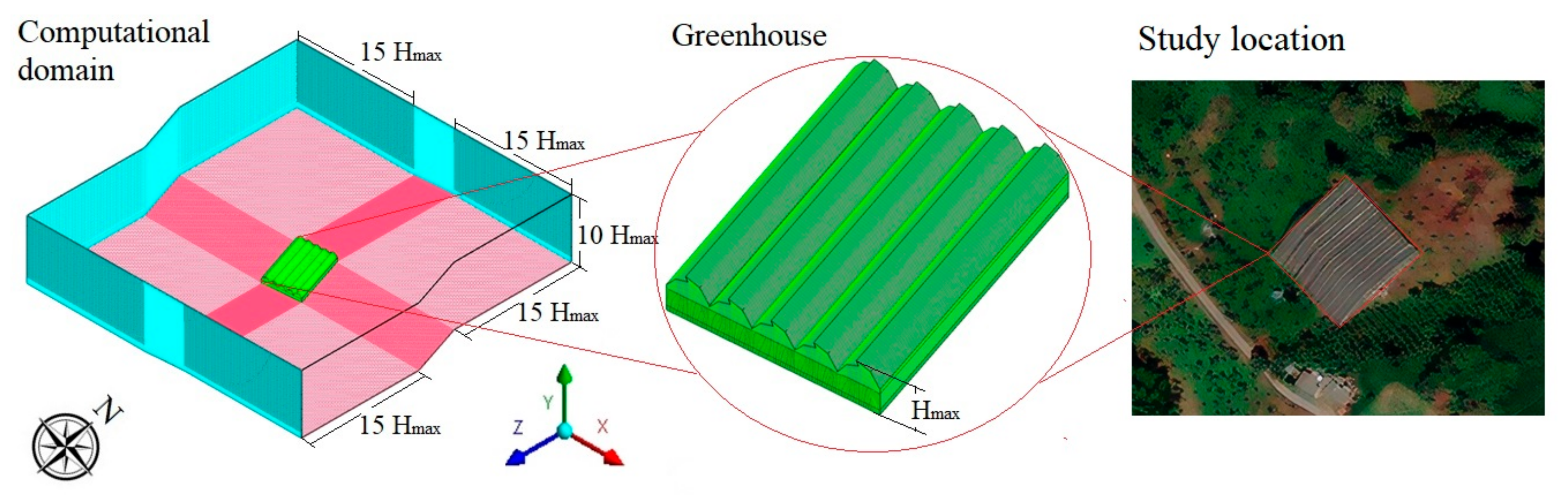
2.3. Discretisation of the Computational Domain

The computational domain that included the greenhouse was configured in terms of its dimensions following the recommendations reported in the work developed by Franke et al. [43] and implemented by Kim et al. [44]. Where minimum lengths are suggested from the edges of the domain to the evaluated structure, these dimensions are established according to the maximum height of the greenhouse (H_max), as shown in Figure 2. Therefore, the overall dimensions of the computational domain for the x, y and z axes were 208 m, 58 m and 204 m respectively.

This computational domain was divided into an unstructured numerical grid with a size determined from a test of independence on the size of the numerical grid. The results obtained in this test will be discussed later in this paper. The quality of the selected numerical grid was determined from the orthogonality parameter, finding that 95.2% of the grid elements had a value higher than 0.93, considered to be of high quality [45]. It should be noted that both the size of the numerical grid and the quality of its elements should be verified by the two methodologies discussed above, since these factors are highly determinant of the quality and accuracy of the numerical results obtained [11].

As for the solver settings, a semi-implicit method was used for the coupling of the pressure–velocity equations using the SIMPLE algorithm. For the momentum, energy, and pressure terms, a second order discretization scheme was used, which allows more accurate results to be obtained compared to the first order discretization schemes [46]. Finally, convergence criteria were established in 10⁻⁶ for the energy equation and in 10⁻³ for the other variables of the model [1]. For the radiation model, we defined the following discretization conditions; 3 theta and phi divisions, 3 theta and phi pixels and 10 energy iterations per radiation iteration.

2.4. Boundary Conditions

In the computational domain, the physical and optical properties of the materials described in

Table 1. Thermophysical and optical properties of computational domain materials.

Property	Soil	Air	Cover Greenhouse	Perimeter Walls
Density (ρ, kg m−3)	1.300	1.023	923	923
Thermal conductivity (k, W m−1 K−1)	1.3	0.0242	0.4	0.4
Specific heat (Cp, J K−1 kg−1)	800	1006.43	2300	2300
Absorptivity	0.90	0.19	0.06	0.93
Scattering coefficient	−15	0	0	0
Refractive index	1.92	1	1.53	1.53
Emissivity	0.95	0.9	0.7	0.7

were used, taking the reference values used in the work carried out by Senhaji et al. [47]. On the other hand, in these 13 simulations a power absorption coefficient ($\alpha \lambda$) was established to obtain a transmittance of zero for long wavelengths and 0.8 for short wavelengths. This can be determined by using Equation (4), which relates the absorptivity ($\alpha$) and the thickness of the medium ($e$).

$$\alpha \lambda =\frac{1}{e}\ln \left(\frac{1}{1-\alpha }\right)$$

(4)

The boundary conditions established were symmetrical for the computational domain boundaries parallel to the air flow. In the case of the greenhouse floor and computational domain, it was simulated as a mixed boundary condition for radiative and convective heat transfer and as an opaque medium for diffuse radiation. On the other hand, the greenhouse roof was simulated as a semitransparent material with a finite thickness of 0.2 mm and a two-sided wall boundary condition and a coupled thermal condition. The greenhouse walls were simulated as an opaque and coupled medium.

In the case of the computational domain roof region, a wall boundary condition was established with a solar radiation flux. A logarithmic input velocity profile was considered at the input of the computational domain. The profile was linked to the main CFD module using the user-defined function (UDF), as explained in the work developed by Villagran et al. [7], using the Equation (5):

$$V_2=V_1\frac{\ln \left(\frac{h_2}{z_0}\right)}{\ln \left(\frac{h_1}{z_0}\right)}$$

(5)

where $V_2$ is the calculated wind velocity in $h_2$ height; $V_1$ is the reported wind velocity in $h_1$ height and $z_0$ is the roughness coefficient length, the surface roughness is a nominal value that depends on the type of coverage and roughness of the soil material, the type of landscape and the spacing between obstacles, for this case was considered a value of 0.03 m in relation to class 1 of roughness according to Bañuelos-Ruedas et al. [48]. In the case of the air flow outlet limit, a pressure outlet limit was established, and, finally, the ventilation areas of the greenhouse were set with an interior condition limit.

2.5. CFD Model Validation and Simulated Scenarios

The CFD model generated was validated through experimental tests inside the greenhouse, with this experimental phase being carried out during the period between 9 February and 12 August 2018, and included the measurement and recording of the main climatic variables of the in the external environment of the greenhouse, such as wind speed (range: 0–89 ms⁻¹, resolution: 0.1 ms⁻¹, accuracy: ±5%), wind direction (range: 0–359°, resolution: 1.0°, accuracy: ±3%), solar radiation (range: 0–1800 Wm⁻², resolution: 1 W m⁻², accuracy: ±5%), temperature (range: −(40)–60 °C, resolution: 0.1 °C, accuracy: ±2%) and air humidity (range: 1–100%, resolution: 1%, accuracy: ±2%), by means of a Vantage Pro 2 weather station (Davis Instruments, Hayward, CA, USA).

Likewise, for the recording of the temperature inside the structure over the longitudinal middle region (Z-axis = 15 m) and over a cross section of the structure and a height of 1.5 m above ground level were installed 7 thermocouples (range:−(40)–70 °C, resolution: 0.1 °C, accuracy: ± 0.3 °C) coupled to a data logger (Cox-Tracer Junior, Escort DLS, Edison, NJ, USA). While 3 sonic anemometers (Mod. WindMaster 3D Anemometer, Gill Instrument Ltd., Hampshire, UK; range: 0–50 ms⁻¹ and 0–359°, resolution: 0.01 ms⁻¹ and 0.1°) were installed for wind speed registration (Figure 3).

With the climatic information collected during the experimental period, the average values of temperature, solar radiation, wind speed and direction were calculated on an hourly scale. These values were used as initial conditions to perform 13 steady-state simulations for each of the hours of the day between 6:00 and 18:00 h, as shown in

Table 2. Initial simulation conditions for each scenario studied.

Hour	Solar Radiation (Wm−2)	Temperature (°C)	Wind Velocity (ms−1)	Wind Direction
6:00	34.3	16.7	0.32	S
7:00	69.2	17.6	0.41	S
8:00	93.7	19.1	0.51	SS
9:00	183.5	20.9	0.65	S
10:00	321.9	22.3	0.91	WSW
11:00	456.6	22.9	1.19	W
12:00	612.4	24.5	1.23	W
13:00	780.1	25.3	1.24	W
14:00	657.2	25.5	1.29	SSW
15:00	312.1	23.4	0.91	SSW
16:00	276.1	21.9	0.62	S
17:00	98.1	20.3	0.66	S
18:00	31.5	19.4	0.53	S

. The value of the wind speed outside corresponds to the value of the reference speed ($V_1$) in Equation (5).

To evaluate the validity of the numerical model, once the hourly simulations had been carried out, the temperature and wind speed data were extracted for each sampling point inside the greenhouse. In a first analysis, the validity or rejection of the numerical simulation model was checked through a statistical analysis by means of a hypothesis test for the difference of measurements with homogeneous variances. In a subsequent step, the simulated data were compared with the measured data through goodness-of-fit parameters such as mean absolute error (MAE) Equation (6) and root mean square error (RMSE) Equation (7).

$$\mathrm{MAE}=\frac{1}{M}{\displaystyle \sum }_{j=1}^M\left|Dmj-Dsj\right|$$

(6)

$$\mathrm{RMSE}=\sqrt{{{\displaystyle \sum }}_{j=1}^M\frac{{\left|D{m}_i-D{s}_i\right|}^2}{M}}$$

(7)

where $D{m}_j \mathrm{and}D{s}_j$ are the measured and simulated wind speed and temperature values at point j respectively and M is the number of samples. Once the CFD model was validated, we proceeded to the post-processing phase where air flow behavior curves were extracted from the numerical solution. In this case, inside the greenhouse in a plane (z, x) at a height (y) of 1.5 m above the ground level, a total set of 18,951 spatial data were extracted for temperature and wind speed; data that will be analyzed in the results section.

In this post-processing phase, the data for the calculation of the ventilation rate are also extracted. This process is performed by the conventional method that consists of verifying the greenhouse outflows at each ventilation opening. Therefore, the greenhouse air exchange rate (GAER) per unit time in minutes is calculated by Equation (8).

$$\mathrm{GAER}=\frac{\sum V_i\ast A_{vs}}{V_G}\ast 60$$

(8)

where $V_i$ is the air velocity of the outflow (ms⁻¹), $A_{vs}$ is the area of the ventilation with exhaust air flow (m²) and $V_G$ is the volume of the greenhouse (m³).

3. Results and Discussion

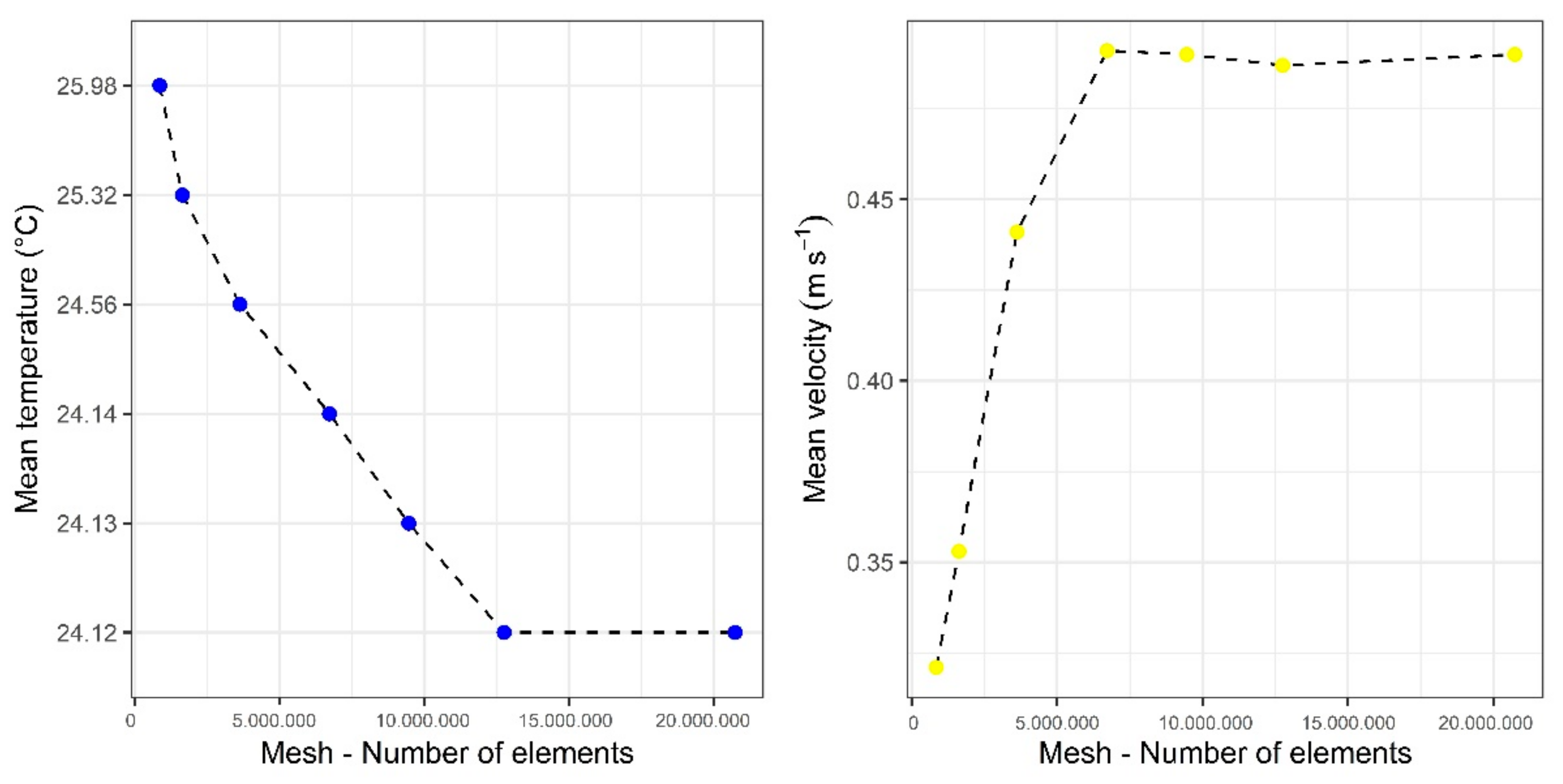
3.1. Grid Independence Test

For the grid independence test, the mean values calculated for hour 10 were selected as initial conditions (Table 2). With these values, eight simulations were performed, where the variable of change was the number of elements of the numerical grid, for which a total of eight grids of different sizes were available. These grids varied between a minimum of 846,819 elements for grid 1 and a maximum of 20,735,202 elements for grid 7.

For this case, grid number 4 was selected, which is made up of a total number of 6,717,534 elements. This selection was made because quantitatively it was possible to verify that from this grid size the solutions obtained for temperature and velocity are independent of the number of elements that make up the numerical grid, as can be seen graphically in Figure 4. This independence test should always be performed in CFD studies since its results can be used to define the numerical grid size that guarantees the independence and accuracy of the solutions at the lowest possible computational cost [49,50].

3.2. Data and Validation of CFD Model

The air velocity values obtained under experimental and simulated conditions at each of the three measurement points, for each of the 13 scenarios evaluated (6:00–18:00 h) can be found in

Table 3. Experimental and simulated values of air velocity for each scenario.

Hour	Sensor	MAV * (ms−1)	SAV * (ms−1)	Hour	Sensor	MAV * (ms−1)	SAV * (ms−1)	Hour	Sensor	MAV * (ms−1)	SAV * (ms−1)
6:00	1	0.34	0.39	11:00	1	0.83	0.79	16:00	1	0.97	1.03
6:00	2	0.42	0.43	11:00	2	0.85	0.83	16:00	2	0.95	1.00
6:00	3	0.37	0.36	11:00	3	0.90	1.00	16:00	3	1.04	1.13
7:00	1	0.50	0.47	12:00	1	1.12	0.98	17:00	1	0.89	0.90
7:00	2	0.48	0.47	12:00	2	1.10	0.93	17:00	2	0.78	0.82
7:00	3	0.44	0.43	12:00	3	1.12	1.13	17:00	3	0.7	0.72
8:00	1	0.49	0.53	13:00	1	1.05	1.02	18:00	1	0.61	0.51
8:00	2	0.61	0.59	13:00	2	1.02	0.99	18:00	2	0.60	0.52
8:00	3	0.62	0.64	13:00	3	1.14	1.25	18:00	3	0.54	0.41
9:00	1	0.71	0.67	14:00	1	1.15	1.11
9:00	2	0.81	0.76	14:00	2	1.16	1.10
9:00	3	0.87	0.87	14:00	3	1.19	1.18
10:00	1	0.70	0.70	15:00	1	1.02	1.07
10:00	2	0.75	0.77	15:00	2	0.89	0.98
10:00	3	0.73	0.74	15:00	3	1.23	1.28

M_AV * (Measured air velocity); S_AV * (Simulated air velocity).

. The same values obtained for the seven sampling points were obtained for temperature and are summarized in

Table 4. Experimental and simulated values of temperature for each scenario.

Hour	Sensor	MT * (°C)	ST * (°C)	Hour	Sensor	MT * (°C)	ST * (°C)	Hour	Sensor	MT * (°C)	ST * (°C)	Hour	Sensor	MT * (°C)	ST * (°C)
6:00	1	16.8	16.7	10:00	1	23.0	22.5	14:00	1	26.2	26.0	18:00	1	20.1	19.5
6:00	2	16.9	17.1	10:00	2	23.2	22.9	14:00	2	26.7	26.9	18:00	2	19.9	19.8
6:00	3	16.9	17.0	10:00	3	24.1	23.8	14:00	3	27.8	27.8	18:00	3	19.8	19.7
6:00	4	17.0	17.2	10:00	4	24.6	24.7	14:00	4	29.2	28.8	18:00	4	19.9	19.7
6:00	5	17.1	17.2	10:00	5	24.6	24.3	14:00	5	29.2	28.8	18:00	5	20.0	19.8
6:00	6	17.1	17.1	10:00	6	24.5	24.2	14:00	6	29.0	28.4	18:00	6	19.8	19.7
6:00	7	16.9	16.7	10:00	7	25.1	25.0	14:00	7	29.0	29.0	18:00	7	19.8	19.6
7:00	1	17.8	17.7	11:00	1	23.3	23.1	15:00	1	24.2	24.2
7:00	2	18.2	18.2	11:00	2	23.7	23.6	15:00	2	24.8	25.0
7:00	3	18.3	18.2	11:00	3	24.4	24.5	15:00	3	25.9	25.6
7:00	4	18.6	18.4	11:00	4	25.3	25.6	15:00	4	26.2	26.0
7:00	5	18.7	18.5	11:00	5	26.6	26.5	15:00	5	26.1	25.9
7:00	6	18.4	18.2	11:00	6	25.7	25.6	15:00	6	26.1	25.7
7:00	7	18.1	17.7	11:00	7	26.0	26.2	15:00	7	26.0	26.4
8:00	1	19.5	19.4	12:00	1	24.9	24.7	16:00	1	22.5	22.3
8:00	2	20.2	19.9	12:00	2	25.1	24.9	16:00	2	23.8	24.0
8:00	3	20.4	20.0	12:00	3	26.2	25.8	16:00	3	23.7	23.6
8:00	4	20.4	20.3	12:00	4	27.4	27.2	16:00	4	24.1	24.2
8:00	5	20.8	20.4	12:00	5	28.7	28.3	16:00	5	24.1	24.0
8:00	6	20.8	20.5	12:00	6	28.3	28.2	16:00	6	24.3	24.5
8:00	7	19.9	19.4	12:00	7	28.9	28.4	16:00	7	23.2	22.4
9:00	1	21.2	21.3	13:00	1	25.4	25.5	17:00	1	21.0	20.9
9:00	2	22.3	22.1	13:00	2	26.1	25.8	17:00	2	21.9	22.0
9:00	3	22.5	22.3	13:00	3	26.5	26.9	17:00	3	21.8	21.5
9:00	4	22.9	22.7	13:00	4	27.9	28.6	17:00	4	22.0	21.9
9:00	5	23.0	23.0	13:00	5	29.4	29.9	17:00	5	21.9	21.9
9:00	6	23.4	23.1	13:00	6	29.4	29.6	17:00	6	21.8	21.7
9:00	7	22.3	21.3	13:00	7	29.8	30.0	17:00	7	21.5	20.9

M_T * (Measured temperature); S_T * (Simulated temperature).

. These values were the data used to perform the validation process of the CFD model.

Table 5. Results of the test statistics of the data obtained using the CFD model.

F Test to Compare Two Variances	H0: σ(Dm)2 = σ(Ds)2  o  H1: σ(Dm)2 ≠ σ(Ds)2
	Temperature	Air Velocity
F	0.9787	0.926
p-value	0.919	0.815
95% confidence interval.	[0.646, 1.483]	[0.486, 1.767]
Two sample t-test	H0: µDm = µDs  o  H1: µDm ≠ µDs
	Temperature	Air velocity
t	0.238	0.053
p-value	0.811	0.957
95% confidence interval.	[−0.928, 1.184]	[0.114, 0.121]

shows the results obtained for both air velocity and temperature from the homogeneity of variances tests and the respective mean comparison test between measured and simulated data. In general, it was found that there were no significant differences between the variances of the simulated and measured data for temperature and air velocity at a 95% interval, and likewise, no statistically significant differences were observed between these sets of measured and simulated data at a 95% confidence interval for the difference in means. In all these statistical tests, the null hypothesis (H₀) is accepted.

Figure 5 shows the behavior of the measured and simulated data for the temperature variable, over the experimentally studied cross section. In general terms, it can be observed that the data sets for the spatial points sampled show very similar behavior in terms of magnitude and trend in the totality of the hours evaluated. This analysis was complemented with the numerical analysis based on the goodness-of-fit criteria selected, the results of which are shown in

Table 6. Values of the goodness-of-fit parameters obtained for temperature and air velocity.

Hour	Temperature		Air Velocity
	MAE (°C)	RMSE (°C)	MAE (ms−1)	RMSE (ms−1)
6:00	0.124	0.140	0.025	0.032
7:00	0.165	0.195	0.014	0.016
8:00	0.309	0.336	0.024	0.026
9:00	0.289	0.429	0.030	0.037
10:00	0.267	0.295	0.010	0.012
11:00	0.153	0.169	0.052	0.062
12:00	0.274	0.300	0.107	0.128
13:00	0.345	0.397	0.054	0.065
14:00	0.269	0.336	0.035	0.040
15:00	0.242	0.267	0.065	0.068
16:00	0.266	0.354	0.070	0.072
17:00	0.186	0.262	0.029	0.030
18:00	0.218	0.267	0.096	0.097

.

For the temperature variable, it was found that the MAE value oscillated between minimum and maximum values of 0.124 °C and 0.346 °C for 6:00 and 13:00 h respectively, while the RMSE values oscillated between 0.140 and 0.397 °C for these same hours. These values found are within the ranges reported in previous studies where CFD models were implemented to determine airflow patterns and thermal distribution in naturally ventilated greenhouses [34,51].

In the case of the air velocity variable inside the greenhouse evaluated, the spatial distribution of the measured and simulated values for each hour was plotted, finding that the experimentally sampled values showed high coincidence with the simulated values (Figure 6). Likewise, the results of the quantitative analysis of the measured and simulated data sets through MAE and RMSE (Table 6) showed values lower than 0.107 ms⁻¹ and 0.128 ms⁻¹ respectively, values that can be considered highly acceptable for these types of modelling and simulation study [7,12]. Therefore, under this quantitative and qualitative analysis of the temperature and wind velocity data, it can be concluded that the numerical model has a high capacity for the prediction of the air flow patterns and the spatial distribution of temperature in the greenhouse studied.

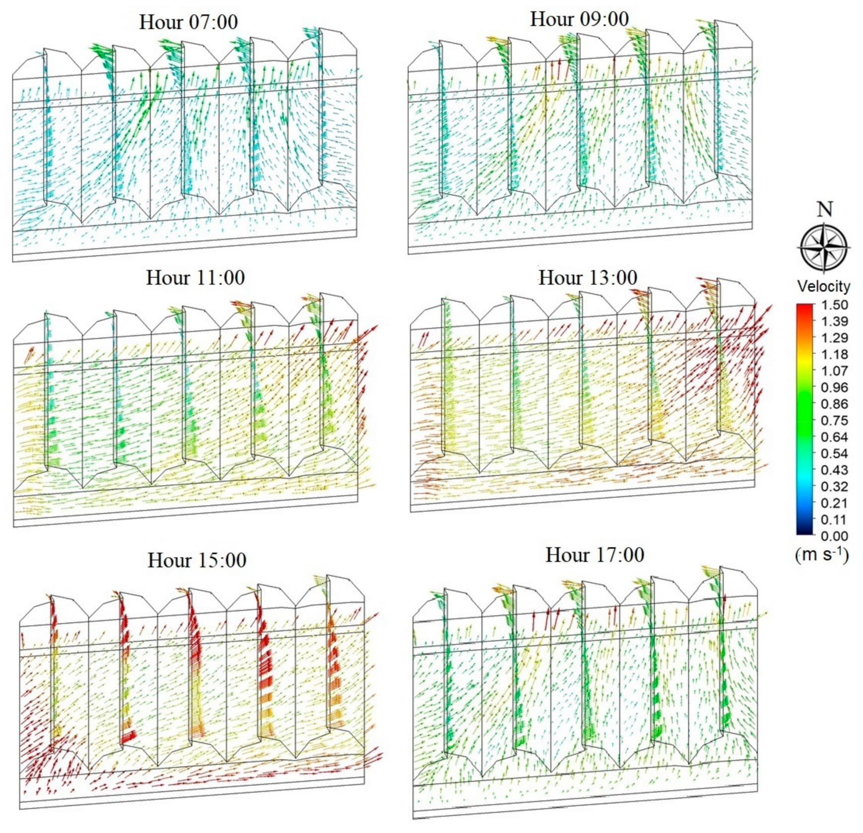
3.3. Qualitative and Quantitative Characteristics of Airflow Patterns

The airflow patterns inside the greenhouse for some of the simulated scenarios are shown in Figure 7. For the 07:00 and 09:00 h where the wind comes from the south side, air flow patterns were observed entering the greenhouse through the side vents and the ventilation area of the façade exposed to windward, with these air flows moving in the longitudinal direction of the greenhouse ascending the slope of the land, until they leave the interior of the structure through the ventilation area located on the north façade of the greenhouse.

It is also observed that in spans 3, 4 and 5 the airflow patterns enter with a low velocity of approximately 0.23 ms⁻¹, and then accelerate to a velocity of 0.67 ms⁻¹ as these airflows ascend the slope of the terrain. This acceleration of the airflow may be influenced by the convective effect caused by changes in density as a function of the change in temperature of the air inside the structure [47].

It is also observed that the fixed vents in the roof region for this case function as air inlet areas over a region approximately in the lower 3/4 of the longitudinal section and an air outlet area approximately over the upper 1/4 of the longitudinal section in all the spans. This may indicate that the longitudinal slope generates on the fixed windows of the greenhouse roof regions positive pressure for the air inlet zones and negative pressure for the window section where there is an air outlet flow [52,53].

For the 11:00 and 13:00 h, a change in the air flow pattern inside the greenhouse is observed, mainly influenced by the direction of the dominant outside wind, which in this case comes from the west side of the greenhouse. Therefore, the airflows enter the greenhouse through the windward side ventilation with average velocities of 1.07 ms⁻¹ and 1.19 ms⁻¹ for each case. Between spans 1 and 2 these airflows presented a deceleration and again from span 3 to span 5 they accelerated until they reached and exceeded the entry velocity values (Figure 7).

The air flows inside the greenhouse moved in two identifiable patterns (Figure 7, hour 11:00 and 13:00). The first moved close to the lower façade of the greenhouse and as it crossed the cross section it moved in the opposite direction to the longitudinal slope until it exited completely through the leeward side vent. The other flow moved through the greenhouse in a counter-slope direction and exited the structure through the façade located on the north side (Figure 7, hour 11:00 and 13:00). In these scenarios a flow pattern was again identified in the fixed roof windows similar to the one already discussed in the two previous scenarios.

In the case of 15:00 h, where the wind comes from the south-southwest side, the airflow entered through the lateral side of the west side and through the windward façade. This air flow then adopted a very similar behavior to that at 13:00 h with the only difference being that in this case a higher velocity (1.29 ms⁻¹) was observed in the entry of the air flow into the structure and in turn a higher velocity in the fixed roof ventilation areas (between 1.18 and 1.39 ms⁻¹).

Finally, for the 17:00 h scenario, the same characteristic pattern already discussed for the 07:00 and 09:00 h scenarios are observed. Within these results it can be observed that the variables have already been discussed in previous works where it was defined that the air flow patterns are influenced by the shape, height and size of the greenhouse, the geometry of the roof, the arrangement of windows, and the speed and direction of the outside air flow [6,11,54]. The topography of the terrain where the greenhouse is built must be added, since this factor also influences the behavior of the air flows, both in their direction of displacement and in their velocity value.

The presence of longitudinal and transverse slopes on the ground influences the air flow patterns since these slopes favor a behavior where air flows lose velocity once they enter the greenhouse and in turn the air flow pattern tends to be directed vertically towards the roof ventilation areas while moving in a counter-slope direction. This type of flow pattern had already been reported in the study developed by Taloub et al. [55], who concluded that any type of slope on the floor of the greenhouse, no matter how small, destabilizes the horizontal airflow and promotes the generation of vertical airflows and recirculatory movement patterns with low velocity zones near the leeward vents.

3.4. Air Velocity Inside the Greenhouse and Calculated Ventilation Rates

The average air velocity values and their standard deviation for each of the evaluated scenarios are shown in Table 4. In general terms, the average air flow velocity in the greenhouse ranged from a minimum of 0.312 ± 0.08 ms⁻¹ at 06:00 h to a maximum of 1.336 ± 0.29 ms⁻¹ at 15:00 h. The average velocities found for this greenhouse were higher than those reported for other greenhouses studied under the conjugated ventilation configuration with side and roof ventilation areas, where the value reported in several studies ranged between 0.5 and 0.7 ms⁻¹ [56,57,58]. This behavior may be highly influenced by the slopes of the land where the greenhouse was built, and also by the lack of insect netting in the ventilation areas, since in Colombia the use of insect netting is not a common practice.

On the other hand, the behavior of the normalized velocity, which represents the relationship between the average inside air velocity and the outside wind speed, showed a minimum and maximum of 83.1% and 146.8%, respectively (

Table 7. Air velocity values obtained inside the greenhouse for each simulated scenario.

Hour	Average Air Velocity (ms−1)	Normalized Air Velocity (%)
6:00	0.312 ± 0.08	97.1
7:00	0.404 ± 0.10	98.5
8:00	0.505 ± 0.12	99.1
9:00	0.641 ± 0.15	98.6
10:00	0.871 ± 0.14	95.7
11:00	0.989 ± 0.15	83.1
12:00	1.129 ± 0.16	91.8
13:00	1.191 ± 0.18	96.7
14:00	1.269 ± 0.20	98.3
15:00	1.336 ± 0.29	146.8
16:00	0.819 ± 0.17	132.1
17:00	0.812 ± 0.14	123.1
18:00	0.565 ± 0.10	106.7

). These values of normalized velocity, contrary to other studies of natural ventilation, were relatively high, which is influenced by the acceleration of the air flow inside the greenhouse. It was also found that for the period between 15:00 and 18:00 h, the value of the normalized velocity was higher than 100%, which means that the air flow velocity inside the structure was higher than the external wind flow.

The values of the highest normalized velocity agreed with the time when the temperature of the outside environment started to decrease, therefore it can be mentioned that this acceleration of the air flow inside the greenhouse may be strongly associated with the thermal effect of natural ventilation by buoyancy; an effect that generally produces rapid changes in temperature and velocity inside a greenhouse [59]. This buoyancy phenomenon is caused by convective movements generated between the soil and the greenhouse cover, since at that time the soil is the surface of higher temperature due to energy storage throughout the day, while the cover usually cools rapidly to the level of the outside ambient temperature [34,60].

This type of behavior analyzed serves as a basis for generating a recommendation for management and microclimatic optimization for night-time hours in these structures that do not have opening and closing systems for side and roof vents. A useful alternative to prevent the accelerated loss of stored heat during the hours of high temperature and solar radiation would be the use of a mechanism to close the ventilation areas just around 15:00 h, which is the time when the ambient temperature begins to decrease. Therefore, a mechanism to close each of the side and roof vents would increase the hermeticity of the greenhouse and prevent thermal inversion phenomena during nighttime hours [50,61,62].

Greenhouse air exchange rates (GAERs) in volumes per minute (Vmin⁻¹) were calculated for each of the simulated hours, with these values ranging between a minimum and maximum value of 0.28 Vmin⁻¹ and 1.29 Vmin⁻¹ (Figure 8). These data show that only for a period of 3 h (12:00–15:00) was the GAER value higher than the minimum recommended value for passive greenhouses, which should be at least 1 volume renewed per minute (Vmin⁻¹) [59]. Therefore, it can be deduced that the greenhouse evaluated presents deficient ventilation rates for 69.7% of the hours of the day-time period, and so it is recommended that future studies address design alternatives in the structure to maximize this index, since its influence on the microclimate behavior of the structure is very relevant [63].

In general terms, it can be observed that as the day went by 6:00–14:00 h and at the same time there was an increase in the outdoor wind speed, there was an increase in the value of the air exchange rate of the greenhouse (Figure 8). Therefore, for the period between 6:00 and 14:00 h, the GAER value increased from 0.28 to 1.23 Vmin⁻¹, which represents an increase of 331% between 6:00 and 14:00 respectively. For this same period, the wind speed had an increase of 303%, increasing from a value of 0.32 ms⁻¹ at 6:00 to a value of 1.29 ms⁻¹ at 14:00 (Figure 8).

The above reaffirms what has already been reported in other studies of natural ventilation, where it was identified that there is a direct relationship between the ventilation rate and the outside air flow velocity [8,64]. Figure 9 shows the linear relationship between GAER (y) and the external wind speed (x), which can be represented mathematically with the equation Y = 1.0291 (X) − 0.1099, which in this case is a relationship with an acceptable coefficient of determination R² of 0.8085.

3.5. Qualitative and Quantitative Characteristics of the Spatial Distribution of Temperature

The spatial distribution of temperature for each of the simulated scenarios can be seen in Figure 10. The behavior found shows the thermal gain that occurs in the structure via the greenhouse effect between 6:00 and 14:00 h, where the volume of air enclosed inside the structure is heated by the combined effect of higher values of solar radiation and the increase in temperature in the outside environment, which is a typical behavior of structures at the tropical level [65].

Subsequently, from 15:00 to 18:00 h, a totally opposite phenomenon is observed, where an accelerated cooling of the air volume occurs due to the reduction of the temperature and radiation levels in the external environment. This heat loss is more accelerated in this structure since it does not have enclosure systems that limit the air flow through the lateral and roof ventilation areas.

Another characteristic observed is the spatial heterogeneity in the value of the temperature presented in this type of greenhouse. For the first hours of the day some zones of higher temperature are observed just below the areas covered by spans 2, 3 and 4, and this same behavior is observed for the hour 17:00 (Figure 10), while for 11:00, 13:00 and 15:00 a zone of higher temperature is observed in the region below spans 4 and 5.

Another aspect to be highlighted is the influence of the wind direction on the location of the high temperature zones. For the cases where the wind direction comes from the south, the region of higher temperature is concentrated from the middle longitudinal zone of the greenhouse towards the leeward façade, hours 7:00, 9:00 and 17:00 (Figure 10). For the hours 11:00, 13:00 and 15:00, however, where the outside wind comes from the west, the warm regions are located on the leeward side and on the area near the north façade just below spans 3, 4 and 5 (Figure 10).

Qualitatively, it can be observed on the spatial distribution patterns of temperature for each evaluated scenario that tends to generate a zone with higher temperature values just above the regions of higher altitude in the greenhouse, these are areas that in our case are located near the north facade and the top of the east side of the structure. These regions of higher temperature located in the upper slopes of the terrain were reported in a Costa Rica greenhouse evaluated in the work developed by Rojas Rishor [38], who also reported these same heat patches even with the outside airflow moving downslope. Therefore, it is important to recommend that developers building on slopes should monitor and establish cooling strategies in the higher altitude regions of the terrain.

3.6. Temporal Behavior of the Temperature Inside the Greenhouse

Temperature is one of the main microclimate variables directly involved in the growth and development of most crops of commercial and food interest, and this variable also affects the photosynthetic activity of the plant and the quality of the final product. For this reason it is one of the most studied microclimate variables inside greenhouses [63,66].

The qualitative analysis of the spatial temperature patterns was performed by calculating the average values of the temperature inside the greenhouse (T_inside) and the thermal gradient generated inside the structure (ΔT_inside). This gradient represents the difference between the maximum temperature (T_max) and the minimum temperature (T_min) in the indoor environment for each of the hours (

Table 8. Values obtained for T_inside and ΔTi_nside in each simulated scenario.

Hour	Tinside	ΔTinside = Tmax − Tmin
6:00	16.98 ± 0.28	1.55
7:00	18.12 ± 0.42	2.15
8:00	19.91 ± 0.55	3.05
9:00	22.13 ± 0.92	4.84
10:00	23.88 ± 1.21	8.50
11:00	24.87 ± 1.50	11.18
12:00	26.66 ± 1.82	13.15
13:00	27.91 ± 2.19	16.93
14:00	27.92 ± 1.75	11.22
15:00	25.47 ± 1.13	7.90
16:00	23.41 ± 1.19	8.45
17:00	21.62 ± 0.82	5.09
18:00	19.70 ± 0.19	1.26

).

The values of Ti_nside ranged between a minimum value of 16.98 ± 0.28 °C for the 6:00 h and a maximum value of 27.92 ± 1.75 °C for the 14:00 h. Between these times it was observed that the greenhouse temperature was gradually increasing, and this type of behavior is very characteristic of greenhouses located in the tropics. Once the highest T_inside value was achieved at about 14:00 h, this value decreased again to a value of 19.70 ± 0.19 °C. Therefore, the greenhouse presented a thermal gain of 10.94 °C in a period of 9 h and an energy loss of 8.22 °C in only 4 h, demonstrating numerically what has already been analyzed qualitatively in the previous section in reference to the accelerated energy loss of this greenhouse.

The values of T_inside found for this structure are within the ranges reported as adequate for most of the species of food/fruit interest such as tomato, cucumber and pepper, additionally, at no time of the day does the temperature exceed the maximum recommended for these types of crop, which is around 35 °C [5,67]. Another factor related to the behavior of temperature is its spatial distribution. In recent years, the interest of researchers has focused on determining and studying the heterogeneous distribution of temperature inside greenhouses, since it is a factor that affects the quantity and quality of the final products harvested [68,69,70].

Regarding the evaluation of the spatial distribution of the temperature, it can be observed that there are behaviors that can be considered as homogeneous for the hours 6:00 and 17:00 where the ΔT_inside value showed values lower than 2 °C [70]. For the remaining hours, a high thermal heterogeneity is observed between 9:00 and 16:00 h, where the ΔT_inside value reached a magnitude of up to 16.93 °C at 13:00 h. This value may be considered too high and inadequate, even more so if we take into account that it is a greenhouse composed of only five spans and that additionally it does not have porous insect-proof mesh protection in the ventilation areas.

This behavior is not ideal for this type of structure since the plants are subjected to different internal temperature conditions for the same external climatic conditions, which generates non-uniform growth and production of crops. The above has a particular aggravating factor, and that is the fact that for these greenhouses, cultural tasks such as irrigation and fertilization were calculated and applied in the same way and quantity for all plants.

On the other hand, the thermal differential between the outdoor and indoor environments (TD = T_outside-T_inside) was calculated, where mean values ranging from 0.28 °C for 6:00 h to a maximum value of 2.61 °C for 13:00 h were obtained (Figure 11). The figure shows that both the TD thermal gradient and the climatic heterogeneity are dependent on the level of solar radiation; therefore, the higher the radiation levels, the greater the thermal gradients and spatial variability of the temperature inside the greenhouse. These results are consistent with those reported in previous studies of the microclimatic behavior of Colombian greenhouses [65,70,71].

Finally, it is important to mention that the results obtained in this research are a relevant technical input that will allow future microclimatic optimization strategies to manage the temperature conditions inside roof structures built on slope soil. Thermal heterogeneity inside this type of structure is an undesirable condition that puts at risk the sustainability of agricultural production in the future year, considering the increase of temperatures due to climate change as a serious threat in the tropical region [1,2].

Therefore, it is necessary that future studies consider the search for alternatives that allow the management of radiation and temperature in such structures. Currently there are several studies where the use of passive methods has been used to optimize or increase the degree of management of the microclimate in passive greenhouses [1,2]. These passive methods include the management of the radiation level inside the structure through the use of shading nets. The use of shading nets reduces the temperature inside the greenhouse, improves the distribution of climatic parameters such as temperature and relative humidity, and additionally helps to reduce the water consumption of the plants and improve the quality of the final products [72].

It is also possible to contemplate the use of solar panels on the region of the roof where the greatest thermal heterogeneity is generated. This would reduce the temperature value and additionally obtain an energy benefit through the collection of solar energy that can be used for other daily tasks on the farm. This has also showed in several studies that this alternative is economically and technically feasible, although it must always be accompanied by studies that allow establishing the optimal level of shade that does not negatively affect the yield and quality of the crops [73,74].

Another alternative that can be analyzed is the use of bedrock storage systems and water bags as proposed by Gourdo et al. [75] and Bazgaou et al. [76], who reported temperature reductions in a plastic-covered greenhouse between 3 and 5 °C in the daytime hours of the day period. Finally, the CFD model validated in this research can also be used to simulate unbuilt scenarios that modify the current structure and ventilation configuration of this greenhouse, trying to improve the movement of air flow patterns and the spatial distribution of temperature following the methodological approach developed in several studies of natural ventilation in greenhouses that seek to optimize the generated microclimate [5,7,34,77,78].

4. Conclusions

The experimental validity of the 3D CFD model analyzed by means of trend curves and numerical parameters of goodness-of-fit between measured and simulated data exhibited high agreement. Therefore, the numerical model implemented in this research showed a high level of prediction of the air flow patterns and the spatial distribution of temperature generated inside a Colombian greenhouse established on slope soil.

This study identified that the greenhouse evaluated under the current ventilation configuration does not comply with the minimum ventilation rates recommended for a naturally ventilated greenhouse, for 69.7% of the hours evaluated. This generates a spatial distribution of temperature that reaches differences of up to 16.93 °C between the highest and lowest temperatures. These conditions are considered highly heterogeneous and will certainly affect the growth of the crops in this type of greenhouse.

Although the behavior of natural ventilation and the spatial distribution obtained for this greenhouse showed direct relationships with wind speed and the level of solar radiation of the external environment, it was observed that the slope of the terrain affects the displacement and speed of air flows, which generates high temperature zones on the higher regions of the terrain.

Finally, this study can be the baseline for future research aimed at evaluating alternatives to optimize the microclimatic performance of this type of greenhouse built on sloping terrain, since there is currently limited available information for greenhouses under these construction conditions. The validated CFD model can also be implemented for the study of the microclimatic behavior of other types of greenhouses built in Latin American or Caribbean countries, where protected crops are increasingly implemented in soils with slope conditions.

References

1. Villagran, E.; Ramirez, R.; Rodriguez, A.; Pacheco, R.L.; Jaramillo, J. Simulation of the thermal and aerodynamic behavior of an established screenhouse under warm tropical climate conditions: A numerical approach. Int. J. Sustain. Dev. Plan. 2020, 15, 487–499. [Google Scholar] [CrossRef]
2. Villagran, E.; Leon, R.; Rodriguez, A.; Jaramillo, J. 3D numerical analysis of the natural ventilation behavior in a Colombian greenhouse established in warm climate conditions. Sustainability 2020, 12, 8101. [Google Scholar] [CrossRef]
3. Hemming, S.; de Zwart, F.; Elings, A.; Petropoulou, A.; Righini, I. Cherry tomato production in intelligent greenhouses-sensors and ai for control of climate, irrigation, crop yield, and quality. Sensors 2020, 20, 6430. [Google Scholar] [CrossRef] [PubMed]
4. McCartney, L.; Orsat, V.; Lefsrud, M.G. An experimental study of the cooling performance and airflow patterns in a model Natural Ventilation Augmented Cooling (NVAC) greenhouse. Biosyst. Eng. 2018, 174, 173–189. [Google Scholar] [CrossRef]
5. Akrami, M.; Javadi, A.A.; Hassanein, M.J.; Farmani, R.; Dibaj, M.; Tabor, G.R.; Negm, A. Study of the effects of vent configuration on mono-span greenhouse ventilation using computational fluid dynamics. Sustainability 2020, 12, 986. [Google Scholar] [CrossRef] [Green Version]
6. Reynafarje, X.; Villagrán, E.A.; Bojacá, C.R.; Gil, R.; Schrevens, E. Simulation and validation of the airflow inside a naturally ventilated greenhouse designed for tropical conditions. Acta Hortic. 2020, 1271, 55–62. [Google Scholar] [CrossRef]
7. Villagrán, E.A.; Romero, E.J.B.; Bojacá, C.R. Transient CFD analysis of the natural ventilation of three types of greenhouses used for agricultural production in a tropical mountain climate. Biosyst. Eng. 2019, 188, 288–304. [Google Scholar] [CrossRef]
8. Parra, J.P.; Baeza, E.; Montero, J.I.; Bailey, B.J. Natural ventilation of parral greenhouses. Biosyst. Eng. 2004, 355–366. [Google Scholar] [CrossRef]
9. Teitel, M.; Montero, J.I.; Baeza, E.J. Greenhouse design: Concepts and trends. Acta Hortic. 2012, 952, 605–620. [Google Scholar] [CrossRef]
10. Bartzanas, T.; Boulard, T.; Kittas, C. Numerical simulation of the airflow and temperature distribution in a tunnel greenhouse equipped with insect-proof screen in the openings. Comput. Electron. Agric. 2002, 34, 207–221. [Google Scholar] [CrossRef]
11. Bournet, P.E.; Boulard, T. Effect of ventilator configuration on the distributed climate of greenhouses: A review of experimental and CFD studies. Comput. Electron. Agric. 2010, 74, 195–217. [Google Scholar] [CrossRef]
12. Benni, S.; Tassinari, P.; Bonora, F.; Barbaresi, A.; Torreggiani, D. Efficacy of greenhouse natural ventilation: Environmental monitoring and CFD simulations of a study case. Energy Build. 2016, 125, 276–286. [Google Scholar] [CrossRef]
13. Molina-Aiz, F.D.; Valera, D.L.; López, A. Airflow at the openings of a naturally ventilated Almería-type greenhouse with insect-proof screens. Acta Hortic. 2011, 893, 545–552. [Google Scholar] [CrossRef]
14. Akrami, M.; Salah, A.H.; Javadi, A.A.; Fath, H.E.; Hassanein, M.J.; Farmani, R.; Negm, A. Towards a Sustainable Greenhouse: Review of Trends and Emerging Practices in Analysing Greenhouse Ventilation Requirements to Sustain Maximum Agricultural Yield. Sustainability 2020, 12, 2794. [Google Scholar] [CrossRef] [Green Version]
15. Hong, S.W.; Lee, I.B.; Hwang, H.S.; Seo, I.H.; Bitog, J.P.; Yoo, J.I. Numerical simulation of ventilation efficiencies of naturally ventilated multi-span greenhouse in Korea. Trans. ASABE 2008, 51, 1417–1432. [Google Scholar] [CrossRef]
16. Baxevanou, C.; Bartzanas, T.; Fidaros, D.; Kittas, C. Solar radiation distribution in a tunnel greenhouse. Acta Hortic. 2008, 801, 855–862. [Google Scholar] [CrossRef]
17. Liu, X.; Li, H.; Li, Y.; Yue, X.; Tian, S.; Li, T. Effect of internal surface structure of the north wall on Chinese solar greenhouse thermal microclimate based on computational fluid dynamics. PLoS ONE 2020, 15, e0231316. [Google Scholar] [CrossRef] [Green Version]
18. Lee, J.H. Optimization of indoor climate conditioning with passive and active methods using GA and CFD. Build. Environ. 2007, 9, 3333–3340. [Google Scholar] [CrossRef]
19. Jia, Y.; Wang, C.; Zhang, C.; Li, W. Numerical Modelling of Radiation-Convection Coupling of Greenhouse Using Underfloor Heating. Open J. Fluid Dyn. 2017, 3, 448–461. [Google Scholar] [CrossRef] [Green Version]
20. Ghernaout, B.; Attia, M.E.; Bouabdallah, S.; Driss, Z.; Benali, M.L. Heat and Fluid Flow in an Agricultural Greenhouse. Int. J. Heat Technol. 2020, 3, 92–98. [Google Scholar] [CrossRef]
21. Villagrán, E.A.; Jaramillo, J.E.; León-Pacheco, R.I. Natural ventilation in greenhouse with anti-insect screens evaluated with a computational fluid model. Agron. Mesoam. 2020, 31, 698–717. [Google Scholar] [CrossRef]
22. Zhang, X.; Wang, H.; Zou, Z.; Wang, S. CFD and weighted entropy based simulation and optimisation of Chinese Solar Greenhouse temperature distribution. Biosyst. Eng. 2016, 142, 12–26. [Google Scholar] [CrossRef]
23. Bournet, P.E. Assessing greenhouse climate using CFD: A focus on air humidity issues. Acta Hortic. 2014, 1037, 971–986. [Google Scholar] [CrossRef]
24. Dhiman, M.; Sethi, V.P.; Singh, B.; Sharma, A. CFD analysis of greenhouse heating using flue gas and hot water heat sink pipe networks. Comput. Electron. Agric. 2019, 163, 104853. [Google Scholar] [CrossRef]
25. Flores-Velazquez, J.; Villarreal-Guerrero, F.; Rojano-Aguilar, A.; Schdmith, U. CFD to analyze energy exchange by convection in a closed greenhouse with a pipe heating system. Acta Univ. 2019, 29. [Google Scholar] [CrossRef]
26. Aguilar-Rodriguez, C.; Flores-Velazquez, J.; Ojeda-Bustamante, W.; Rojano, F.; Iñiguez-Covarrubias, M. Valuation of the energy performance of a greenhouse with an electric heater using numerical simulations. Processes 2020, 8, 600. [Google Scholar] [CrossRef]
27. Guo, J.; Liu, Y.; Lü, E. Numerical simulation of temperature decrease in greenhouses with summer water-sprinkling roof. Energies 2019, 12, 2435. [Google Scholar] [CrossRef] [Green Version]
28. Sapounas, A.; Bartzanas, T.; Nikita-Martzopoulou, C.; Kittas, C. Aspects of CFD modelling of a fan and pad evaporative cooling system in greenhouses. Int. J. Vent. 2008, 797, 131–137. [Google Scholar] [CrossRef]
29. Tamimi, E.; Kacira, M.; Choi, C.Y.; An, L. Analysis of microclimate uniformity in a naturally vented greenhouse with a high-pressure fogging system. Trans. ASABE 2013, 1241–1254. [Google Scholar] [CrossRef]
30. Akrami, M.; Mutlum, C.D.; Javadi, A.A.; Salah, A.H.; Fath, H.; Dibaj, M.; Farmani, R.; Mohammed, R.H.; Negm, A. Analysis of inlet configurations on the microclimate conditions of a novel standalone agricultural greenhouse for Egypt using computational fluid dynamics. Sustainability 2021, 13, 1446. [Google Scholar] [CrossRef]
31. Jiao, W.; Liu, Q.; Gao, L.; Liu, K.; Shi, R.; Ta, N. Computational Fluid Dynamics-Based Simulation of Crop Canopy Temperature and Humidity in Double-Film Solar Greenhouse. J. Sens. 2020. [Google Scholar] [CrossRef]
32. Villagran, V. Implementation of ventilation towers in a greenhouse established in low altitude tropical climate conditions: Numerical approach to the behavior of the natural ventilation. Rev. Ceres 2021, 68, 10–22. [Google Scholar] [CrossRef]
33. Villagrán, E.A.; Bojaca, C.R. Determination of the thermal behavior of a Colombian hanging greenhouse applying CFD simulation. Rev. Cienc. Téc. Agropecu. 2019, 3, 28–38. [Google Scholar]
34. Villagrán, E.A.; Bojacá, C.R. Study of natural ventilation in a Gothic multi-tunnel greenhouse designed to produce rose (Rosa spp.) in the high-Andean tropic. Ornam. Hortic. 2019, 25, 133–143. [Google Scholar] [CrossRef] [Green Version]
35. Villagrán, E.A.; Bojacá, C.R. CFD simulation of the increase of the roof ventilation area in a traditional Colombian greenhouse: Effect on air flow patterns and thermal behavior. Int. J. Heat Technol. 2019, 37, 881–892. [Google Scholar] [CrossRef]
36. Rodríguez-Leyton, M. Desafíos para el consumo de frutas y verduras. Rev. Fac. Med. Hum. 2019, 19, 105–112. [Google Scholar] [CrossRef]
37. Kumar, K.S.; Jha, M.K.; Tiwari, K.N.; Singh, A. Modeling, and evaluation of greenhouse for floriculture in subtropics. Energy Build. 2010, 7, 1075–1083. [Google Scholar] [CrossRef]
38. Rojas Rishor, A. Análisis del Comportamiento Térmico de un Invernadero Construido en Ladera, Aplicando Dinámica de Fluidos Computacional. Bachelor’s Thesis, Costa Rica University, San Jose, Costa Rica, 2015. Available online: https://www.ingbiosistemas.ucr.ac.cr/wp-content/uploads/2016/02/tesis-adriana-rojas.pdf (accessed on 16 January 2021).
39. Flores-Velazquez, J.; Rishor, A.R.; Aguilar, A.; Bustamante, W. CFD modeling to assessing environment of a greenhouse typical in Costa Rica, in: ASABE Annual International Meeting. Int. Meet. ASABE 2016. [Google Scholar] [CrossRef]
40. Kuroyanagi, T.; Nagasaki, Y.; Nakamoto, Y.; Tanaka, H.; Ibuki, T. Simulation of microclimate in a sloping greenhouse using CFD. Acta Hortic. 2008, 801, 909–916. [Google Scholar] [CrossRef]
41. Aich, W.; Kolsi, L.; Borjini, M.N.; Al-Rashed, A.A.; Aissia, H.B.; Oztop, H.F.; Abu-Hamdeh, N. Three-dimensional computational fluid dynamics analysis of buoyancy-driven natural ventilation and entropy generation in a prismatic greenhouse. Therm. Sci. 2018, 22, 73–85. [Google Scholar] [CrossRef]
42. Baxevanou, C.; Fidaros, D.; Bartzanas, T.; Kittas, C. Yearly numerical evaluation of greenhouse cover materials. Comput. Electron. Agric. 2017, 149, 54–70. [Google Scholar] [CrossRef]
43. Franke, J.; Hellsten, A.; Schlunzen, H.A.; Carissimo, B. The Best Practice Guideline for the CFD simulation of flows in the urban environment: An outcome of COST 732. In Proceedings of the Fifth International Symposium on Computational Wind Engineering, Chapel Hill, NC, USA, 23–27 May 2010. [Google Scholar]
44. Kim, R.W.; Lee, I.B.; Kwon, K.S. Evaluation of wind pressure acting on multi-span greenhouses using CFD technique, Part 1: Development of the CFD model. Biosyst. Eng. 2017, 164, 235–256. [Google Scholar] [CrossRef]
45. Toghraie, D.; Abdollah, M.M.D.; Pourfattah, F.; Akbari, O.A.; Ruhani, B. Numerical investigation of flow and heat transfer characteristics in smooth, sinusoidal, and zigzag-shaped microchannel with and without nanofluid. J. Therm. Anal. Calorim. 2018, 131, 1757–1766. [Google Scholar] [CrossRef]
46. Zhang, Y.; Kacira, M.; An, L. A CFD study on improving air flow uniformity in indoor plant factory system. Biosyst. Eng 2016, 147, 193–205. [Google Scholar] [CrossRef]
47. Senhaji, A.; Mouqallid, M.; Majdoubi, H. CFD Assisted Study of Multi-Chapels Greenhouse Vents Openings Effect on Inside Airflow Circulation and Microclimate Patterns. Open J. Fluid Dyn. 2019, 9, 119–139. [Google Scholar] [CrossRef] [Green Version]
48. Bañuelos-Ruedas, F.; Angeles-Camacho, C.; Rios-Marcuello, S. Analysis and validation of the methodology used in the extrapolation of wind speed data at different heights. Renew. Sustain. Energy Rev. 2010. [Google Scholar] [CrossRef]
49. Lee, I.; Lee, S.; Kim, G.; Sung, J.; Sung, S.; Yoon, Y. PIV verification of greenhouse ventilation air flows to evaluate CFD accuracy. Trans. ASAE 2005, 48, 2277–2288. [Google Scholar] [CrossRef]
50. Villagrán, E.; Bojacá, C. Study using a CFD approach of the efficiency of a roof ventilation closure system in a multi-tunnel greenhouse for nighttime microclimate optimization. Rev. Ceres 2020, 67, 345–356. [Google Scholar] [CrossRef]
51. He, X.; Wang, J.; Guo, S.; Zhang, J.; Wei, B.; Sun, J.; Shu, S. Ventilation optimization of solar greenhouse with removable back walls based on CFD. Comput. Electron. Agric. 2017, 149, 16–25. [Google Scholar] [CrossRef]
52. Espejel Trujano, D.; López Cruz, I.L. Determinación de las tasas de ventilación natural en un invernadero mediante modelos teóricos y gases trazadores. Rev. Mex. Cienc. Agrícolas 2013, 4, 185–198. [Google Scholar] [CrossRef] [Green Version]
53. Baille, A. Trends in greenhouse technology for improved climate control in mild winter climates. Acta Hortic. 2001, 559, 161–168. [Google Scholar] [CrossRef]
54. Bournet, P.E.; Khaoua, S.O.; Boulard, T.; Migeon, C.; Chassériaux, G. Effect of Roof and Side Opening Combinations on the Ventilation of a Greenhouse Using Computer Simulation. Trans. ASABE 2007, 50, 201–212. [Google Scholar] [CrossRef]
55. Taloub, D.; Bouras, A.; Driss, Z. Effect of the soil inclination on natural convection in half-elliptical greenhouses. Int. J. Eng. Res. Afr. 2020, 50, 70–78. [Google Scholar] [CrossRef]
56. Teitel, M.; Ziskind, G.; Liran, O.; Dubovsky, V.; Letan, R. Effect of wind direction on greenhouse ventilation rate, airflow patterns and temperature distributions. Biosyst. Eng. 2008, 101, 351–369. [Google Scholar] [CrossRef]
57. Pakari, A.; Ghani, S. Airflow assessment in a naturally ventilated greenhouse equipped with wind towers: Numerical simulation and wind tunnel experiments. Energy Build. 2019, 199, 1–11. [Google Scholar] [CrossRef]
58. McCartney, L.; Lefsrud, M.G. Field trials of the Natural Ventilation Augmented Cooling (NVAC) greenhouse. Biosyst. Eng. 2018, 174, 159–172. [Google Scholar] [CrossRef]
59. Romero, P.; Giacomelli, G.A.; Choi, C.Y.; Lopez-Cruz, I. Ventilation rates for a naturally ventilated greenhouse in Central Mexico. Acta Hortic. 2006, 719, 65–72. [Google Scholar] [CrossRef]
60. Mesmoudi, K.; Bougoul, S.; Bournet, P.E. Thermal performance of an unheated greenhouse under semi-arid conditions during the night. Acta Hortic. 2012, 952, 417–424. [Google Scholar] [CrossRef]
61. Espinal-Montes, V.; Lorenzo López-Cruz, I.L.; Rojano-Aguilar, A.; Romantchik-Kriuchova, E.; Ramírez-Arias, A. Determination of night-time thermal gradients in a greenhouse using computational thermal dynamics. Agrociencia 2015, 49, 233–247. [Google Scholar]
62. Villagrán, E.; Bojacá, C.R. Numerical evaluation of passive strategies for nocturnal climate optimization in a greenhouse designed for rose production (Rosa spp.). Ornam. Hortic. 2019, 25, 351–364. [Google Scholar] [CrossRef] [Green Version]
63. Valera, D.L.; Molina-Aiz, F.D.; Moreno, M.A.; López, A.; Marın, P. Ventilation surface area: Key to modify morphology, quality, and photosynthetic activity of tomato crops in Mediterranean greenhouses. Acta Hortic. 2020, 1296, 185–192. [Google Scholar] [CrossRef]
64. Baeza, E.; Montero, J.I.; Pérez-Parra, J.; Bailey, B.J.; López, J.C.; Vázquez, J.C. Avances en el Estudio de la Ventilación Natural. 2012. Available online: http://www.publicacionescajamar.es/pdf/series-tematicas/centros-experimentales-las-palmerillas/avances-en-el-estudio-de-la-ventilacion.pdf (accessed on 7 January 2021).
65. Villagran, E.; Bojacá, C. Analysis of the microclimatic behavior of a greenhouse used to produce carnation (Dianthus caryophyllus L.). Ornam. Hortic. 2020, 26, 109–204. [Google Scholar] [CrossRef]
66. Villagran, E.A.; Noreña, J.E. Microclimatic behavior of a screen house proposed for horticultural production in low-altitude tropical climate conditions. Comun. Sci. 2020, 11, e3350. [Google Scholar] [CrossRef]
67. Fernández, M.D.; Bonachela, S.; Orgaz, F.; Thompson, R.; López, J.C.; Granados, M.R.; Fereres, E. Measurement and estimation of plastic greenhouse reference evapotranspiration in a Mediterranean climate. Irrig. Sci. 2010, 28, 497–509. [Google Scholar] [CrossRef] [Green Version]
68. Ma, D.; Carpenter, N.; Maki, H.; Rehman, T.U.; Tuinstra, M.R.; Jin, J. Greenhouse environment modeling and simulation for microclimate control. Comput. Electron. Agric. 2019, 162, 134–142. [Google Scholar] [CrossRef]
69. Saberian, A.; Sajadiye, S.M. The effect of dynamic solar heat load on the greenhouse microclimate using CFD simulation. Renew. Energy 2019, 138, 722–737. [Google Scholar] [CrossRef]
70. Villagran, E.; Bojacá, C. Experimental evaluation of the thermal and hygrometric behavior of a Colombian greenhouse used for the production of roses (Rosa spp.). Ornam. Hortic. 2020, 26, 205–219. [Google Scholar] [CrossRef]
71. Bojacá, C.R.; Gil, R.; Gómez, S.; Cooman, A.; Schrevens, E. Analysis of greenhouse air temperature distribution using geostatistical methods. Trans. ASABE 2009, 52, 957–968. [Google Scholar] [CrossRef]
72. Ahemd, H.A.; Al-Faraj, A.A.; Abdel-Ghany, A.M. Shading greenhouses to improve the microclimate, energy and water saving in hot regions: A review. Sci. Hortic. 2016, 201, 36–45. [Google Scholar] [CrossRef]
73. Ben Amara, H.; Bouadila, S.; Fatnassi, H.; Arici, M.; Allah Guizani, A. Climate assessment of greenhouse equipped with south-oriented PV roofs: An experimental and computational fluid dynamics study. Sustain. Energy Technol. Assess. 2021. [Google Scholar] [CrossRef]
74. López-Díaz, G.; Carreño-Ortega, A.; Fatnassi, H.; Poncet, C.; Díaz-Pérez, M. The effect of different levels of shading in a photovoltaic greenhouse with a north-south orientation. Appl. Sci. 2020, 10, 882. [Google Scholar] [CrossRef] [Green Version]
75. Gourdo, L.; Fatnassi, H.; Tiskatine, R.; Wifaya, A.; Demrati, H.; Aharoune, A.; Bouirden, L. Solar energy storing rock-bed to heat an agricultural greenhouse. Energy 2019, 169, 206–212. [Google Scholar] [CrossRef]
76. Bazgaou, A.; Fatnassi, H.; Bouharroud, R.; Elame, F.; Ezzaeri, K.; Gourdo, L.; Wifaya, A.; Demrati, H.; Tiskatine, R.; Bekkaoui, A.; et al. Performance assessment of combining rock-bed thermal energy storage and water filled passive solar sleeves for heating Canarian greenhouse. Sol. Energy 2020, 198, 8–24. [Google Scholar] [CrossRef]
77. Baeza, E.J.; Pérez-Parra, J.J.; Montero, J.I.; Bailey, B.J.; López, J.C.; Gázquez, J.C. Analysis of the role of sidewall vents on buoyancy-driven natural ventilation in parral-type greenhouses with and without insect screens using computational fluid dynamics. Biosyst. Eng. 2009, 104, 86–96. [Google Scholar] [CrossRef]
78. Villagrán, E.A.; Gil, R.; Acuña, J.F.; Bojacá, C.R. Optimization of ventilation and its effect on the microclimate of a colombian multispan greenhouse. Agron. Colomb. 2012, 30, 282–288. [Google Scholar]
Figure 1. Description and general dimensions of the greenhouse analyzed, upper part (isometric view), lower left (side view) and lower right (front view).
Sustainability 13 04748 g001
Figure 2. Right dimensions of the computational domain; center detail of the greenhouse numerical grid; left satellite image of the study region.
Sustainability 13 04748 g002
Figure 3. Experimental scheme used for the validation of the CFD model.
Sustainability 13 04748 g003
Figure 4. Temperature and air velocity behaviors for simulations under different numerical grid sizes.
Sustainability 13 04748 g004
Figure 5. Temporal behavior for measured and simulated temperature data inside the greenhouse.
Sustainability 13 04748 g005
Figure 6. Temporal behavior of the measured and simulated air velocities inside the greenhouse.
Sustainability 13 04748 g006
Figure 7. Spatial distribution patterns of simulated airflows inside the greenhouse for the 7:00, 9:00, 11:00, 13:00, 15:00 and 17:00 simulation conditions.
Sustainability 13 04748 g007
Figure 8. Temporal behavior of the greenhouse air exchange rate (GAER) and hourly behavior of the wind speed in the outdoor environment.
Sustainability 13 04748 g008
Figure 9. Linear regression curve between outside wind speed and air exchange rate inside the greenhouse (GAER). m s−1.
Sustainability 13 04748 g009
Figure 10. Spatial distribution of simulated temperature for a plant view at a height of 1.5 m from ground level inside the greenhouse for the 7:00, 9:00, 11:00, 13:00, 15:00 and 17:00 simulation conditions.
Sustainability 13 04748 g010
Figure 11. Temporal behavior of the thermal differential between the outside and inside temperatures of the greenhouse and hourly behavior of solar radiation.
Sustainability 13 04748 g011