Abstract
Exploring the spatiotemporal distribution of earthquake activity, especially earthquake migration of fault systems, can greatly to understand the basic mechanics of earthquakes and the assessment of earthquake risk. By establishing a three-dimensional strike-slip fault model, to derive the stress response and fault slip along the fault under regional stress conditions. Our study helps to create a long-term, complete earthquake catalog. We modelled Long-Short Term Memory (LSTM) networks for pattern recognition of the synthetical earthquake catalog. The performance of the models was compared using the mean-square error (MSE). Our results showed clearly the application of LSTM showed a meaningful result of 0.08% in the MSE values. Our best model can predict the time and magnitude of the earthquakes with a magnitude greater than Mw = 6.5 with a similar clustering period. These results showed conclusively that applying LSTM in a spatiotemporal series prediction provides a potential application in the study of earthquake mechanics and forecasting of major earthquake events.
1. Introduction
Earthquakes are one of the most dangerous natural disasters. They not only cause economic losses but also physical and psychological trauma. There are two main ways to reduce losses: earthquake early warning (EEW) and earthquake rupture forecast (ERF) [1,2]. Nevertheless, predicting with a precise physical method is difficult and sometimes impossible [3]. The spatiotemporal distribution of earthquakes has a certain relationship with the mechanical property, structure, and stress state of the Earth [4]. There are many statistical studies [5,6,7,8] of earthquake catalogs, which found several laws of the earthquake that are great achievements: the Omori formula, the modified Omori formula, and ETAS models [5,9,10,11,12,13,14]. The ETAS model combines the Gutenberg–Richter law and the Omori law. The Gutenberg–Richter (GR) Law gives the relation between the magnitude and the frequency of occurrence, and the Omori Law gives the decay of aftershock activity with time, but they are not sufficient for prediction of main shocks [15]. Earthquake catalogs generally follow a power-law Poisson distribution [16,17,18,19]. This is significant because of the same probability of seismic events occurring per unit time, which happens to be one of the reasons why it is difficult to predict the main shock.
Quantitative analysis of earthquake catalogs holds great promise for unveiling earthquake patterns and mechanical mechanisms. However, the earthquake catalogs obtained through observation are usually incomplete. The complete aftershock earthquake sequence is still main aim for sorting out earthquake events and discovering earthquake patterns.
After an earthquake occurs, the epicenter of the main shock is not necessarily the extreme earthquake zone, and the areas where aftershocks are densely distributed on the rupture surface are often the hardest-hit areas. In the first few days after the occurrence of a severely destructive earthquake, it is essential to identify and locate quickly and accurately the complete aftershock event sequence because of the complexity of the large number of aftershocks, the short interval between earthquakes, and the serious intersection of waveform-overlapping events [20,21]. The lack of aftershock records in earthquake catalogs—as well as the lack of a certain proportion of the main shocks due to incomplete historical records—has led to an incomplete time series of earthquake events.
Recent advances in numerical earthquake simulations has created new opportunities to the above-mentioned problems. By establishing a three-dimensional fault model, solving the stress strain and slip-slide motion formed along the fault system under regional tectonics stress can produce a long-term complete earthquake catalog, which contains information of the location, time, magnitude, rupture position, displacement, stress, and strain. Through pattern recognition of these earthquake catalogs, it is expected that predictions can be made based on long-term earthquake catalogs.
In the age of big data, the rapid adaptation of machine learning methods has brought unprecedented opportunities for seismology and earthquake research. Machine learning methods represented by statistical learning and deep learning have shown their powerful effectiveness in image recognition and natural language processing. This influence has also been quickly replicated in the field of scientific research through classification, clustering, pattern matching, prediction, etc. [22]. There are means for searching deeply into the basic knowledge and theories behind Scientific Big-data [23,24]. This approach has been applied in various sub-discipline of the earth sciences [25] and earthquake research [26], and they have even been applied to geophysical inversion with success [27].
In the experimental research in this section, we have investigated the feasibility and effectiveness of the machine learning method, the earthquake cycle catalog of the shear stress of a single fracture for discovering the earthquake pattern. We then constructed a three-dimensional visco-elastic-plastic finite element model, and simulated the long-distance earthquake cycle of a single fault and calculated the stress evolution of the fault, and used artificial neural networks (ANN) to learn and predict the earthquake pattern of the generated earthquake catalog. The results showed clearly that we can use Long Short-Term Memory (LTSM) networks to unveil the earthquake pattern that that can change the period of earthquake clusters and quiescence. Finally, we even forecast earthquake events whose magnitude Mw > 6. 5.
2. Geodynamic Simulation of Earthquakes
2.1. The Governing Equation and the Constitutive Relationship of the Model
The model solves the static force balance equation of the crust Equation (1):
where is the stress tensor (i, j = 1,2,3) and is the body force term.
The strain increment at each time increment of the model is Equation (2):
, { denote the strain increment tensor of viscosity, elasticity, and plasticity, respectively. The relationship between viscous and elastic strain is given by the linear viscoelastic relationship of Maxwell body rheology, and the constitutive equation is given by Equations (3) and (4):
is the stress increment tensor at time t, dt is the time step used in integration, [D] is the elastic material matrix, and [Q] is the material matrix related to viscosity. Equations (5) and (6):
where η is the dynamic viscosity, E is the Young’s modulus, and υ is the Poisson’s ratio.
When the load reaches the material yield limit, the material begins to undergo plastic deformation. The crust was set as elastoplastic material except the fault; fault embedded in the crust was set as the strain-softening plastic material. We adopted the Drucker–Prager plastic yield criterion Equations (7)–(9):
where is the first invariant of the stress tensor, is the second invariant of the deviatoric stress tensor, and are the material constants related to C (cohesion) and (internal friction angle), and is the average stress. Here, the extrusion stress is negative. In the model, the plastic shear strain increment of the material is much larger than the plastic volumetric strain increment [28], so we adopted the non-correlated flow law and took the plastic potential function G as Equation (10):
The plastic strain increment is Equation (11):
where is a non-negative scale factor.
The constitutive equation of the three-dimensional viscoelastic material can be expressed as Equation (12):
The definition of visco-elasto-plastic rheology and other constitutive equations, and other moments’ specific expression vectors and matrices (, , , and ), can be found in Li et al. [29].
2.2. Numerical Simulation of the Earthquake Cycle
In the dynamic model, earthquakes can be simulated by strain-softening materials [30,31]. We used the Drucker–Prager yield criterion to determine whether an earthquake occurs on the fault. When the stress of the element on the fault does not reach the yield limit σy0, that is, when F (σ, C) ≤ 0, it is in the inter-seismic loading state. With continuous tectonic loading, the stress of the fault cell increases. When F (σ, C) = 0, the fault cell has an earthquake. At this time, we reduced the cohesive force C of the fault cell to C-ΔC (the cohesive force with ΔC decreased), which resulted in the sudden instability of the fault cell and produced a co-seismic slip. In this simulation, the cohesive force drop ΔC of the fault was the typical value when the earthquake occurred [32]. For the co-seismic moment, we gave a smaller time increment (1 second). When F (σ, C-ΔC) = 0, the earthquake ends. After the earthquake, the cohesion of the unstabilized fault cell immediately returned to C from the C-ΔC, and the time increment also returned to 10 years in the inter-seismic loading period from 1 second in the co-seismic period. Therefore, the model entered the post-seismic period of viscoelastic stress relaxation and the inter-seismic loading period of the next earthquake, and so on. This process can be repeated, from which we can model the earthquake cycle.
2.3. Settings of the Fault Model
The mid-lower crust and the upper mantle model has a depth of 100 km (Figure 1a). We used a fault element with a width of 2 km to simulate the fault with a dip angle of 90 degrees; the fault depth was a 20 km fault, and the element was a special kind of element with strain-softening elasto-plasticity (Figure 1b). There was a crust on the outside over the fault simulation elastoplastic material, and the lower crust and upper mantle is modelled by the Maxwell’s rheology viscosity [30,33] (The model is modified from [33]). The main material of the model parameters is listed in Table 1.
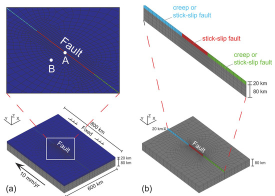
Figure 1.
(a) Finite-element mesh and velocity boundary condition of the fault model; (b) vertical strike-slip fault and its properties (modified from [34]).

Table 1.
Material parameters of the finite element model.
The velocity boundary conditions are shown in Figure 1. One boundary in the y direction was fixed, and the slip-rate of the other boundary was 10 cm/yr; the velocity did not change through the depths. It was assumed that there is no difference in the movement velocity of the upper crust, the middle and lower crust, and the upper mantle [35]; this assumption was also adopted in previous numerical simulation studies [36,37]. The bottom boundary of the model had a fixed normal displacement but free tangential displacement. The surface of the model was a free boundary.
We used a three-dimensional visco-elastic-plastic finite element parallel program for calculation. Studies using this program have been published in multiple papers, and the reliability of the program has been verified [29,30,33,38,39].
2.4. Analysis of the Synthesis Result
We ran the model a quasi-steady state after integrating for about 100,000 years (Figure 2a–c) until the regional stress patterns stabilized and the stress fluctuated around the background stress field as the result of earthquakes (modified from [34]). The predicted background stress was validated by its consistency with the regional stress field indicated by earthquake focal mechanisms [30]. In this state, the corresponding model stress field is called the background stress field, which reflects that the fault and the upper crust are in a critical plastic yielding state (Figure 2a–c). Then, fault failure led to stress reduction (Figure 2a,b), and the upper crust had a corresponding change in stress (Figure 2c). We observed that, after a modelled time of about 10,000 years, the stress on the fault plane (Figure 2a,b) and the upper crust (Figure 2c) had reached the steady state. This can be approximately regarded as the result of long-term tectonic movement or deformation of the crust. Our simulation of the steady-state background stress field is different from many previous numerical simulation studies, which did not simulate the steady-state background stress field but instead simply assumed a background stress field or an accumulated background stress field loaded by the boundary for a certain period [40,41]. We analyzed the simulation results after the model entered a steady-state loading state and generated a steady-state background stress field (see Figure 3 and Figure 4).
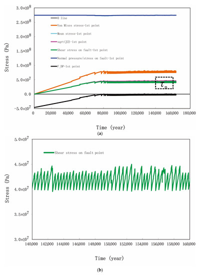
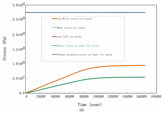
Figure 2.
Stress evolution. The model reached a steady-state deformation after 100,000 years (modified from [34]). (a) stress evolution at point A on the fault surface (point A has a depth of 10 km in the fault, see Figure 1); (b) The green curve is the shear stress on the vertical fault plane, zooming in of segment in black dash-line from (a). (c) stress evolution at point B on the fault surface (point B has a depth of 10 km in the upper crust outside the fault, see Figure 1). modified from [34].
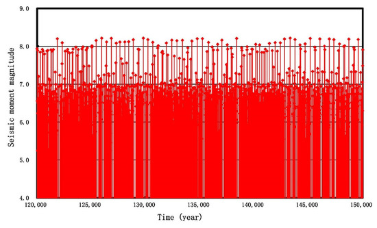
Figure 3.
The model calculated the earthquake activity on the fault. The horizontal axis is time, and the vertical axis is the magnitude of the earthquakes. We intercepted the data between 120,000–160,000 years when the model had entered a steady-state load time.
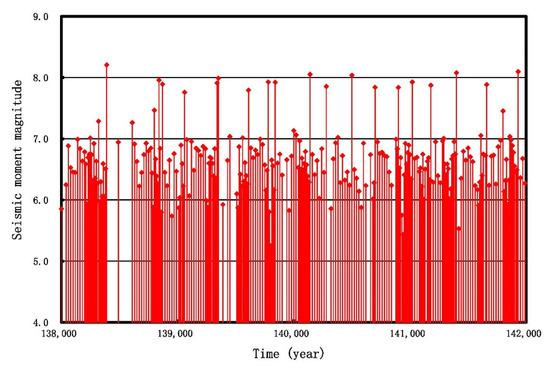
Figure 4.
Earthquake events between 130,000–140,000 years.
3. LSTM Modeling
LSTM is a time-recurrent neural network (RNN) [42,43]. Its emergence is to mitigate a weakness of RNN. The native RNN often encounters a vanishing gradient problem, that is, the nodes in the later time will have information attenuation, so that the long-term sequence cannot be transmitted, and the neural network is too deep to be trained. [44] conducted an in-depth study on this problem, and they found some fundamental reasons that make it difficult to train RNN. The LSTM network has memory because of the existence of connections between neural networks at different points in time, rather than the presence of feedforward or feedback in the network at a single point in time [45]. Therefore, we used LSTM modeling for the earthquake time series. Deep neural networks (DNNs) are highly suitable for processing big data. However, DNNs having many parameters are susceptible to overfitting problems, especially when the data is incomplete. Therefore, a drop-out technique can be adapted to provide an effective regularization method to avoid this problem [46,47]. The most important idea of the drop-out mechanism is that, in each training iteration, when the neural network updates a certain layer, it will randomly not update this layer or discard some neurons (based on the probability p). This means that part of the neural networks was sampled to be trained at this time in training iterations. In each training iteration, different parts of the network were sampled and trained. Based on the drop-out mechanism, neurons’ weights learned by back-propagation become a little insensitive to other neurons’ weights. Thus, the drop-out mechanism helps to prevent too much dependence on certain neurons of the network layer and reduces co-adaptability of neurons. During the test, all neurons of the network are kept (when drop-out is not used), but the activation rate is scaled by p (the drop-out probability). In view of the limited earthquake catalog, we wanted to discover the pattern of historical earthquakes and predict the event time and seismic moment magnitude of a certain earthquake inside the pre-earthquake data. The drop-out mechanism provided this possibility.
3.1. Data Preparation and Model Setting
The original data is a time series of earthquake events that enter the steady-state loading state obtained by geodynamic simulation. For ease of calculation, the event time and magnitude of earthquakes were normalized, and the pre-processed data was divided into a training dataset (67%) and a test dataset (33%).
In this work, we used historical earthquake data to predict the occurrence time and the magnitude of future earthquake events. For the current earthquake, events were quasi-periodic and related to the foreshock sequence. The time series forecast was classified as a regression problem. The input data was first put into the LSTM layer. The input-gate of the LSTM layer recombined the input data and decided which input data is important; this process is like principal component analysis (PCA). The LSTM layer can retain previous information, which helps improve the model’s ability to learn time series data. However, the structure of the model had some limitations. First, the initial parameters of the model affect the result. In addition, even though the LSTM layer has a strong ability to learn a time series, its fitting ability may be insufficient. Therefore, a fully-connected-layer was added on top of a single LSTM layer to promote learning ability. In addition, the drop-out was set on the LSTM layer to prevent overfitting.
3.2. Model Parameters
According to the magnitude of the earthquakes, the hidden layers disposed 100 neurons, and the output layer set 1 neuron (as a regression problem). The input variable was a time step (t−1) feature. The training used the adaptive momentum estimation algorithm (Adam) as the optimizer. The validation_data parameter was used in the fit function for recording the losses of the training dataset and the test dataset.
3.3. Model Validation
The mean-square error (MSE) was adopted as a loss function to evaluate the accuracy of the output results of the prediction model. RMSE is defined as Equation (13):
where N is the length of the input data; is the observation value in time i; and is the predicted value in time i.
The parameters and results of the evaluation are shown in Table 2.
Table 2.
LSTM model parameters.
Look_back is the time steps required to predict the next step; that is, LSTM considered that each input data is related to how many successively input data were previously input. Quasi-periodic earthquake events whose magnitudes were larger than an Mw of 6.5 could be learned in only 10 look_back windows in the earthquake time series. It is shown, in Figure 5a, that when window = 50 or 3, over-fitting and under-fitting occurred. The accuracy of prediction is shown in the MSE column (Table 1). Because of the different parameters used in the model training, the accuracy of different LSTM time series prediction models was different, but all met the requirements of earthquake magnitude prediction. After the output layer deformalized the results of the prediction output of the LSTM network and compared them to original data, we found that a look_back value of 10 was sufficient for good fit to the data and prediction (Figure 5b). Meanwhile, too many iterations led to over-fitting, and, therefore, poor prediction (epochs = 400).
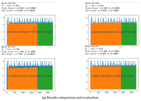
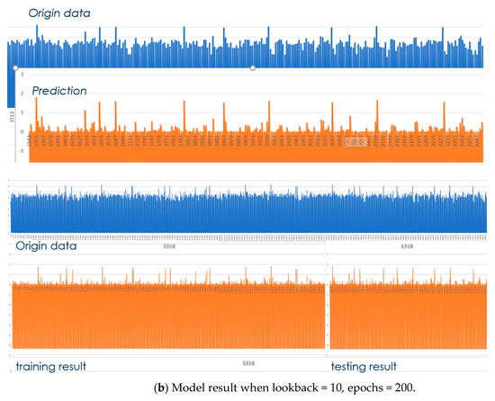
Figure 5.
Training and prediction results of the LSTM model.
We chose lookback = 10 and epochs = 200 as the final model parameters. The training and testing (prediction) results are shown in Figure 5b. It can be found from the comparison that the magnitude of earthquake events less than a Mw of 6.5 are not well fit and that the smaller magnitude the worse the fitting. However, magnitudes greater than an Mw of 6.5 could be successfully predicted. It was shown that smaller earthquakes, especially inter-seismic ones, occur more randomly (Figure 5b).
4. Discussion
We demonstrate from Figure 5 that the aftershock sequence pattern within a short period of time after the occurrence of a major earthquake can be well reproduced, and the shorter the period of the major earthquake, the better the prediction. However, the characteristics of a long inter-seismic sequence, especially when the stress release is large (a quiet period after a large earthquake), make it difficult to capture the seismic pattern. Regardless of the relative magnitude accuracy, the LSTM model is more sensitive and effective for time accuracy as a regression model, and the time parameter may correspond to the stress accumulation and release of a single strike-slip fault under the regional shear stress. We did not further tune and refine the LSTM model as this study case only considered one strike-slip fault and we did not add the rupture elements information in the geodynamic model to predict the location of the earthquakes. In this case, the LSTM model for earthquake prediction was a heuristic as a machine learning method test. In order to make the method more general for predicting the time, location, and magnitude of earthquakes, we must introduce a simulation based on the fault system model. In fact, there are many dependent factors for earthquake events. For example, they include the slip-rate of the fault, which is time-dependent and varies throughout the earthquake cycles. Other factors are: the fault geometry, the friction coefficient, regional loading conditions, etc.
5. Conclusions
With the help of machine learning we can use quantitative analysis of complete earthquake catalogs to reveal earthquake patterns and mechanical mechanisms. We have proposed here a LSTM model to solve this problem by synthesizing a complete earthquake catalog based on geodynamic simulation of a three-dimensional finite element fault model for more than 100,000 years. We also showed that the LSTM neural network model produced a meaningful result in time series prediction. Such a technique can be a method to quantify the earthquake cycle for prediction of earthquake events in the future.
As the model validation showed, the magnitude of earthquake events less than a Mw of 6.5 are not well-fit, and the smaller magnitude the worse fitting, indicating that smaller earthquakes, especially inter-seismic ones, occur more randomly. The application of the LSTM model showed a meaningful result of 0.08% in the MSE values. A successful prediction of the main shock being greater than an MW of 6.5 was obtained by the LSTM prediction model. Although, there were still errors in the prediction of the absolute magnitude value; the LSTM model was extremely sensitive to the time of earthquakes, which proves the prediction efficiency of the LSTM network.
However, while the time series of the single strike-slip fault earthquake catalog was tested for prediction, in the future, analysis of other factors, such as location, strain-stress, etc., of the earthquake catalog should be further applied to validate various machine learning methods to identify earthquake patterns. It is also necessary to test more variables on fault systems that are closer to real situations. Our research will continue to maximize the prediction performance of deep learning models by setting more complicated fault system models and optimizing models, while applying new algorithms and adding other variables that have causality with earthquake events. All these future efforts will require more high-performance computing, potentially over the cloud.
Author Contributions
Conceptualization, G.L., D.A.Y. and X.W. (Xianying Wang); methodology, C.C., X.W. (Xianying Wang), G.L. and D.A.Y.; software, G.L. and X.W. (Xianying Wang); validation, X.W. (Xianying Wang) and D.A.Y.; formal analysis, X.W. (Xianying Wang); investigation, C.C., L.Y. and Q.Z.; resources, X.W. (Xianying Wang), G.L. and X.W. (Xiangbin Wu); data curation, C.C., G.L. and X.W. (Xianying Wang); writing—original draft preparation, C.C. and X.W. (Xianying Wang); writing—review and editing, X.W. (Xianying Wang), C.C. and D.A.Y.; visualization, L.Y. and Q.Z.; supervision, X.W. (Xiangbin Wu) and G.L.; project administration, G.L.; funding acquisition, G.L. and D.A.Y. All authors have read and agreed to the published version of the manuscript.
Funding
This research was supported by the National Natural Science Foundation of China (41974107), the project of China Seismic Experimental Site (2019CSES0112), the National Key Research and Development Program of the Ministry of Science and Technology of China with the 2018YFC0603500 (2018–2020) and 2016YFC0600310 (2016–2020) projects, and U.S. Dept of Energy Grant DE-SC0019759 (D.A.Y.).
Institutional Review Board Statement
Not applicable.
Informed Consent Statement
Not applicable.
Data Availability Statement
Data available on request from the corresponding author.
Conflicts of Interest
The authors declare no conflict of interest.
References
- Cremen, G.; Galasso, C. Earthquake early warning: Recent advances and perspectives. Earth Sci. Rev. 2020, 205, 103184. [Google Scholar] [CrossRef]
- Mignan, A.; Ouillon, G.; Sornette, D.; Freund, F. Global Earthquake Forecasting System (GEFS): The Challenges Ahead. Eur. Phys. J. Spec. Top. 2021, 230, 473–490. [Google Scholar] [CrossRef]
- Geller, R.; Jackson, D.; Kagan, Y.; Mulargia, F. Earthquakes cannot be predicted. Science 1997, 275, 1616. [Google Scholar] [CrossRef]
- Peixoto, T.; Doblhoff-Dier, K.; Davidsen, J. Spatiotemporal correlations of aftershock sequences. J. Geophys. Res. 2010, 115. [Google Scholar] [CrossRef]
- Ogata, Y. Statistical models for earthquake occurrences and residual analysis for point processes. J. Am. Stat. Assoc. 1988, 83, 9–27. [Google Scholar] [CrossRef]
- Kagan, Y. Seismic moment distribution revisited: I. statistical results. Geophys. J. Int. 2002, 148, 520–541. [Google Scholar] [CrossRef]
- Kagan, Y.Y. Earthquakes: Models, Statistics, Testable Forecasts; American Geophysical Union: Washington, DC, USA, 2014. [Google Scholar]
- Mak, S.; Clements, R.; Schorlemmer, D. The statistical power of testing probabilistic seismic-hazard assessments. Seismol. Res. Lett. 2014, 85, 781–783. [Google Scholar] [CrossRef]
- Omori, F. On the aftershocks of earthquakes. J. Coll. Sci. Imp. Univ. Tokyo 1894, 7, 111–200. [Google Scholar]
- Utsu, T. Statistical study on the occurrence of aftershocks. Geophys. Mag. 1961, 30, 521–605. [Google Scholar]
- Utsu, T. Aftershocks and earthquake statistics (II): Further investigation of aftershocks and other earthquake sequences based on a new classification of earthquake sequences. J. Fac. Sci. Hokkaido Univ. Ser. Geophys. 1970, 3, 198–266. [Google Scholar]
- Ogata, Y. Estimation of the parameters in the modified omori formula for aftershock frequencies by the maximum likelihood procedure. J. Phys. Earth 1983, 31, 115–124. [Google Scholar] [CrossRef]
- Ogata, Y. Statistical model for standard seismicity and detection of anomalies by residual analysis. Tectonophysics 1989, 169, 159–174. [Google Scholar] [CrossRef]
- Ogata, Y. Space-time point-process models for earthquake occurrences. Ann. Inst. Stat. Math. 1998, 50, 379–402. [Google Scholar] [CrossRef]
- Mulargia, F.; Stark, P.; Geller, R. Why is probabilistic seismic hazard analysis (PSHA) still used? Phys. Earth Planet. Int. 2017, 264, 63–75. [Google Scholar] [CrossRef]
- Mega, M.; Allegrini, P.; Grigolini, P.; Latora, V.; Palatella, L.; Rapisarda, A.; Vinciguerra, S. Power-law time distribution of large earthquakes. Phys. Rev. Lett. 2003, 90, 188501. [Google Scholar] [CrossRef] [PubMed]
- Kagan, Y. Earthquake slip distribution: A statistical model. J. Geophys. Res. 2005, 110. [Google Scholar] [CrossRef]
- Greenhough, J.; Main, I. A poisson model for earthquake frequency uncertainties in seismic hazard analysis. Geophys. Res. Lett. 2008, 35. [Google Scholar] [CrossRef]
- Kagan, Y. Statistical distributions of earthquake numbers: Consequence of branching process. Geophys. J. Int. 2010, 180, 1313–1328. [Google Scholar] [CrossRef]
- Zhao, M.; Chen, S.; Yuen, A.D. Wenchuan earthquake aftershocks classification dataset. Digit. J. Glob. Chang. Data Repos. 2020. [Google Scholar] [CrossRef]
- Zhao, M.; Liao, S.; Huang, L. Development of auxiliary tools for automatic processing of seismic real-time stream data based on deep learning technology. Seismol. Geomagn. Obs. Res. 2020, 41, 165–171. [Google Scholar]
- Jordan, M.; Mitchell, T. Machine learning: Trends, perspectives, and prospects. Science 2015, 349, 255–260. [Google Scholar] [CrossRef]
- Schmidt, J.; Marques, M.; Botti, S.; Marques, M. Recent advances and applications of machine learning in solid-state materials science. NPJ Comput. Mater. 2019, 5, 83. [Google Scholar] [CrossRef]
- Bhusal, N.; Lohani, S.; You, C.; Hong, M.; Fabre, J.; Zhao, P.; Knutson, E.; Glasser, R.; Magaña-Loaiza, O. Front Cover: Spatial mode correction of single photons using machine learning. Adv. Quantum Technol. 2021, 4, 2170031. [Google Scholar] [CrossRef]
- Bergen, K.J.; Johnson, P.A.; Maarten, V.; Beroza, G.C. Machine learning for data-driven discovery in solid Earth geoscience. Science 2019, 363, eaau0323. [Google Scholar] [CrossRef]
- Mignan, A.; Broccardo, M. Neural network applications in earthquake prediction (1994–2019): Meta-analytic and statistical insights on their limitations. Seismol. Res. Lett. 2020, 91, 2330–2342. [Google Scholar] [CrossRef]
- Kim, Y.; Nakata, N. Geophysical inversion versus machine learning in inverse problems. Geophysics 2018, 37, 894–901. [Google Scholar] [CrossRef]
- Chen, M. Elastoplastic Mechanics; Science Press: Beijing, China, 2007. (In Chinese) [Google Scholar]
- Li, Q.; Liu, M.; Zhang, H. A 3-D viscoelastoplastic model for simulating long-term slip on non-planar faults. Geophys. J. Int. 2009, 176, 293–306. [Google Scholar] [CrossRef]
- Luo, G.; Liu, M. Stress evolution and fault interactions before and after the 2008 Great Wenchuan earthquake. Tectonophysics 2010, 491, 127–140. [Google Scholar] [CrossRef]
- Pande, G.; Beer, G.; Williams, J. Numerical methods in rock mechanics. Int. J. Rock Mech. Min. Sci. Geomech. Abstr. 1990, 27, 284. [Google Scholar]
- Kanamori, H.; Anderson, D.L. Theoretical basis of some empirical relations in seismology. Bull. Seismol. Soc. Am. 1975, 65, 1073–1095. [Google Scholar]
- Luo, G.; Liu, M. Multi-timescale mechanical coupling between the San Jacinto fault and the San Andreas fault, southern California. Lithosphere 2012, 4, 221–229. [Google Scholar] [CrossRef]
- Gao, Y.; Luo, G.; Sun, Y. Seismicity, fault slip rates, and fault interactions in a fault system. J. Geophys. Res. Solid Earth 2020, 125. [Google Scholar] [CrossRef]
- Wang, C.; Flesch, L.M.; Silver, P.G.; Chang, L.; Chan, W.W. Evidence for mechanically coupled lithosphere in central Asia and resulting implications. Geology 2008, 36, 363–366. [Google Scholar] [CrossRef]
- Xiao, J.; He, J. 3D finite-element modeling of earthquake interaction and stress accumulation on main active faults around the northeastern Tibetan Plateau edge in the past ∼100 years. Bull. Seismol. Soc. Am. 2015, 105, 2724–2735. [Google Scholar] [CrossRef]
- Zhu, S.; Zhang, P. FEM simulation of inter-seismic and co-seismic deformation associated with the 2008 Wenchuan Earthquake. Tectonophysics 2013, 584, 64–80. [Google Scholar] [CrossRef]
- Liu, M.; Luo, G.; Wang, H.; Stein, S. Long aftershock sequences in North China and Central US: Implications for hazard assessment in mid-continents. Earthq. Sci. 2014, 27, 27–35. [Google Scholar] [CrossRef]
- Wang, H.; Liu, J.; Shen, X.; Liu, M.; Li, Q.; Shi, Y.; Zhang, G. Influence of fault geometry and fault interaction on strain partitioning within western Sichuan and its adjacent region. Sci. China-Earth Sci. 2010, 53, 1056–1070. [Google Scholar] [CrossRef]
- Freed, A.M. Earthquake triggering by static, dynamic, and postseismic stress transfer. Annu. Rev. Earth Planet. Sci. 2005, 33, 335–367. [Google Scholar] [CrossRef]
- King, G.; Stein, R.S.; Lin, J. Static stress changes and the triggering of earthquakes. Bull. Seismol. Soc. Am. 1994, 84, 935–953. [Google Scholar]
- Hochreiter, S.; Schmidhuber, J. Long short-term memory. Neural Comput. 1997, 9, 1735–1780. [Google Scholar] [CrossRef] [PubMed]
- Olah, C. Understanding LSTM Networks—Colah’s Blog. Available online: https://colah.github.io/posts/2015-08-Understanding-LSTMs/ (accessed on 19 April 2021).
- Bengio, Y.; Simard, P.Y.; Frasconi, P. Learning long-term dependencies with gradient descent is difficult. IEEE Trans. Neural Netw. 1994, 5, 157–166. [Google Scholar] [CrossRef] [PubMed]
- Graves, A.; Schmidhuber, J. Framewise phoneme classification with bidirectional LSTM and other neural network architectures. Neural Netw. 2005, 18, 602–610. [Google Scholar] [CrossRef] [PubMed]
- Hinton, G.E.; Srivastava, N.; Krizhevsky, A.; Sutskever, I.; Salakhutdinov, R. Improving neural networks by preventing co-adaptation of feature detectors. arXiv 2012, arXiv:1207.0580. [Google Scholar]
- Srivastava, N.; Hinton, G.E.; Krizhevsky, A.; Sutskever, I.; Salakhutdinov, R. Dropout: A simple way to prevent neural networks from overfitting. J. Mach. Learn. Res. 2014, 15, 1929–1958. [Google Scholar]


Publisher’s Note: MDPI stays neutral with regard to jurisdictional claims in published maps and institutional affiliations. |
© 2021 by the authors. Licensee MDPI, Basel, Switzerland. This article is an open access article distributed under the terms and conditions of the Creative Commons Attribution (CC BY) license (https://creativecommons.org/licenses/by/4.0/).