A Systematic Framework for State of Charge, State of Health and State of Power Co-Estimation of Lithium-Ion Battery in Electric Vehicles

Abstract

Due to its advantages of high voltage level, high specific energy, low self-discharging rate and relatively longer cycling life, the lithium-ion battery has been widely used in electric vehicles. To ensure safety and reduce degradation during the lithium-ion battery’s service life, precise estimation of its states like state of charge (SOC), capacity and peak power is indispensable. This paper proposes a systematic co-estimation framework for the lithium-ion battery in electric vehicle applications. First, a linearized equivalent circuit-based battery model, together with an affine projection algorithm is used to estimate the model parameters. Then the state of health (SOH) estimator is triggered weekly or semi-monthly offline to update capacity based on the three-dimensional response surface open circuit voltage model and particle swarm optimization algorithm for accurate online SOC and state of power (SOP) estimation. At last, the Unscented Kalman Filter utilizes the estimated model parameters and updated capacity to estimate SOC online and the SOP estimator provides the power limitations considering SOC, current and voltage constraints, taking advantage of the information from both SOH and SOC estimators. Experiments show that the relative error of the SOH estimator is under 1% in all aging states whatever the loading profile is. The mean absolute SOC estimation error is under 1.6% even when the battery undergoes 744 aging cycles. The SOP estimator is validated by means of the calibrated battery model based on the HPPC test and its performance is ideal.

1. Introduction

Under the trend of the electrification of the global automotive industry, power batteries used for electric vehicles (EVs) should have high specific energy, high specific power, better safety performance, longer cycle life and lower cost [1,2]. Lithium-ion batteries, especially lithium nickel-manganese-cobalt oxide (LiNMC) and lithium iron phosphate (LiFePO4) batteries, have dominated the automotive industry due to their satisfaction of the above strict requirements [3,4]. In 2020, over 39.7 GWh LiNMC power batteries were installed in EVs in China [5].

The EV industry is one of the mainstay industries of China’s economy. However, in 2020, the outbreak of COVID-19 had a great negative impact on both the manufacturing and sales of EVs. To further guide and support the healthy development of the EV industry, on 24 July 2020, the Ministry of Industry and Information Technology of the People’s Republic of China issued the “Regulations of the Ministry of Industry and Information Technology of the People’s Republic of China on modifying the management of new energy vehicle production enterprises and product admittance”, which relaxed the admittance of EVs, aiming at promoting the technological upgrading of the EV industry. Besides its economic benefits, the development of EVs is also beneficial for reducing CO₂ emissions and improving economic efficiency [6,7]. However, EV technology still confronts bottlenecks such as accurate state estimation for the power battery. During the actual operation of EVs, the external load and use environment of the power battery are very complex. Both its charging and discharging procedures are nonlinear and complex processes including a variety of energy conversion reactions [8,9]. In addition, the performance of the power battery is significantly distinct in different working conditions and aging states. Therefore, the estimation of battery states, including state of charge (SOC), state of health (SOH) and state of power (SOP), will deviate from the real value greatly if the traditional estimation method is used. Obtaining these hidden states with high precision has posed a great challenge for current battery management system (BMS) technology [10,11].

1.1. Review of Existing Battery State Estimation Methods

The SOC represents the remaining charge of the battery. Traditional SOC estimation methods include the ampere-hour counting approach, model-based open-circuit voltage (OCV) method, resistance-based estimation method, etc. [12]. However, these methods cannot guarantee precision if sensors are suffering from severe measurement noise or the vehicle operates in an extremely dynamic environment. Thus, approaches based on filtering methods were widely researched in recent years given their accuracy and robustness [13]. For example, W He et al. [14] present an electrochemical model involving the battery’s internal physical and chemical properties for lithium-ion battery SOC estimation using a novel projection-based filtering method. Considering that the performance of the Kalman filter is largely dependent on the accuracy of the adopted battery model, updating the model parameters is necessary to ensure precise SOC estimation throughout the battery’s entire life and under various working conditions.

The SOH characterizes the ability of the current battery to store electric energy relative to a new battery. Currently, the most widely used index for SOH is the ratio of current capacity to initial capacity. Existing methods for SOH estimation include differential voltage analysis (DVA), incremental capacity analysis (ICA) and the empirical model-based method, etc. However, the ICA/DVA method is only applicable under constant-current charge or discharge circumstances [15]. Empirical model construction requires time-consuming and laborious accelerating aging experiments under various environmental conditions. Thus, both ICA/DVA and empirical model-based methods are difficult to apply directly for SOH estimation on EVs. A simple yet effective approach to estimate SOH is through the OCV-SOC look-up table [16]. The SOC variation during a certain period can be determined by looking up the OCV corresponding to the start and end points of the time period. Then dividing the ampere-hour value by SOC variation, the capacity and SOH estimation results can be obtained.

The SOP is the parameter used to describe the maximum charging and discharging capabilities of the battery, which is usually constrained by multiple thresholds such as voltage limits, current limits and SOC limits [17]. The equivalent circuit model (ECM)-based approach is currently the most widely applied method in SOP estimation, as in Refs. [18,19]. To ensure the estimation accuracy in a wide range of different working conditions, the adaption of model parameters is required as SOP is heavily related to them.

So far, most research focuses on just one state estimation of the battery because as the number of estimation states increases, the complexity of the estimation algorithm will increase as well. However, given the fact that these three state parameters are strongly correlated with each other, it is more suitable to incorporate them under a systematic co-estimation framework to realize higher fidelity estimation results. A few studies have worked on the combined estimation of two states. For example, Y Zou et al. [20] included capacity into the state equation of the battery model and realized combined SOC-SOH estimation. Dong et al. [21] proposed the Kalman Filter-based SOC-SOP co-estimated method. L Zheng et al. [22] proposed trial proportional-integral (PI) observers with a reduced physics-based electrochemical model to simultaneously estimate SOC and SOH for lithium-ion batteries. Similar work is also down in Ref. [23] but just as Ref. [24] pointed out, even two states can hardly guarantee the accurate estimation of the real status of the battery due to the close relationship among the three states. In addition, the co-estimation mechanism could facilitate sharing of the adaptive estimation results of the model parameters. Thus, Ref. [24] put forward a co-estimation scheme of SOC, SOH and SOP for lithium-ion battery and embedded the algorithm in a real BMS controller and the outcome performance was desirable. However, there are still some drawbacks to the approach in Ref. [24]. First, the authors did not consider the changing of the OCV-SOC curve as the battery ages. Second, when estimating OCV and resistance of the battery, the authors used the linear Rint model, which cannot capture the characteristics of the battery under dynamic current loads, thus may degrade the estimation accuracy of relevant parameters and states. Third, the impact of SOC constraints on SOP is not included, making the SOP estimation algorithm less comprehensive.

1.2. Contribution of This Study

The main focus of this study is to establish a systematic framework for SOC, SOH and SOP co-estimation of lithium-ion batteries in electric vehicles, which is accurate and robust under different loading profiles and different levels of degradation. The most outstanding feature that distinguishes our research from the existing literature is that we systematically cope with the intertwin relationship between SOC, SOH and SOP. Most existing research only focuses on the estimation of one state, seldom does the literature focus on the co-estimation of two states. In detail, three contributions have been made with the proposed co-estimation method:

(1) 

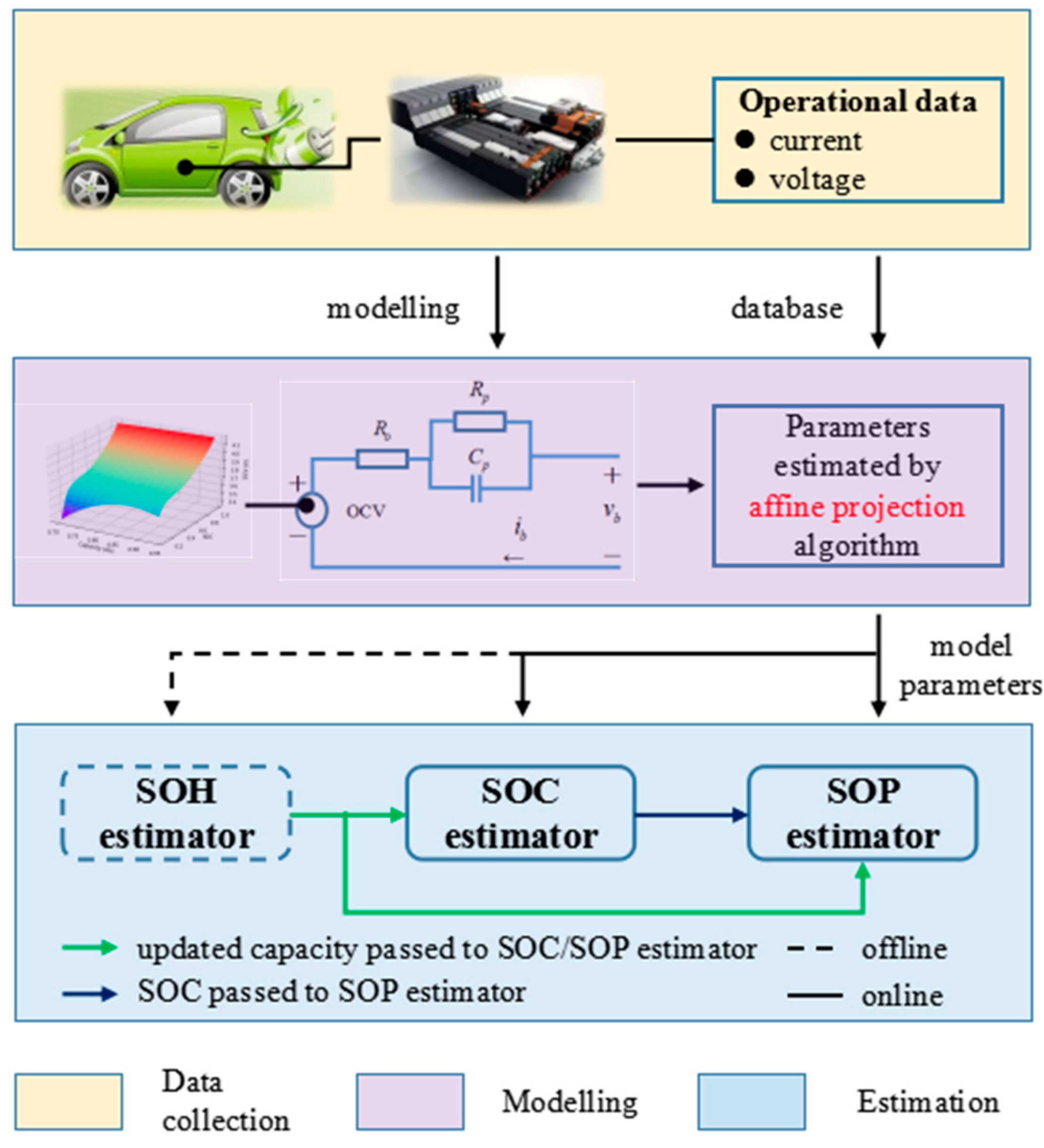
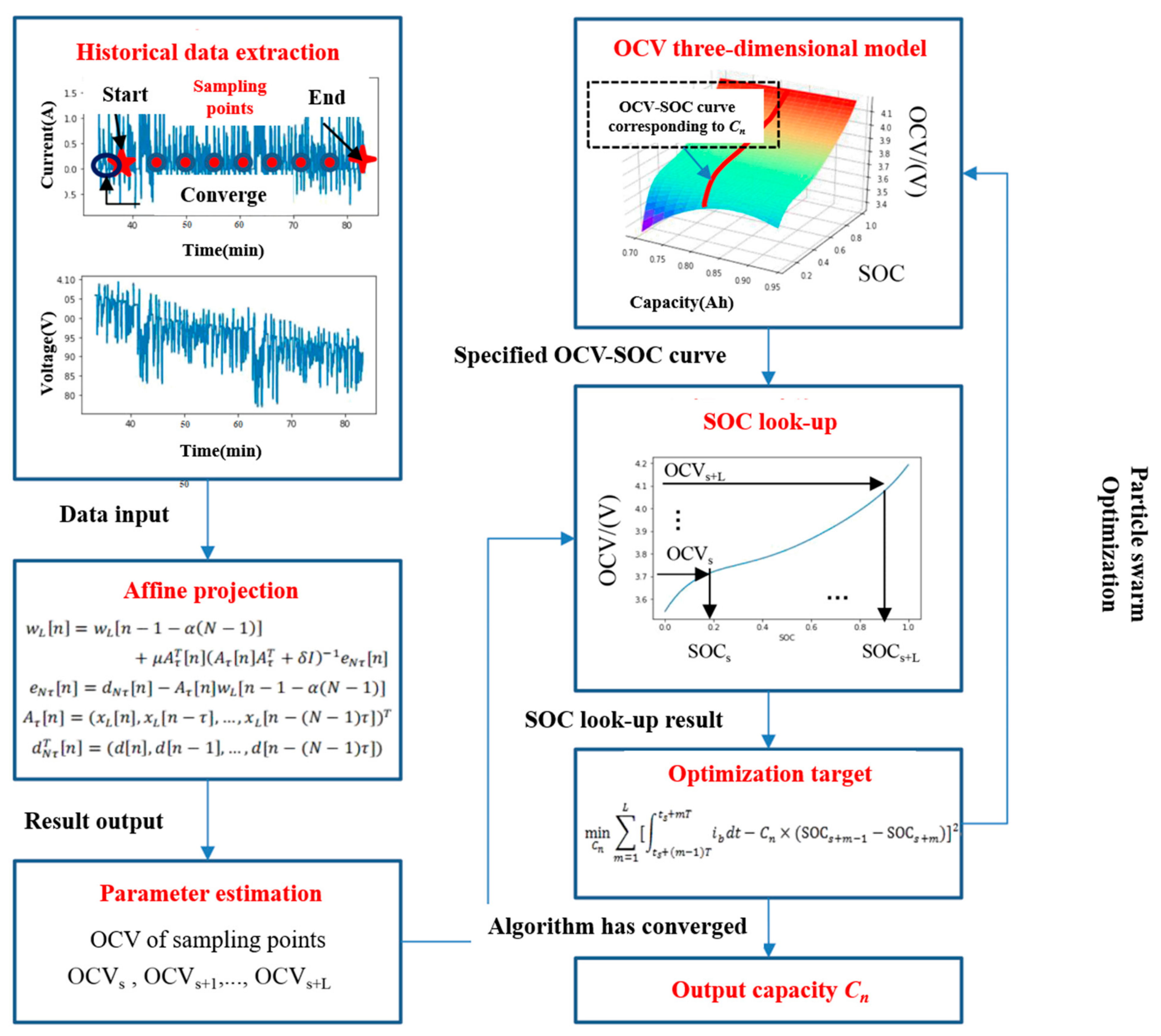
Parameter estimation: A linearized first-order RC ECM is adopted to reflect the dynamic properties of the battery and an affine projection (AP) algorithm is used to estimate the model parameters online for the first time. The ideal performance of the AP algorithm lies in the fact that it is effective especially when input data are highly correlated [25], which is just the case for the RC ECM due to the “memory property” introduced by the RC network. The adaptive estimation method makes it unnecessary to calibrate the model parameters through laborious experiments, which is error-prone and time-consuming.

(2) 

SOH estimator: To describe the varying characteristics between OCV and SOC at distinct degradation states, the three-dimensional response surface-based OCV-SOC model [26] is used in this paper, which is proposed by X Rui et al. [27] and verified to be effective and accurate in SOC and SOH estimation. The model is then combined with a particle swarm optimization (PSO) algorithm to constitute the novel SOH estimator. Because of the strong optimality performance of the PSO algorithm, the estimated SOH could be very close to the true value. Results show that the SOH estimation error is under 0.51% under various working conditions.

(3) 

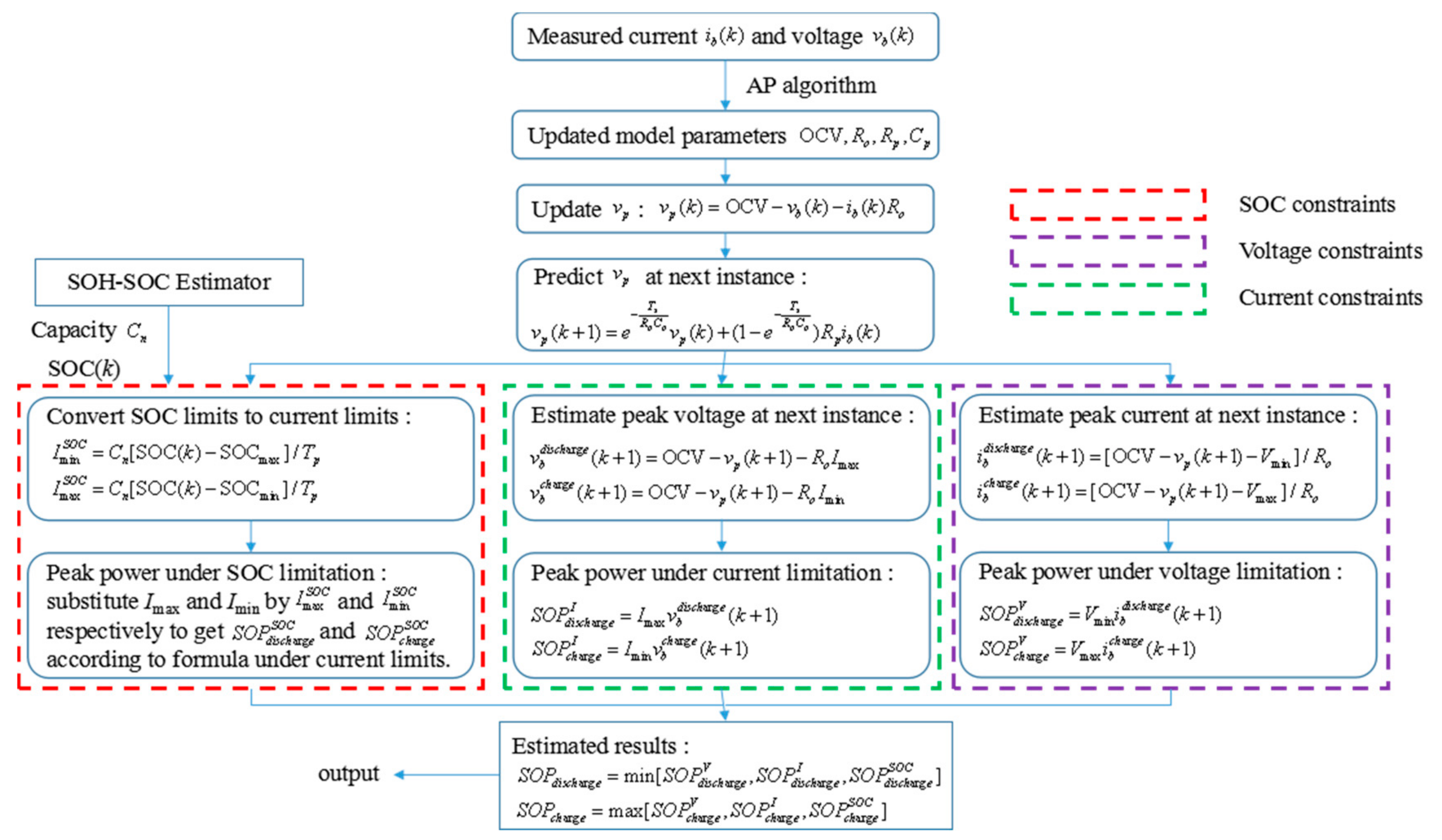
SOP estimator: Current, voltage and SOC constraints are included in the SOP estimation algorithm and the interaction effect between these constraints is discussed in discharging conditions, which is rare in the existing literature.

1.3. Organization of This Paper

The remainder of this paper is organized as follows. Section 2 introduces the general framework of the proposed co-estimation algorithm and detailed descriptions of the SOC, SOH and SOP estimators respectively. Section 3 describes the battery experiment briefly. Section 4 validates the proposed co-estimation algorithm under various working conditions and different levels of aging states. Section 5 concludes the whole paper.

2. The Proposed Co-Estimation Algorithm

Figure 1 plots the scheme of the co-estimation algorithm. The main steps of the estimation method are summarized as follows. Firstly, when the battery capacity needs to be updated, the estimator estimates the OCV based on the AP algorithm and then looks up the corresponding SOC variation based on the three-dimensional response surface OCV model to give the SOH estimation result. It needs to be highlighted here that it needs to look up SOC according to the OCV estimation and the three-dimensional response surface model, during which the intertwined relationship between SOC and SOH is considered to some extent. Then, during vehicle operation, the SOC estimator utilizes the battery capacity from the SOH estimator and online updated battery model parameters given by the AP algorithm to estimate SOC based on the Unscented Kalman Filter (UKF) algorithm. At last, the maximum charge and discharge power under the constraints imposed by current, voltage and SOC limitations are predicted by the SOP estimator according to the estimation results from both the SOH and SOC estimators. The detailed descriptions of the three estimators are expanded in the following subsections.

2.1. Battery Modeling and Online Parameter Estimation

The first-order RC ECM, as shown in Figure 2, is widely used in battery state estimation as it can relatively precisely reflect the nonlinear input-output relationship of the battery while keeping the computational complexity within a certain level. The main components of the first-order RC ECM include a voltage source, an ohmic resistance R_o and an RC network, which comprises polarization resistance R_p and polarization capacitance C_p. The method to identify the model parameters using HPPC response is also denoted in Figure 2. Here, the OCV is a function of both SOC and capacity, which can be expressed by the three-dimensional response surface model as Equation (1):

$$\mathrm{OCV}(\mathrm{SOC},C_n)={\displaystyle \sum _{i=0}^{np}{c}_i\times {(\mathrm{SOC})}^i}$$

(1)

where n_p represents the polynomial order of OCV with respect to SOC [28,29]. c_i represents the polynomial coefficient and it is the two-order polynomial function of capacity C_n. Figure 3 shows the detailed value of parameters c_i based on the HPPC test. The polynomial coefficients in Figure 3 are calibrated based on HPPC tests under different aging states. At a specific degradation level, the OCV-SOC coefficients can be determined using the method introduced in Section 4.1 below, then combing all the OCV-SOC coefficients in different aging levels with calibrated capacity, the polynomial coefficients in Figure 3 can be derived.

The dynamic characteristics of first-order RC ECM can be expressed by the following Equations (2) and (3):

$$C_p{\dot{v}}_p+\frac{v_p}{R_p}=i_b$$

(2)

$$v_b=\mathrm{OCV}-v_p-i_b{R}_0$$

(3)

where v_p is the voltage across the RC network, i_b represents the outflow current (positive for discharging and negative for charging) and v_b represents the terminal voltage.

Through z-transformation, the autoregressive exogenous (ARX) model of the battery can be derived based on Equations (2) and (3), which can be expressed as following Equations (4)–(6) [30]:

$$y_k={\theta }_k^T{x}_k$$

(4)

$$x_k={[-i_b(k),-i_b(k-1),\mathrm{OCV}(k-1)-v_b(k-1),1]}^T$$

(5)

$${\theta }_k={[{\theta }_1,{\theta }_2,{\theta }_3,{\theta }_4]}^T={[R_o,-R_o+\frac{T_s}{C_t}+\frac{T_s{R}_o}{C_t{R}_t},\frac{T_s}{C_t{R}_t}-1,\mathrm{OCV}]}^T$$

(6)

where k represents the step index. T_s denotes the data sampling period.

In this paper, the AP algorithm is used to estimate the ARX parameters adaptively. Because the AP algorithm has desirable estimation performance over correlated input data, it is suitable for the first-order RC ECM battery model as the RC network introduces the “memory property”.

Let w_L[n] represent the L adaptive filter coefficients and w_L[n]x_L[n] = d[n] denotes the linear model, then the updated equation can be expressed as Equations (7)–(10):

$$w_L[n]=w_L[n-1-\alpha (N-1)]+\mu A_{\tau }^T[n]{(A_{\tau }[n]A_{\tau }^T[n]+\delta I)}^{-1}{e}_{N\tau }[n]$$

(7)

$$e_{N\tau }[n]=d_{N\tau }[n]-A_{\tau }[n]w_L[n-1-\alpha (N-1)]$$

(8)

$$A_{\tau }[n]=(x_L[n],x_L[n-\tau ],\dots ,x_L[n-(N-1)\tau ]{)}^T$$

(9)

$$d_{N\tau }^T[n]=(d[n],d[n-\tau ],\dots ,d[n-(N-1)\tau ])$$

(10)

where N is the length of the input signal. μ is the update step size. δ represents the initial offset covariance. α and τ control the interval between the update term and its base term for the coefficients and input signals, respectively. Here, the most frequently used standard AP algorithm where δ = 0, α = 0 and τ = 1 is adopted.

After estimating the parameter matrix θ_k using the AP algorithm, the battery model parameters can be obtained through the following Equations (11)–(14):

$$\mathrm{OCV}={\theta }_4$$

(11)

$$R_o={\theta }_1$$

(12)

$$R_t=\frac{{\theta }_2-{\theta }_1{\theta }_3}{1+{\theta }_3}$$

(13)

$$C_t=\frac{T_s}{{\theta }_2-{\theta }_1{\theta }_3}$$

(14)

2.2. PSO Based SOH Estimator

In this paper, the particle swarm optimization (PSO) algorithm is adopted to construct the SOH estimator. PSO is a kind of evolutionary computing technology, which was proposed by Dr. Eberhart and Dr. Kennedy in 1995 [31]. It originated from research on the behavior of bird’s predation. The algorithm is initially inspired by the regularity of bird cluster activities. Based on the observation of the behavior of animal groups, PSO makes use of the information sharing of individuals in the group to make the movement of the whole group evolve from disorder to order in the problem-solving space, so as to obtain the optimal solution.

PSO is initialized as a group of random particles. In each iteration, the particles update themselves by tracking two “extremum”: the first is the best solution found by the particles themselves, which is called the individual extremum point and represented by pbest. Its iteration rule is as Equation (15):

$${\mathrm{pbest}}_i(t+1)=\left\{\begin{array}{c}{\mathrm{pbest}}_i(t)\hspace{1em}\mathrm{if} f(Xi(t+1))\ge f({\mathrm{pbest}}_i(t))\\ X_i(t+1)\hspace{1em}\mathrm{if} f(X_i(t+1))<f({\mathrm{pbest}}_i(t))\end{array}\right.$$

(15)

where X_i = [x_i1,x_i2,...,x_in] is the current location of particle i. The other extremum point is the best solution found by the whole population, which is called the global extremum and labeled as gbest, which means as Equation (16):

$${\mathrm{gbest}}_i(t)=\min \left\{f({\mathrm{pbest}}_1(t)),f({\mathrm{pbest}}_2(t)),\dots ,f({\mathrm{pbest}}_N(t))\right\}$$

(16)

After finding the two “extremum”, the particle updates its velocity and position according to the following Equations (17)–(18):

$$v_{ij}(t+1)=m{v}_{ij}(t)+c_1{r}_1({\mathrm{pbest}}_{ij}(t)-x_{ij}(t))+c_2{r}_2({\mathrm{gbest}}_{ij}(t)-x_{ij}(t))$$

(17)

$$x_{ij}(t+1)=x_{ij}(t)+v_{ij}(t+1)$$

(18)

where m is the inertia coefficient. c₁ and c₂ are the cognitive and social parameters respectively. r₁, r₂ are both random numbers in range [0, 1].

Figure 4 demonstrates the framework of the proposed SOH estimator. The estimation process can be expressed as follows: First, historical data of the last driving event, including battery current and voltage, are extracted. Then, several sampling points, which are evenly distributed between the start and end points, are selected for OCV estimation using the AP algorithm. It needs to be noticed that the start point here does not mean the first point of the historical data. Because the initial OCV guess may deviate from the true value largely, a relatively reasonable length of data after the first point is left out for OCV estimation convergence. At last, the following target function is minimized by combining the three-dimensional response surface OCV model and PSO algorithm to give the capacity estimation as Equation (19) [32]:

$$\underset{C_n}{\min }{\{{\displaystyle \sum _{m=1}^L[{\displaystyle \underset{t_s+(m-1)T}{\overset{t_s+mT}{\int }}{i}_b\mathrm{d}t}-C_n\times ({\mathrm{SOC}}_{s+m-1}-{\mathrm{SOC}}_{s+m})]}\}}^2$$

(19)

where L is the number of the sampling points. T represents the time interval between adjacent sampling points. The concept behind the method is to find the OCV-SOC curve that best fits the equation relationship between (SOC_{s + m − 1}-SOC_{s + m}) × C_n and ${\displaystyle \underset{t_s+(m-1)T}{\overset{t_s+mT}{\int }}{i}_b\mathrm{d}t}$ because both of them refer to the amount of electricity consumed over the trip. The intertwin relationship between SOC and SOH is incorporated in the three-dimensional response surface model. The capacity corresponding to the best suitable OCV-SOC curve is the estimation result.

It needs to be highlighted here that the SOH estimator does not need to be operated online. The SOH estimation can be conducted when the vehicle is parked because the parking state ensures that BMS is relatively free, so the computational burden does not hinder the normal operation of the vehicle. In addition, the slow-varying property of the capacity also guarantees the offline estimation to be applicable and accurate. Due to the above assumption, the following SOC estimation and current SOH estimation results do not come from the same timestamp. However, it does not violate the “co-estimation” idea because the error introduced can be kept within a certain level.

2.3. UKF-Based SOC Estimator

Considering the nonlinear property of the first-order ECM battery model, the UKF is applied to estimate SOC. Unlike the Extended Kalman Filter (EKF), which attempts to linearize the nonlinear functions and is also widely used in SOC estimation, the UKF selects a handful of “sigma points”, passes them through the appropriate function, then finally re-estimates a normal distribution around those propagated points. Case studies have shown that UKF is superior to EKF in nearly all scenarios. The main steps of UKF are summarized in

Table 1. Summary of the Unscented Kalman Filter algorithm.

$\mathbf{State} \mathbf{equation}: {\mathit{x}}_{\mathit{k}+1}={\mathit{f}}_{\mathit{k}}({\mathit{x}}_{\mathit{k}},{\mathit{u}}_{\mathit{k}},{\mathit{v}}_{\mathit{k}})$ $\mathbf{Measurement} \mathbf{equation}: {\mathit{z}}_{\mathit{k}}={\mathit{h}}_{\mathit{k}}({\mathit{x}}_{\mathit{k}},{\mathit{u}}_{\mathit{k}},{\mathit{w}}_{\mathit{k}})$

Step 1: Choose n+1 sigma points $x^{(0)}=\overline{x}=E(x)$, $x^{(i)}=x^{(0)}+{(\sqrt{(n+\kappa )P})}_i^T$, $x^{(n+i)}=x^{(0)}-{(\sqrt{(n+\kappa )P})}_i^T$, i=1,2,…,n where ${(\sqrt{(n+\kappa )P})}_i$ is the ith row of the matrix square root $(\sqrt{(n+\kappa )P})$. Weights of the sigma points are $W^{(0)}=\frac{\kappa }{n+\kappa },$ $W^{(i)}=\frac{1}{2(n+\kappa )},$ i = 1,2,…,2n Step 2: State prediction (a priori) $x^{(i)}(k+1\left|k\right.)=f_k(x^{(i)}(k\left|k\right.),u_k,v_k)$ $\widehat{x}(k+1\left|k\right.)={\displaystyle \sum _{i=0}^{2n}{W}^{(i)}{x}^{(i)}(k+1\left|k\right.)}$ Step 3: Calculate estimate covariance prediction (a priori) $P(k+1\left|k\right.)=Q_k+{\displaystyle \sum _{i=0}^{2n}{W}^{(i)}[x^i(k+1\left|k\right.)-\widehat{x}}(k+1\left|k\right.)]{[x^{(i)}(k+1\left|k\right.)-\widehat{x}(k+1\left|k\right.)]}^T$ Step 4: Calculate innovation $z^{(i)}(k+1\left|k\right.)=h(x^{(i)}(k+1\left|k\right.),u_k,w_k)$ $\widehat{z}(k+1\left|k\right.)={\displaystyle \sum _{i=0}^{2n}{W}^{(i)}{z}^{(i)}(k+1\left|k\right.)}$ Step 5: Calculate Kalman gain $P_{yy}(k+1\left|k\right.)=P_k+{\displaystyle \sum _{i=0}^{2n}{W}^{(i)}[z^{(i)}(k+1\left|k\right.)-\widehat{z}}(k+1\left|k\right.)]{[z^{(i)}(k+1\left|k\right.)-\widehat{z}(k+1\left|k\right.)]}^T{P}_{xy}(k+1\left|k\right.)$ $P_{xy}(k+1\left|k\right.)={\displaystyle \sum _{i=0}^{2n}{W}^{(i)}[x^{(i)}(k+1\left|k\right.)-\widehat{x}}(k+1\left|k\right.)]{[z^{(i)}(k+1\left|k\right.)-\widehat{z}(k+1\left|k\right.)]}^T$ $K_k=P_{xy}(k+1\left|k\right.)P_{yy}{(k+1\left|k\right.)}^{-1}$ Step 6: State estimate update (a posterior) $\widehat{x}(k+1\left|k\right.+1)=\widehat{x}(k+1\left|k\right.)+K_k(z_k-\widehat{z}(k+1\left|k\right.))$ Step 7: Calculate estimate covariance update (a posterior) $P(k+1\left|k\right.+1)=P(k+1\left|k\right.)+K_k{P}_{yy}(k+1\left|k\right.)K_k^T$

[33].

The discrete-time format of the battery model based on Equations (2) and (3) can be written as Equations (20) and (21) [34]:

$$x_{k+1}=\left[\begin{array}{cc}1& 0\\ 0& e^{-\frac{T_s}{R_p{C}_p}}\end{array}\right]x_k+\left[\begin{array}{c}\frac{-\eta T_s}{3600C_n}\\ R_o(1-e^{-\frac{T_s}{R_p{C}_p}})\end{array}\right]u_k+v_k$$

(20)

$$y_k=\mathrm{OCV}(\mathrm{SOC},C_n)-[0\hspace{0.33em}\hspace{0.33em}1]x_k-R_o{u}_k+w_k$$

(21)

where state vector x = [SOC,v_p]^T, input u_k refers to the excitation current i_b while output y_k is the terminal voltage v_b. v_k and w_k represent the process and measurement noise, respectively. η is the coulomb efficiency.

The SOC estimation procedure is as follows. From the SOH estimator, the battery capacity is updated first and stays constant during SOC estimation considering its slow variation property. Then, during vehicle operation, the model parameters are estimated online based on the AP algorithm and updated with period T_s. According to the discrete-time battery model and UKF algorithm, the SOC is estimated and updated simultaneously.

2.4. Multi-Constraint SOP Estimator

For safe and durable operation, the working current, voltage and SOC of lithium-ion batteries must be restricted within a suitable range [35] and battery power (positive for discharge and negative for charge) will be limited by these restrictions. The flowchart of the proposed SOP estimation algorithm is shown in Figure 5. It needs to be noticed that the SOH-SOC estimator provides reliable battery capacity and SOC values to the SOP estimator so that the SOP limits under the SOC constraint can be achieved with high confidence. Detailed descriptions are as follows [36].

First, consider the power limits under voltage constraints. The voltage across the RC network at the current time step k can be calculated according to the Equation (22):

$$v_p(k)=\mathrm{OCV}-v_b(k)-i_b(k)R_o$$

(22)

Then, its prediction value at the next time step can be derived based on the discretized form of Equation (2), as Equation (23):

$$v_p(k+1)=e^{-\frac{T_s}{R_p{C}_p}}{v}_p(k)+(1-e^{-\frac{T_s}{R_p{C}_p}})R_p{i}_b(k)$$

(23)

Then, the current limits corresponding to the upper and lower voltage limits are calculated as Equation (24):

$$i_b^{discharge}(k+1)=\left[\mathrm{OCV}-v_p(k+1)-V_{\min }\right]/R_p$$

(24)

where V_max and V_min represent the upper and lower cut-off voltage respectively.

At last, the power limits at charge and discharge conditions constrained by voltage limits as Equations (25) and (26):

$$SO{P}_{discharge}^V=V_{\min }{i}_b^{discharge}(k+1)$$

(25)

$$SO{P}_{charge}^V=V_{\max }{i}_b^{charge}(k+1)$$

(26)

Then consider the power limits under current constraints. Same as described above, the voltage across the RC network at the next time step needs to be first calculated according to Equations (22) and (23). Then, the voltage limits corresponding to the upper and lower current limits are calculated by Equations (27) and (28):

$$v_b^{discharge}(k+1)=\mathrm{OCV}-v_p(k+1)-R_o{I}_{\max }$$

(27)

$$v_b^{charge}(k+1)=\mathrm{OCV}-v_p(k+1)-R_o{I}_{\min }$$

(28)

where I_max and I_min represent the maximum and minimum current, respectively. At last, the power limits at charge and discharge conditions constrained by current limits as Equations (29) and (30):

$$SO{P}_{discharge}^I=I_{\max }{v}_b^{discharge}(k+1)$$

(29)

$$SO{P}_{charge}^I=I_{\min }{v}_b^{charge}(k+1)$$

(30)

Finally, consider the power limits under SOC constraints. The polarization voltage over the RC network still has to be derived from Equations (22) and (23) first. The current limits under SOC constraints can be calculated by Equations (31) and (32):

$$I_{\min }^{SOC}=C_n\left[SOC(k)-SO{C}_{\min }\right]/T_p$$

(31)

$$I_{\max }^{SOC}=C_n\left[SOC(k)-SO{C}_{\max }\right]/T_p$$

(32)

where SOC_max and SOC_min represent the designed upper and lower cut-off SOC respectively, T_p denotes the time window size, which can be tuned to determine when the SOC constraint is triggered. For the discharging process, a longer T_p means lower current constraints, thus an earlier trigger of SOC constraints. Because Equation (31) and Equation (32) have converted the SOC limitations to current limitations, the peak power under SOC limitation for discharging and charging process (denoted as ${SOP}_{discharge}^{\mathrm{SOC}}$ and ${SOP}_{charge}^{\mathrm{SOC}}$ respectively) can be derived from the same formula under the current constraint.

Ultimately, the battery power will be limited by the minimum absolute value of the above-mentioned three constraints, which means as Equation (33):

$$\left\{\begin{array}{l}SO{P}_{discharge}=\min \left[SO{P}_{discharge}^V,SO{P}_{discharge}^I,SO{P}_{discharge}^{\mathrm{SOC}}\right]\hfill \\ SO{P}_{charge}=\max \left[SO{P}_{charge}^V,SO{P}_{charge}^I,SO{P}_{charge}^{\mathrm{SOC}}\right]\hfill \end{array}\right.$$

(33)

3. Design of Battery Experiment

Eight battery cells are experimented on, on the platform constituting a thermal chamber, an Arbin BT2000 tester, a computer for data recording and a switchboard for cable connection. The test mainly includes constant charge and constant discharge aging cycles. When the battery undergoes a certain number of cycles, characteristic tests including the hybrid pulse power characteristic (HPPC) test, dynamic stress test (DST), federal urban dynamic schedule (FUDS) and capacity calibration test are conducted to check the battery dynamic property. During these tests, battery current and voltage are recorded with a frequency of 10 Hz. For detailed information on the battery experiment, please refer to Ref. [37]. In this paper, only data under normal room temperature, namely 22 °C, are used.

4. Verification and Discussion

In this section, the effectiveness of the proposed method is validated under different working conditions (including HPPC, DST and FUDS tests) and different levels of aging states. The performance of the model parameter estimation method, together with SOH/SOC/SOP estimators, is evaluated.

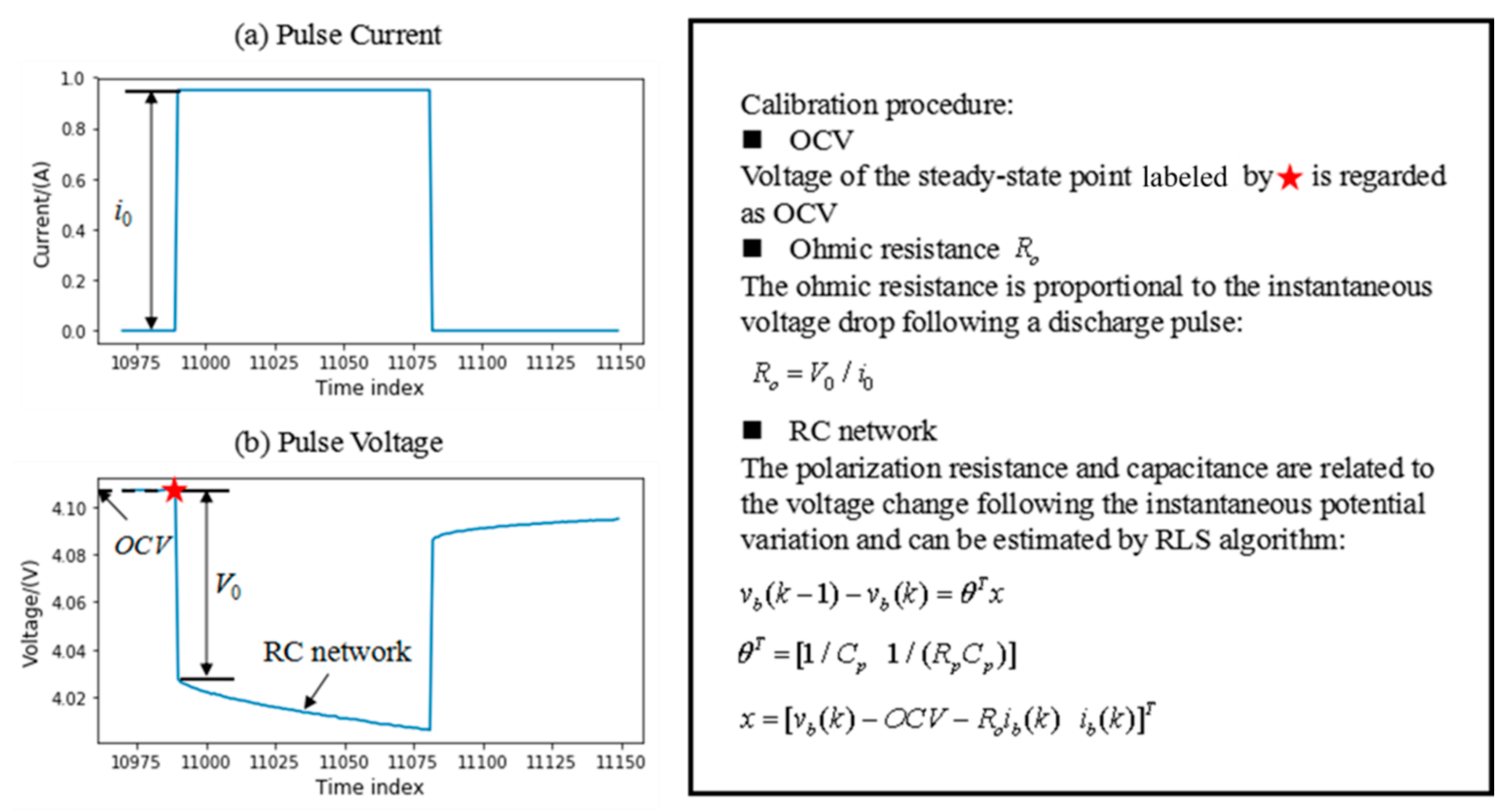
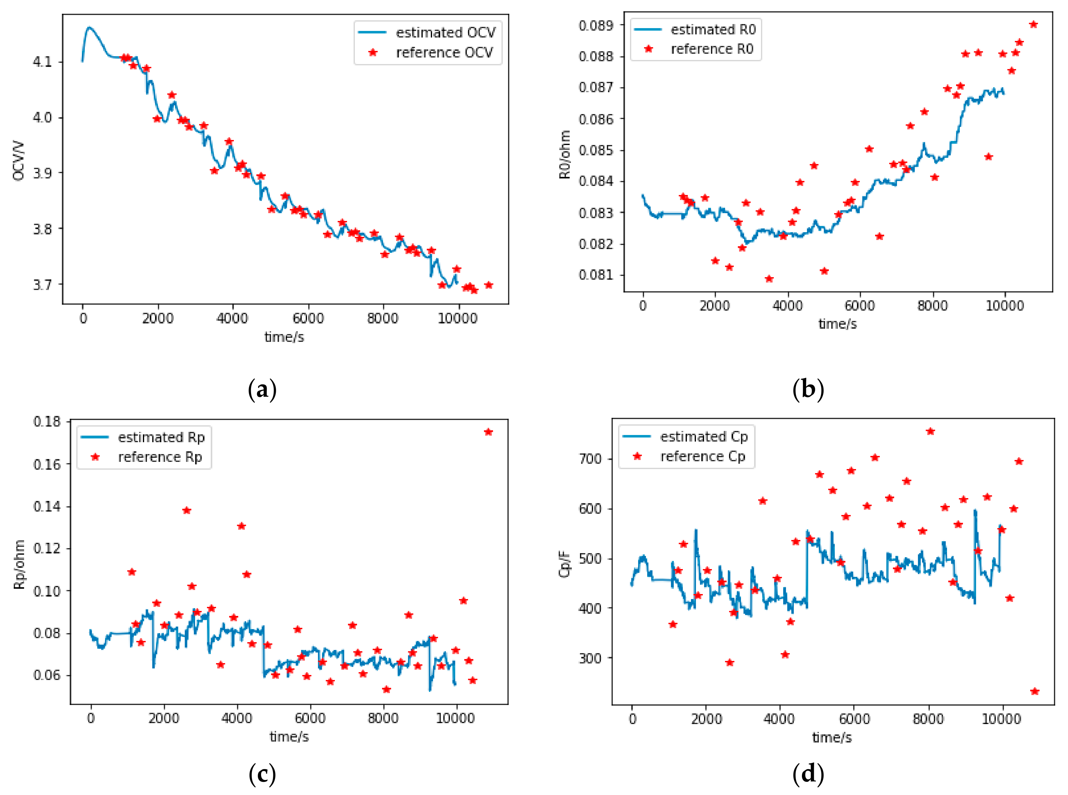
4.1. Verification of Parameter Identification Method

Accurate estimation of the model parameters is significant for the subsequent state estimation [38]. To evaluate the performance of the proposed estimation algorithm, the model parameters calibrated from the HPPC test are worked with as the benchmark. The calibration procedure covers the following three steps, which are shown in Figure 6:

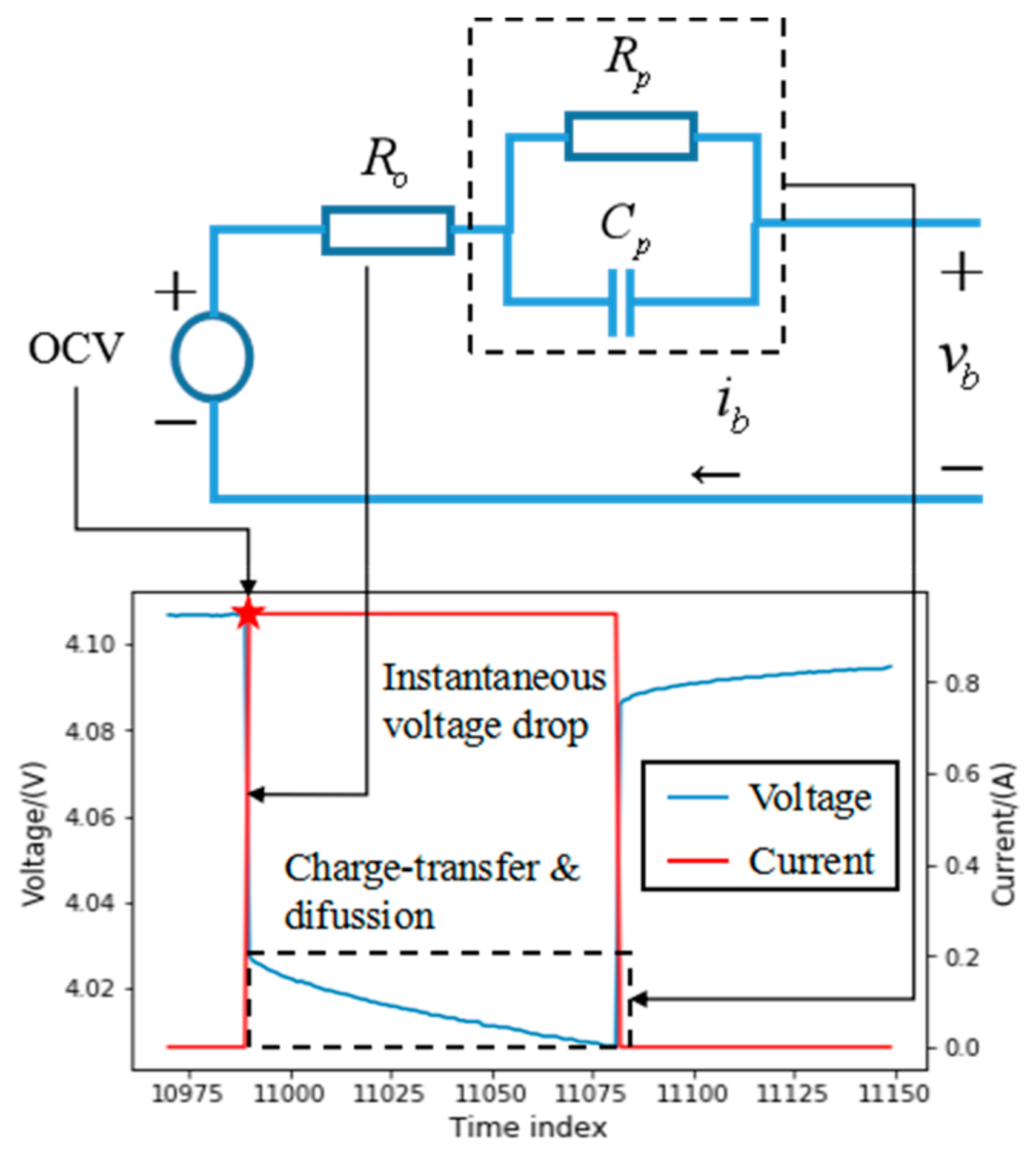
• Take terminal voltage of the steady-state point as OCV.
• Obtain ohmic resistance R_o by dividing the instantaneous voltage drop by the pulse current magnitude.
• Obtain the polarization resistance and capacitance according to the slow-changing voltage after the current pulse based on the recursive least square (RLS) algorithm.

A more detailed description of the calibration method for the HPPC test is available in Ref. [14].

Figure 7 demonstrates the model parameter estimation results for the fresh battery numbered 22 under the HPPC test, together with the calibration values. Generally, the estimated results can follow the trend that the calibration values manifest, which indicates that the proposed linearized battery model and AP algorithm are effective in parameter estimation. It needs to be noticed that the OCV estimation result highly agrees with the calibration value, and the estimation accuracy for ohmic resistance and polarization resistance is also desirable and satisfactory, ensuring subsequent accurate estimation of the battery states. A relatively large derivation between estimated and calibrated values occurs in polarization capacitance estimation when the time index is between around 5000 to 9500. However, just as the sensitivity analysis in Ref. [39] verified, the polarization capacitance has little impact on the SOC estimation, and the estimation error is below 0.5% even when the capacitance value doubles. The following analysis also verifies that the proposed parameter estimation method is reliable in providing accurate state estimation results.

4.2. Verification of SOH Estimation Algorithm

In order to verify the accuracy and adaptability of the proposed SOH estimator, Figure 8a plots the SOH estimation results under HPPC, DST and FUDS tests. It is obvious that the estimated SOH results under three different excitations are close to the real value, which is calibrated by the coulomb counting method. In order to better demonstrate the accuracy of the SOH estimator, Figure 8b gives out the corresponding relative error. It can be seen that the relative error is under 1% for all aging states under three working conditions. The mean relative errors for HPPC, DST and FUDS at different aging levels are 0.51%, 0.46% and 0.39%, respectively, which verifies that the proposed method has desirable accuracy and adaptability performance against different loading profiles under all degradation levels. In addition, considering the slow-varying characteristic of capacity decrease, the SOH estimator does not need to be implemented online. It can be triggered every month offline to calibrate the capacity when the BMS is relatively free. Accurate SOH estimation provides the following SOC and SOP estimators with good estimation bases.

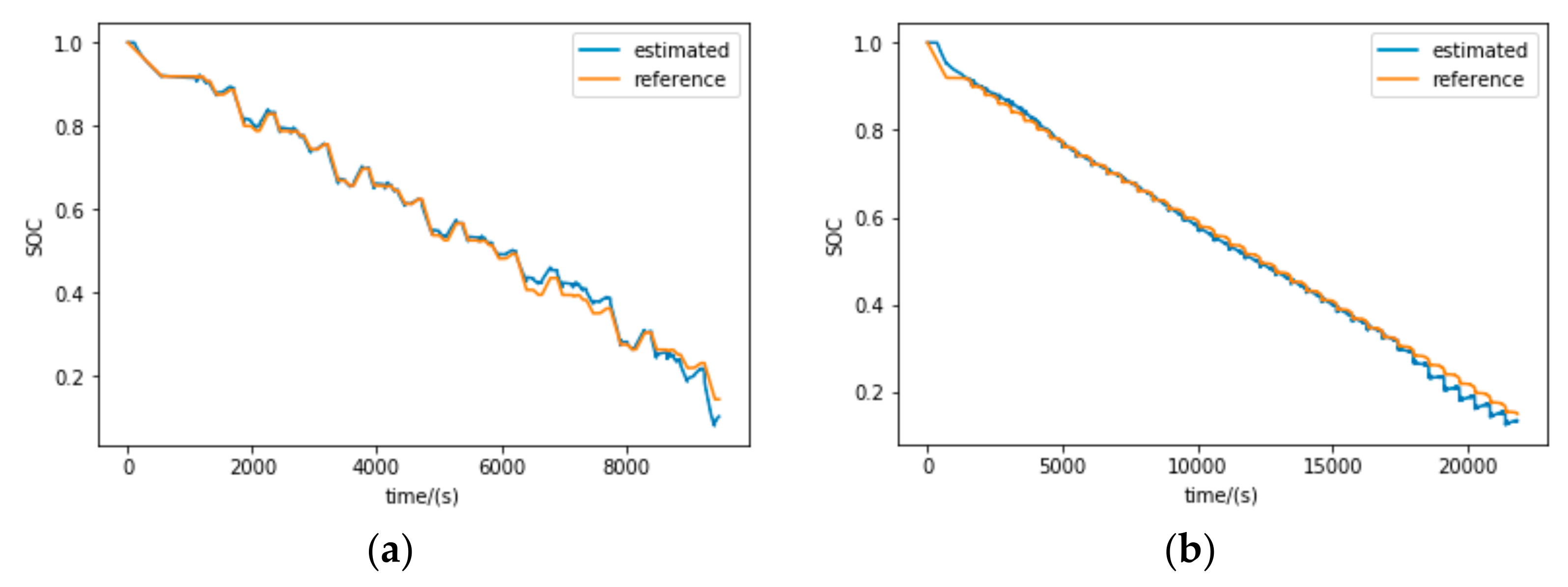
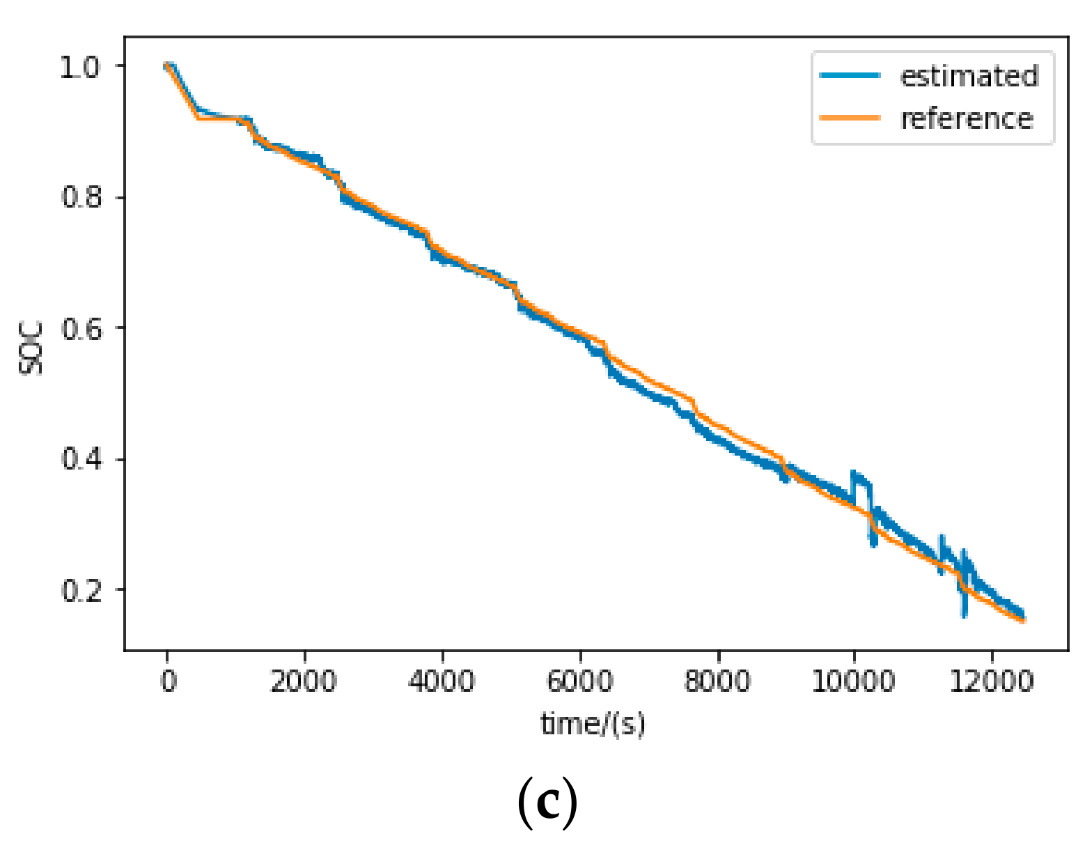
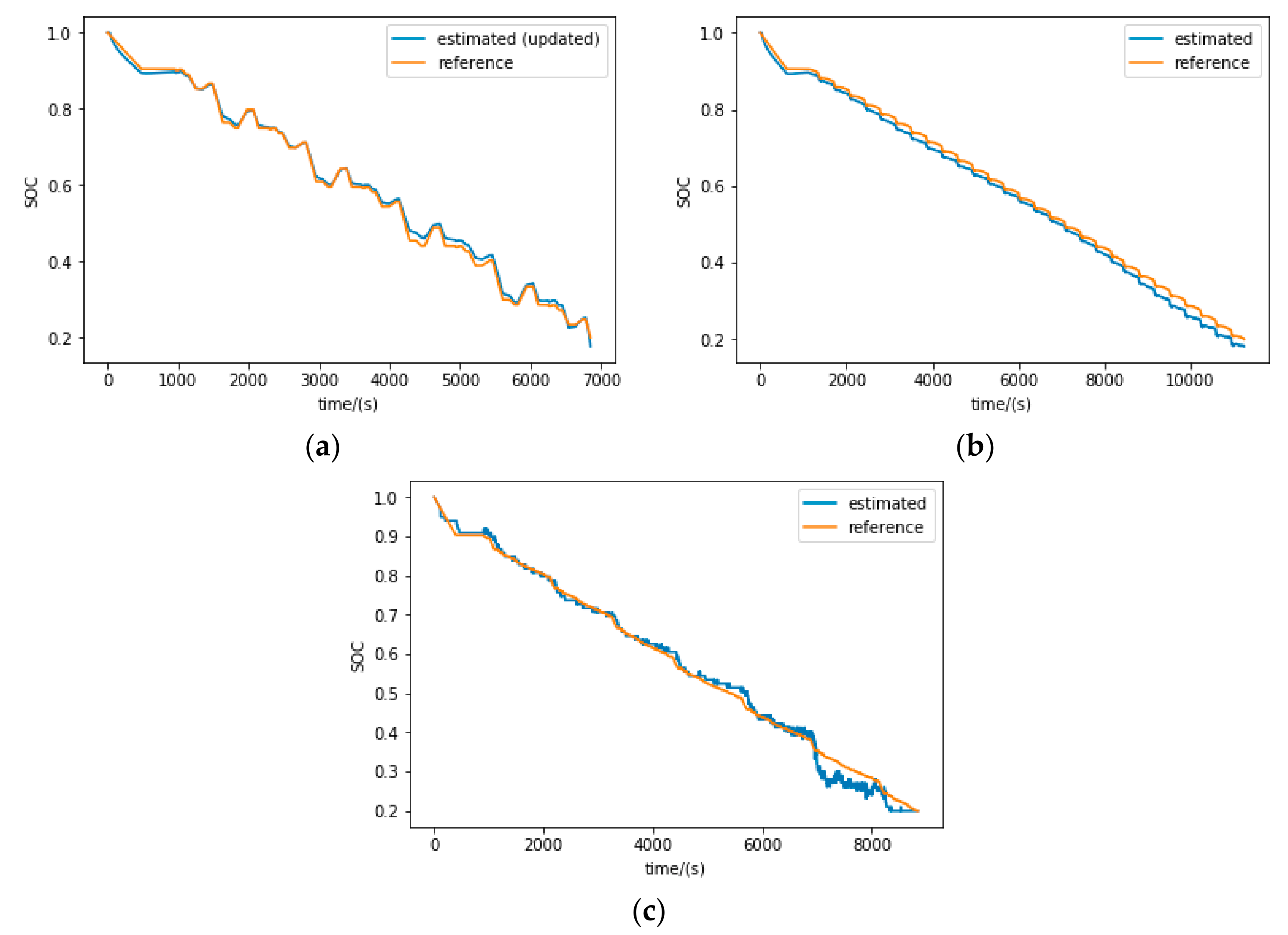
4.3. Verification of SOC Estimation Algorithm

Figure 9 plots the SOC estimation results for the fresh battery under HPPC, DST and FUDS working conditions. According to Figure 9a, the mean estimation error for the fresh battery under the HPPC test when SOC is above 15% is 1.13%. It can be seen that when SOC is above 50%, the estimated SOC is very accurate and the mean estimation error in this range is only 0.51%. However, when SOC drops below 40%, there are some instants when relatively large distinctions exist between the estimated and reference values. This may be caused by the change of battery dynamic proprieties when it is close to the deep discharging state [37]. However, considering the SOC of the battery in electric vehicles rarely drops below 25% and the maximum estimation error when SOC is above 25% is 3.45%, the proposed estimation method is feasible in real-world applications.

Figure 9b,c show that the SOC estimation results under DST and FUDS tests and the mean SOC estimation errors under these two working conditions when SOC is above 15% are 1.04% and 1.31%, respectively. The same phenomenon that the estimated SOC accuracy is desirable in high SOC range and deteriorates in lower SOC range can be observed, with the same reason as explained in the HPPC test above. Generally, the satisfactory performance of the SOC estimator under HPPC, DST and FUDS tests verifies its robustness to different working conditions.

In order to verify the robustness of the proposed method to different aging states, the SOC estimator is applied to the battery after 744 aging cycles and the estimation results are shown in Figure 10. Thanks to the online parameter estimation based on the AP algorithm and update of the battery capacity from the SOH estimator, the SOC estimation error under HPPC, DST and FUDS tests when SOC is above 20% are 0.90%, 1.56% and 1.35%, respectively.

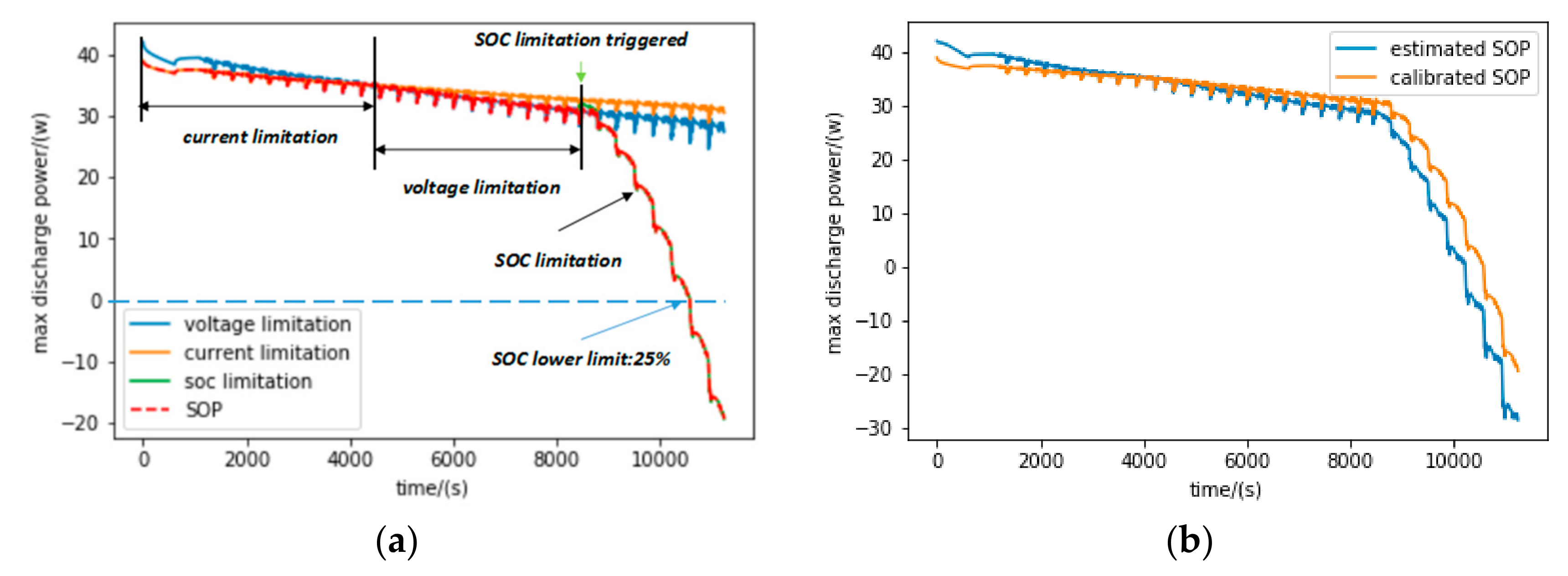
4.4. Verification of SOP Estimation Algorithm

According to Refs. [36,40], to measure battery SOP under the voltage limitation, one can interrupt a standard cycling process by setting the battery voltage to the upper and lower limitations and then monitor the battery current. The maximum discharging and charging capabilities can be obtained by multiplying the measured current by the threshold value of the battery voltage. Similarly, to measure the battery SOP under the current limitation, the current should be set to threshold values and the voltage can be measured. The multiplication of the current threshold and measured voltage is the peak power under current constraints. For SOP under SOC limitation, it can be viewed as an extension of SOP under current limitations, as Equations (31) and (32) transform the SOC constraints to current constraints and the remaining calculation procedure for SOC constraints is the same as that for current limitations. Therefore, in the validation part, attention is paid to SOP under current and voltage limitations, while SOP under SOC limitations can be verified indirectly from current limitations.

Because the battery experiment described in Section 3 does not incorporate the above SOP test procedure, we use the battery model with parameters identified based on the HPPC test to simulate the above test process. Therefore, the accuracy of the battery model is significant for SOP validation. Figure 11 plots the voltage response of the identified battery model (Number 20, fresh) against the measured values. Overlap of the real and simulated voltage response indicates that the identified model is very accurate. The absolute mean voltage errors under HPPC, DST and FUDS tests are 13.41, 9.40 and 9.46 mV, respectively.

The SOP given by simulated experiments and the proposed SOP estimator under discharging and charging situations are shown in Figure 12. For the discharging simulation, the initial SOC is set to 0.3, the voltage and current limitations are set to 2.5 V and 4.7 A, respectively. For the charging situation, the initial SOC is set to 0.9, the voltage and current limitations are set as 4.2 V and −2.35 A, respectively. The closeness between the estimated SOP and the reference value in Figure 12 validates the effectiveness of the proposed SOP estimator.

From Figure 12a,b, it can be seen that the maximum discharging power under voltage and current limitations both decrease as the discharging process continues. The reason is the decreasing OCV accompanied by the lower SOC, which causes the current corresponding to the lower cut-off voltage in Equation (23) and the voltage corresponding to the maximum discharging current in Equation (27) to decrease, resulting in lower SOP as indicated by Equations (25) and (29). However, in the discharging situation, the absolute value of maximum discharging power decreases under voltage limitation while increases under current limitation. It can be explained by the fact that as the charging process continues, the OCV gets closer to the upper cut-off voltage and the permitted charging current under voltage limitations decreases as indicated by Equation (24), leading to diminishing SOP. While under current limitations, increasing the OCV results in higher terminal voltage as indicated by Equation (28), which causes higher SOP as the discharging process continues.

For a better understanding of the three different limitations’ influence on SOP, Figure 11a plots the maximum discharge power constrained by voltage, current and SOC limitations respectively, together with the final SOP determined by all the above constraints. The test is simulated based on the battery model derived from the HPPC test of the battery after 744 aging cycles. It can be seen that, at first, the SOP is determined by current limitation as SOC and voltage at this time are far away from their corresponding lower cut-off value. After about 4000 s, SOP turns out to be determined by voltage limitation as the OCV decreases. When the discharging process further continues, the SOC limitation is triggered and becomes dominant in deciding the final SOP. As SOC decreases to the lower cut-off value, the SOP becomes negative as labeled in Figure 13a. Figure 13b compares the estimated SOP based on the proposed method and the calibrated SOP derived from the battery model. In general, the estimated SOP can track the calibrated value well. The absolute mean error of SOP estimation is 2.69 W. The SOP estimation error at a higher SOC range is mainly caused by the parameter estimation error and is relatively small when current and voltage limitations dominate the SOP value. When SOC limitation is triggered, the SOP estimation error becomes larger as SOC estimation is less accurate when the battery is in the deep discharging state. Because the estimated SOC is lower than its true value after around 8000 s (as shown in Figure 10b), the estimated SOP is correspondingly lower than the calibrated value.

5. Conclusions

This paper presents a systematic framework of SOC, SOH and SOP co-estimation for battery packs used in EVs. The SOH estimator, which is based on the three-dimensional response surface model of OCV and PSO algorithms, is triggered every month when BMS is relatively free to conduct SOH estimation offline. Then, the SOC estimator utilizes the updated capacity and model parameters given by the AP algorithm to estimate the SOC online. At last, the SOP estimator takes advantage of the information provided by the SOH and SOC estimators to give the maximum charging and discharging power considering current, voltage and SOC limitations. Experiments demonstrate that the relative error of the SOH estimator is under 1% under all aging states whatever the loading profile is. The mean absolute SOC estimation error is under 1.6% even when the battery undergoes 744 aging cycles. The SOP estimator is validated by means of the calibrated battery model based on the HPPC test and its performance is ideal.

However, the proposed method heavily relies on the constructed three-dimensional response surface model, both in robustness and accuracy. If the proposed method is to be applied to a battery with different chemical components, the model needs to be reconstructed based on laborious and time-consuming aging experiments of the target battery cell. In addition, the method is only verified under normal room temperature on the cell level. Its effectiveness under different temperatures and on the vehicle level is still in question. In our future work, we mean to propose an adaptive model that has looser requirements for the volume of aging data and verify the proposed method in a wider temperature range on the vehicle level. Moreover, we will compare our method to other existing advanced approaches comprehensively so as to verify that the systematic co-estimation method has better generalization capability and accuracy.

References

1. Guo, N.; Zhang, X.; Zou, Y.; Lenzo, B.; Zhang, T. A Computationally Efficient Path-Following Control Strategy of Autonomous Electric Vehicles with Yaw Motion Stabilization. IEEE Trans. Transp. Electrif. 2020, 6, 728–739. [Google Scholar] [CrossRef]
2. Guo, N.; Zhang, X.; Zou, Y.; Lenzo, B.; Zhang, T.; Göhlich, D. A fast model predictive control allocation of distributed drive electric vehicles for tire slip energy saving with stability constraints. Control. Eng. Pract. 2020, 102, 104554. [Google Scholar] [CrossRef]
3. Zhang, X.; Guo, L.; Guo, N.; Zou, Y.; Du, G. Bi-level Energy Management of Plug-in Hybrid Electric Vehicles for Fuel Economy and Battery Lifetime with Intelligent State-of-charge Reference. J. Power Sources 2021, 481, 228798. [Google Scholar] [CrossRef]
4. Rehman, S.; Khan, K.; Zhao, Y.; Hou, Y. Nanostructured cathode materials for lithium–sulfur batteries: Progress, challenges and perspectives. J. Mater. Chem. A 2017, 5, 3014–3038. [Google Scholar] [CrossRef]
5. Available online: https://www.chyxx.com/industry/202103/936163.html (accessed on 15 April 2021).
6. Mehmood, K.; Iftikhar, Y.; Chen, S.; Amin, S.; Manzoor, A.; Pan, J. Analysis of Inter-Temporal Change in the Energy and CO2 Emissions Efficiency of Economies: A Two Divisional Network DEA Approach. Energies 2020, 13, 3300. [Google Scholar] [CrossRef]
7. Ghosh, A. Possibilities and Challenges for the Inclusion of the Electric Vehicle (EV) to Reduce the Carbon Footprint in the Transport Sector: A Review. Energies 2020, 13, 2602. [Google Scholar] [CrossRef]
8. Wen, G.; Rehman, S.; Tranter, T.G.; Ghosh, D.; Chen, Z.; Gostick, J.T.; Pope, M.A. Insights into Multiphase Reactions during Self-Discharge of Li-S Batteries. Chem. Mater. 2020, 32, 4518–4526. [Google Scholar] [CrossRef]
9. Bhattacharjee, A.; Mohanty, R.; Ghosh, A. Design of an Optimized Thermal Management System for Li-ion Batteries under Different Discharging Conditions. Energies 2020, 13, 5695. [Google Scholar] [CrossRef]
10. Guo, N.; Lenzo, B.; Zhang, X.; Zou, Y.; Zhai, R.; Zhang, T. A Real-Time Nonlinear Model Predictive Controller for Yaw Motion Optimization of Distributed Drive Electric Vehicles. IEEE Trans. Veh. Technol. 2020, 69, 4935–4946. [Google Scholar] [CrossRef] [Green Version]
11. Zou, Y.; Guo, N.; Zhang, X. An integrated control strategy of path following and lateral motion stabilization for autonomous distributed drive electric vehicles. Proc. Inst. Mech. Eng. Part D J. Automob. Eng. 2021, 235, 1164–1179. [Google Scholar] [CrossRef]
12. Li, Y.; Wang, C.; Gong, J. A multi-model probability SOC fusion estimation approach using an improved adaptive unscented Kalman filter technique. Energy 2017, 141, 1402–1415. [Google Scholar] [CrossRef]
13. Xue, Q.; Li, G.; Zhang, Y.; Shen, S.; Chen, Z.; Liu, Y. Fault diagnosis and abnormality detection of lithium-ion battery packs based on statistical distribution. J. Power Sources 2021, 482, 228964. [Google Scholar] [CrossRef]
14. He, W.; Pecht, M.; Flynn, D.; Dinmohammadi, F. A Physics-Based Electrochemical Model for Lithium-Ion Battery State-of-Charge Estimation Solved by an Optimised Projection-Based Method and Moving-Window Filtering. Energies 2018, 11, 2120. [Google Scholar] [CrossRef] [Green Version]
15. Goh, T.; Park, M.; Seo, M.; Kim, J.G.; Kim, S.W. Capacity estimation algorithm with a second-order differential voltage curve for Li-ion batteries with NMC cathodes. Energy 2017, 135, 257–268. [Google Scholar] [CrossRef]
16. Einhorn, M.; Conte, F.V.; Kral, C.; Fleig, J. A Method for Online Capacity Estimation of Lithium Ion Battery Cells Using the State of Charge and the Transferred Charge. IEEE Trans. Ind. Appl. 2011, 48, 736–741. [Google Scholar] [CrossRef]
17. Plett, G. High-Performance Battery-Pack Power Estimation Using a Dynamic Cell Model. IEEE Trans. Veh. Technol. 2004, 53, 1586–1593. [Google Scholar] [CrossRef] [Green Version]
18. Malysz, P.; Ye, J.; Gu, R.; Yang, H.; Emadi, A. Battery State-of-Power Peak Current Calculation and Verification Using an Asymmetric Parameter Equivalent Circuit Model. IEEE Trans. Veh. Technol. 2015, 65, 4512–4522. [Google Scholar] [CrossRef]
19. Waag, W.; Fleischer, C.; Sauer, D.U. Adaptive on-line prediction of the available power of lithium-ion batteries. J. Power Sources 2013, 242, 548–559. [Google Scholar] [CrossRef]
20. Zou, Y.; Hu, X.; Ma, H.; Li, S.E. Combined State of Charge and State of Health estimation over lithium-ion battery cell cycle lifespan for electric vehicles. J. Power Sources 2015, 273, 793–803. [Google Scholar] [CrossRef]
21. Dong, G.; Wei, J.; Chen, Z. Kalman filter for onboard state of charge estimation and peak power capability analysis of lithium-ion batteries. J. Power Sources 2016, 328, 615–626. [Google Scholar] [CrossRef]
22. Zheng, L.; Zhang, L.; Zhu, J.; Wang, G.; Jiang, J. Co-estimation of state-of-charge, capacity and resistance for lithium-ion batteries based on a high-fidelity electrochemical model. Appl. Energy 2016, 180, 424–434. [Google Scholar] [CrossRef]
23. Sun, F.; Xiong, R.; He, H. Estimation of state-of-charge and state-of-power capability of lithium-ion battery considering varying health conditions. J. Power Sources 2014, 259, 166–176. [Google Scholar] [CrossRef]
24. Shen, P.; Ouyang, M.; Lu, L.; Li, J.; Feng, X. The Co-estimation of State of Charge, State of Health, and State of Function for Lithium-Ion Batteries in Electric Vehicles. IEEE Trans. Veh. Technol. 2017, 67, 92–103. [Google Scholar] [CrossRef]
25. Gonzalez, A.; Ferrer, M.; Albu, F.; de Diego, M. Affine Projection Algorithms: Evolution to Smart and Fast Algorithms and Applications. In Proceedings of the 20th European Signal Processing Conference (EUSIPCO), Bucharest, Romania, 27–31 August 2012; pp. 1965–1969. [Google Scholar]
26. Sun, F.; Xiong, R. A novel dual-scale cell state-of-charge estimation approach for series-connected battery pack used in electric vehicles. J. Power Sources 2015, 274, 582–594. [Google Scholar] [CrossRef]
27. Yang, R.; Xiong, R.; He, H.; Mu, H.; Wang, C. A novel method on estimating the degradation and state of charge of lithium-ion batteries used for electrical vehicles. Appl. Energy 2017, 207, 336–345. [Google Scholar] [CrossRef]
28. Guo, N.; Zhang, X.; Zou, Y.; Guo, L.; Du, G. Real-time predictive energy management of plug-in hybrid electric vehicles for coordination of fuel economy and battery degradation. Energy 2021, 214, 119070. [Google Scholar] [CrossRef]
29. Guo, N.; Shen, J.; Xiao, R.; Yan, W.; Chen, Z. Energy management for plug-in hybrid electric vehicles considering optimal engine ON/OFF control and fast state-of-charge trajectory planning. Energy 2018, 163, 457–474. [Google Scholar] [CrossRef]
30. Duong, V.-H.; Bastawrous, H.A.; Lim, K.; See, K.W.; Zhang, P.; Dou, S.X. Online state of charge and model parameters estimation of the LiFePO4 battery in electric vehicles using multiple adaptive forgetting factors recursive least-squares. J. Power Sources 2015, 296, 215–224. [Google Scholar] [CrossRef]
31. Venter, G.; Jaroslaw, S.S. Particle Swarm Optimization. AIAA J. 2003, 41, 129–132. [Google Scholar] [CrossRef] [Green Version]
32. Gao, D.; Huang, M. Prediction of Remaining Useful Life of Lithium-ion Battery based on Multi-kernel Support Vector Machine with Particle Swarm Optimization. J. Power Electron. 2017, 17, 1288–1297. [Google Scholar]
33. Andre, D.; Appel, C.; Soczka-Guth, T.; Sauer, D.U. Advanced mathematical methods of SOC and SOH estimation for lithium-ion batteries. J. Power Sources 2013, 224, 20–27. [Google Scholar] [CrossRef]
34. Gao, W.; Zou, Y.; Sun, F.; Hu, X.; Yu, Y.; Feng, S. Data pieces-based parameter identification for lithium-ion battery. J. Power Sources 2016, 328, 174–184. [Google Scholar] [CrossRef]
35. Lu, L.; Han, X.; Li, J.; Hua, J.; Ouyang, M. A review on the key issues for lithium-ion battery management in electric vehicles. J. Power Sources 2013, 226, 272–288. [Google Scholar] [CrossRef]
36. Feng, T.; Yang, L.; Zhao, X.; Zhang, H.; Qiang, J. Online identification of lithium-ion battery parameters based on an improved equivalent-circuit model and its implementation on battery state-of-power prediction. J. Power Sources 2015, 281, 192–203. [Google Scholar] [CrossRef]
37. Hu, X.; Li, S.; Peng, H. A comparative study of equivalent circuit models for Li-ion batteries. J. Power Sources 2012, 198, 359–367. [Google Scholar] [CrossRef]
38. Hu, X.; Li, S.; Peng, H.; Sun, F. Robustness analysis of State-of-Charge estimation methods for two types of Li-ion batteries. J. Power Sources 2012, 217, 209–219. [Google Scholar] [CrossRef]
39. Sepasi, S.; Ghorbani, R.; Liaw, B.Y. A novel on-board state-of-charge estimation method for aged Li-ion batteries based on model adaptive extended Kalman filter. J. Power Sources 2014, 245, 337–344. [Google Scholar] [CrossRef]
40. Wang, S.; Verbrugge, M.; Wang, J.S.; Liu, P. Power prediction from a battery state estimator that incorporates diffusion resistance. J. Power Sources 2012, 214, 399–406. [Google Scholar] [CrossRef]
Figure 1. The scheme of the co-estimation algorithm.
Sustainability 13 05166 g001
Figure 2. First-order RC ECM together with corresponding HPPC response.
Sustainability 13 05166 g002
Figure 3. The three-dimensional response surface model of OCV.
Sustainability 13 05166 g003
Figure 4. The framework of the proposed SOH estimator.
Sustainability 13 05166 g004
Figure 5. The proposed SOP estimation algorithm.
Sustainability 13 05166 g005
Figure 6. Parameter calibration procedure for HPPC test.
Sustainability 13 05166 g006
Figure 7. Parameter identification results of the proposed method. (a) OCV; (b) ohmic resistance; (c) polarization resistance; (d) polarization capacitance.
Sustainability 13 05166 g007
Figure 8. Capacity estimation results at different aging states under different working conditions. (a) Capacity; (b) Relative error.
Sustainability 13 05166 g008
Figure 9. SOC estimation results of the fresh battery under different working conditions. (a) HPPC; (b) DST; (c) FUDS.
Sustainability 13 05166 g009aSustainability 13 05166 g009b
Figure 10. SOC estimation results of the aged battery under different working conditions. (a) HPPC; (b) DST; (c) FUDS.
Sustainability 13 05166 g010
Figure 11. Verification of the battery model accuracy. (a) HPPC; (b) DST; (c) FUDS.
Sustainability 13 05166 g011
Figure 12. SOP for discharging under (a) voltage limitation and (b) current limitation and SOP for charging under (c) voltage limitation and (d) current limitation.
Sustainability 13 05166 g012
Figure 13. SOP for discharging under DST test. (a) Interaction of different limitations; (b) Comparison of estimated and calibrated SOP.
Sustainability 13 05166 g013