3.2.2. Independent Variables
In order to verify the hypothesis proposed in this article, it should be considered that whether farmers are willing to save water is also largely affected by their evaluation of the irrigation-water-saving potential. If the farmers believe that it does not have any water-saving potential, then the explicit subsidy plan proposed in this article will not be able to stimulate them to save water. Therefore, this paper selects the intersection of farmers’ loss aversion and water-saving potential as the main independent variable.
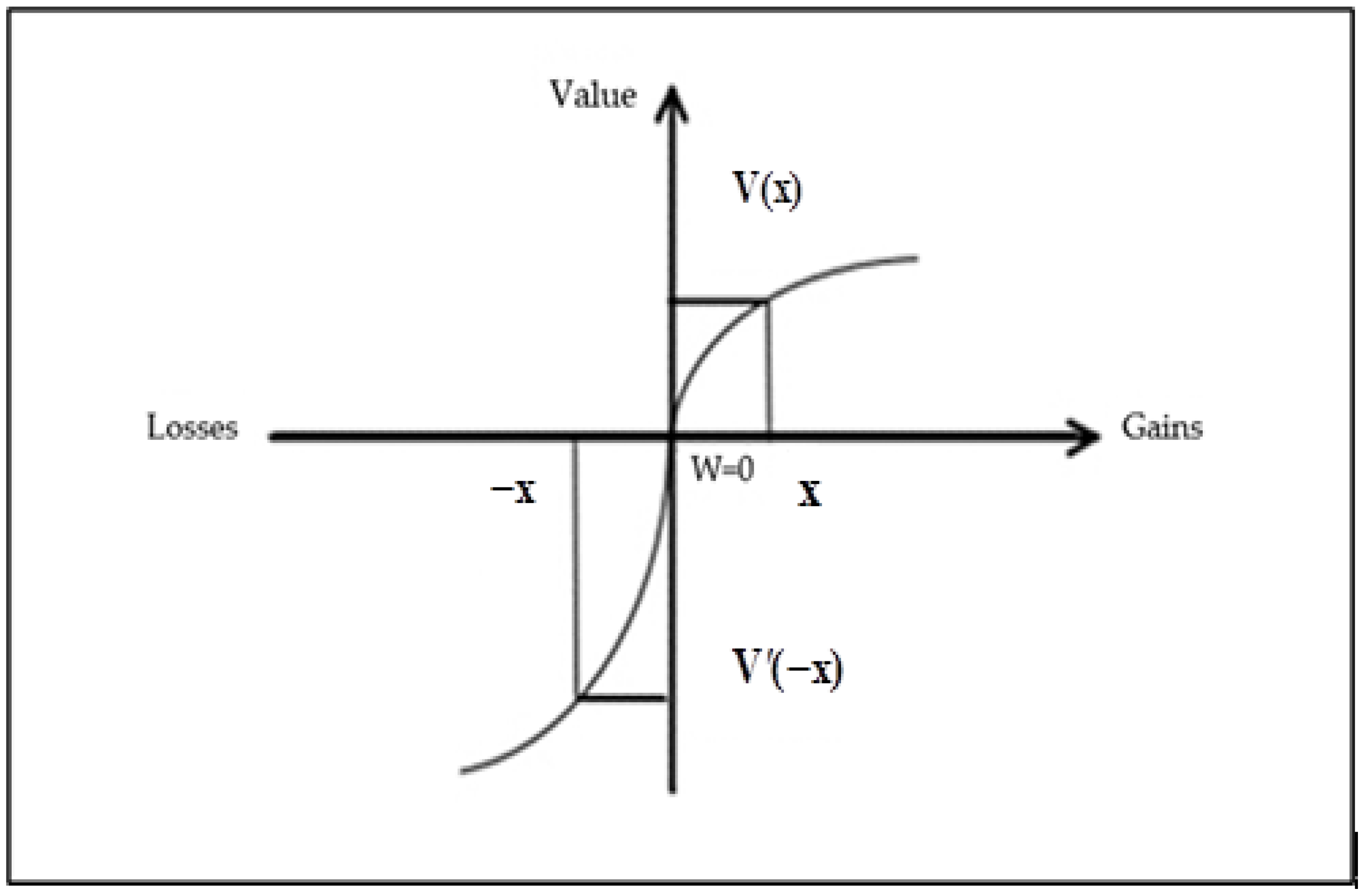
The loss aversion in the article is measured by the following question: “If another farmer wants to buy your water, what is the lowest price you accept to sell your water (WTA)? If there is water that can be bought, what is the highest water price you are willing to pay (WTP)?” The ratio of the two (WTA/WTP) was used as the subject’s degree of loss aversion.
The reason we asked this question was to make a similar situation to the endowment effect experiment without risk [
28], and elicit WTA and WTP from the same individual. The gap between WTA and WTP can be interpreted as evidence for loss aversion in riskless choice. According to the results, all farmers were divided into two categories: 0 = no loss aversion (WTA/WTP ≤ 1), 1 = loss aversion (WTA/WTP > 1). The statistical results are shown in
Table 2.
Most documents have confirmed the widespread existence of loss aversion, but our results show that only close to 1/3 of the interviewed farmers have loss aversion. This may be related to the imperfect market of local agricultural irrigation water rights. Water is a special commodity. It is not a fully market-oriented commodity, so the measurement results may only partially reflect the preferences of farmers.
The water-saving potential of farmers is measured by asking farmers to answer the question “In general, do you think your irrigation water has water-saving potential?” Options 1–5 indicate “no potential at all”, “almost no potential”, “balanced”, “some potential”, and “big potential”, respectively. The statistical results are shown in
Table 3.
To further observe the impact of loss aversion on the water-saving effect of the explicit subsidy, this paper introduces two interaction terms. The first one is equal to loss aversion (0 = no loss aversion (WTA/WTP ≤ 1), 1 = loss aversion (WTA/WTP > 1)) multiplied by the evaluation of the water-saving potential of farmers, which means the level of water-saving potential considered by farmers with loss aversion; the second one is equal to no loss aversion (1 = no loss aversion (WTA/WTP ≤ 1), 0 = Loss aversion (WTA/WTP > 1)) multiplied by the evaluation of the water-saving potential of farmers, which means the level of water-saving potential considered by farmers without loss aversion. Interaction term 1 and term 2 are designed to isolate farmers who have (no) loss aversion, and observe their perception of water-saving potential and the impact of loss aversion on the dependent variable.
According to the above classification, the sample households can be roughly divided into four groups: households with both loss aversion and water-saving potential, households with only loss aversion but no water-saving potential, households without loss aversion but with water-saving potential, and households without either loss aversion or water-saving potential.
3.2.3. Control Variables
Combining existing literature [
34,
39,
40,
41], this paper selects three types of variables as the control variables: household head characteristics, family characteristics, and regional differences.
Age: Generally speaking, the older the household heads are, the richer their agricultural production experiences, and the more they are inclined to save water to reduce agricultural production costs. Younger household heads with insufficient production experiences may increase irrigation water to ensure yield. Therefore, it is expected that age will have a positive effect on the incentives for water-saving.
Years of education: The level of farmers’ understanding of the new policy is related to their education. The higher the level of education, the stronger the ability to understand and accept new things. On the whole, education level should have a positive impact on the incentives for saving-water.
Health status: A dichotomous variable is used to reflect the health status of farmers, where 1 = good, and 0 = fair or poor. Farmers with better health will have more energy and have more advantages in agricultural production. Compared with unhealth farmers, they are more inclined to save water, thereby saving agricultural production costs. It is expected that their health status will have a positive impact on the incentives for water-saving.
Identity: A dichotomous variable is used here to reflect the identity of the head of household. Party members or cadres in the village (or both) are the promoters of the implementation of the new policy, and their awareness of the new policy is higher than normal farmers.
Risk preference: We use a question to measure farmers’ risk preference. Farmers have two choices: option A is the opportunity to get 100 RMB for sure (without risk); and option B, a simple lottery with a 50% chance of getting more than 100 RMB (an amount that gradually increases from 150 RMB to 1500 RMB) and a 50% chance of getting nothing, as shown in
Table 4.
When the expected value of option B is small, the farmers will tend to choose the risk-free option A. As the possible benefits of option B increase, farmers will start to choose B at a certain amount, and will continue to choose B thereafter. For most of the farmers, we can observe this turning point from option A to B, which can be used to measure the level of risk aversion. We employed a simple way to calculate the risk aversion index of farmers, as shown below:
Risk aversion index = 1—the number of option B was chose/8
This is an inverse indicator. The larger the number of option B, the more risk-averse the farmer is, and the smaller the index. For example, the index will equal 1 if a farmer always chooses the riskless option A, which means an extremely loss-averse person. The larger the index, the more risk-preferring the farmer is. For example, the index will equal 0 if the farmer always chooses option B, meaning a risk-seeking farmer who loves risk. Previous research shows that farmers with an appetite for risk are more willing to try new technologies [
42], and they are more receptive to new things. It is expected that the explicit subsidy program will provide water-saving incentives for risk-preferring farmers.
Water price judgment: Farm households are divided into three categories based on their water price judgments: the first category is farmers who believe that the current water price is higher than the cost of water supply; the second category is farmers who believe that the current water price is lower than the water supply cost; the third category is farmers who think that water price is similar to the cost of water supply. This article takes the third category as a reference and introduces two dummy variables to observe whether the explicit subsidy plan will have different water-saving incentives for the three kinds of farmers with different water price judgments.
Canal evaluation: The quality of the irrigation canal directly reflects the quality of the water supply for farmers. The better the channel, the higher the irrigation efficiency of farmers, the less water wasted during the irrigation process, and the greater the potential for farmers to save water. It is expected that the better the canal evaluation, the more significant the water-saving incentives provided by explicit subsidy will be.
Cultivated land area: Generally speaking, the larger the area of arable land, the more favorable it is for large-scale agricultural production to achieve economies of scale and reduce agricultural production costs. Farmers with a larger area of arable land are more inclined to adopt advanced agricultural production technologies [
43], which also means more room for water-saving. Therefore, it is assumed that the area of arable land has a positive effect on the water-saving incentives.
Planting structure: the proportion of the sown area of cash crops to the total sown area. The larger the proportion of cash crops, the more farmers will increase their water consumption to ensure profits. Although the explicit subsidy program can help active farmers save water costs, for those with a large proportion of cash crops, they are not motivated to save water in order to ensure yield.
Irrigation water used: Total water consumption per mu. Farmers who used too much irrigation water have insufficient water-saving awareness and insufficient planting experience. The water-saving space of these farmers is larger than that of farmers who used less irrigation water. Therefore, under the stimulation of the explicit subsidy program, farmers who used more irrigation water will be more motivated to save water.
Greenhouse: Farmers were asked whether they had used a greenhouse in 2012, which is a dichotomous variable. This variable is used to reflect the ability of farmers to accept new things and new technologies. Farmers who use greenhouses are more able to accept the implementation of the explicit subsidy program, which can promote farmers to save more water.
There are differences in the natural environment of the three inland river basins. First, there are differences within the same watershed. Differences in elevation, precipitation, temperature, and evaporation in the upper, middle, and lower reaches of the river lead to differences in the supply of surface water and groundwater. Second, there are differences between the river basins. The three river basins run from east to west. As rainfall has decreased and evaporation has increased, the degree of drought has gradually increased, and the water demand of crops has also increased accordingly. Third, the human environment of the river basins is different. The population density of the three river basins gradually decreases from east to west, and the per capita arable land area and irrigation quota per unit of arable land increases. The above-mentioned differences will more or less interact and affect the views of farmers in the basin on the use of irrigation water, and the water-saving incentives. However, because these influencing factors are difficult to separate and refine in one survey, many factors interact with each other. Therefore, all the independent variable factors not mentioned above are integrated into regional difference factors and included as an influencing variable in the regression analysis. Shiyang River basin was taken as the reference area, and two dummy variables of Hei and Shule River were introduced to compare with it.
A specific description of the variables is shown in
Table 5.


