Article

Contrasting Influences of Seasonal and Intra-Seasonal Hydroclimatic Variabilities on the Irrigated Rice Paddies of Northern Peninsular Malaysia for Weather Index Insurance Design

by
Zed Zulkafli
1,*,
Farrah Melissa Muharam
2,*,
Nurfarhana Raffar
1,
Amirparsa Jajarmizadeh
1,
Mukhtar Jibril Abdi
1,
Balqis Mohamed Rehan
1 and
Khairudin Nurulhuda
3
1
Department of Civil Engineering, Faculty of Engineering, Universiti Putra Malaysia, UPM Serdang 43400, Malaysia
2
Department of Agriculture Technology, Faculty of Agriculture, Universiti Putra Malaysia, UPM Serdang 43400, Malaysia
3
Department of Biological and Agricultural Engineering, Faculty of Engineering, Universiti Putra Malaysia, UPM Serdang 43400, Malaysia
*
Authors to whom correspondence should be addressed.
Sustainability 2021, 13(9), 5207; https://doi.org/10.3390/su13095207
Submission received: 11 February 2021 / Revised: 9 April 2021 / Accepted: 12 April 2021 / Published: 7 May 2021
(This article belongs to the Special Issue Climate Risk Management for Resilient Agricultural Systems)

Abstract

:
Good index selection is key to minimising basis risk in weather index insurance design. However, interannual, seasonal, and intra-seasonal hydroclimatic variabilities pose challenges in identifying robust proxies for crop losses. In this study, we systematically investigated 574 hydroclimatic indices for their relationships with yield in Malaysia’s irrigated double planting system, using the Muda rice granary as a case study. The responses of seasonal rice yields to seasonal and monthly averages and to extreme rainfall, temperature, and streamflow statistics from 16 years’ observations were examined by using correlation analysis and linear regression. We found that the minimum temperature during the crop flowering to the maturity phase governed yield in the drier off-season (season 1, March to July, Pearson correlation, r = +0.87; coefficient of determination, R2 = 74%). In contrast, the average streamflow during the crop maturity phase regulated yield in the main planting season (season 2, September to January, r = +0.82, R2 = 67%). During the respective periods, these indices were at their lowest in the seasons. Based on these findings, we recommend temperature- and water-supply-based indices as the foundations for developing insurance contracts for the rice system in northern Peninsular Malaysia.

1. Introduction

Rice is the staple food of almost half of the world’s population [1], while almost one fifth depends on the rice industry for their source of employment and livelihoods [2]. The share of rice in South Asia in its total gross domestic product (GDP) accounted for 8.4% in 1961 but had declined to 2.7% in 2007 [3]. Meanwhile, Southeast Asian (SEA) countries have depended on agriculture for their economies and as food sources, with rice contributing 2.3% or 2.4 billion RM of Malaysia’s GDP in 2016 [4].
Many rice producing countries monitor production through self-sufficiency levels (SSL) that indicate the proportion of rice production to rice availability such as imports and stocks. For example, rice importer countries such as the Philippines, Malaysia, and Vietnam have 93%, 70%, and 97% SSL, respectively [4,5]. In the case of Malaysia, the SSL is comparatively low, and rice production has hovered between 60–70% for about 30 years, even with the production having increased over the decades from 1.9 million tonnes in 1990 to 3.5 million tonnes in 2017 [4]. Despite being in the hub of the world’s rice economy, and despite the high market demand, rice production in Malaysia remains low and without monumental efforts being made to tackle major issues such as production loss due to extreme weather events and climate change [6], decreasing cultivation area [7], changing socioeconomic scenarios [8], and increasing production cost. These local issues that affect rice production illustrate common future threats to food security in all rice-consuming and -producing nations.
Nevertheless, in managing risks related to agricultural production, weather index insurance has proven to be an effective tool to increase coping capacity and to sustain productivity. The strategy relies on associations between hydroclimatic variables and crop yields [9,10] and utilises locally developed and highly correlated indices based on these variables as proxies for the negative impacts of weather on crop production [11,12,13]. As a result, measurements of crop damages post extreme climate events become inconsequential, unlike in traditional crop insurance [14]. Commonly used indices are based on rainfall or temperature [15,16,17,18], although combined or mixed indices of rainfall and temperature [19,20,21], and streamflow and reservoir indices [22,23,24] have also been used. These indices can be applied in the form of either surplus or deficit, averages, cumulative amounts, and minima or maxima [18].
Tremendous efforts in the development and implementation of weather index insurance have been made in the agricultural areas of Africa, Latin America, and some parts of Asia, especially as a mechanism of risk transfer [13,25,26]. However, the variabilities of hydroclimatic variables that influence local crop production pose challenges in minimising the basis risk, i.e., the risk of no payment incurred when there is an actual loss in yield, and, conversely, of payment incurred when there is no actual loss [27]. Weather indices must be good indicators of yields, particularly poor yields to minimise basis risk [28].
Hence, increased understanding of the relationship between hydroclimatic variables and rice performances at local scales is vital, given that the next rice industry challenge is related to climate changes and the consequent negative impacts on water resources [9,29,30,31]. A Malaysian framework would be highly relevant, considering that the government heavily subsidises rice production and compensates rice losses due to extreme weather [9,32,33]. Extreme climatic events such as floods and droughts have affected Malaysia’s rice productivity [6,8]. These included the effects of temperature rise and rainfall fluctuations. The 1997–1998 droughts due to the El Niño led to a massive rice yield loss with an associated economic loss of 218 million RM [34,35].
Malaysia also represents an interesting case of an irrigated rice double-planting system, whereby rice cultivation is intensified by irrigation during an off-season. Here, successful implementation of the weather index insurance requires bridging a substantial gap in knowledge related to crop productivity and its response to weather as well as water management strategies. In particular, the seasonal and intra-seasonal influences of various hydroclimatic indices on rice production warrant close inspections due to the contrasting dependence on (1) rainfall in the main planting season and (2) irrigation in the off-season as supplied from the upstream water catchment areas [36].
Considering this, our work, therefore, aimed to address the identified gap by (1) systematically examining the correlation and developing regression models between observed rice crop yields, based on individual and mixed monthly averages and extreme indices derived from hydroclimatic variables such as rainfall, temperature, and streamflow measurements and (2) relating the findings in terms of rice growth stages. The case study, the Muda area rice granary, produces approximately 40 percent of the nation’s rice, and is in a drought- and flood-prone region in the northwest of Peninsular Malaysia. The drought-induced economic losses were estimated to be 10.6–16.3 million RM and 4–6 million RM in the main season and in the off-season, respectively, since 2003–2013 [37], whereas the rice yields were impacted by several flood events in 2003, 2005, and 2017 [38]. In the main season of 2005/2006 alone, floods caused 50,000 MT of yield loss, affecting 10,580 farmers. The susceptibility of the area to extreme weather, combined with its important role in national food security, make the Muda area a suitable test bed for assessing the potential for weather index insurance in the country.

2. Materials and Methods

2.1. Study Area

Malaysia borders Thailand in northern Peninsular Malaysia as well as Indonesian Borneo. It has a total area of 330,800 km2 and a population of 32.68 million in 2019 [39]. Malaysia’s largest rice granary is the Muda area, which produces about 38.8% of the local rice [4]. It is a high-performing area with yields above 5.0 MT/ha due to the government’s provision of extensive infrastructure since the inception of the Muda Irrigation Project. Located in the northwest of Peninsular Malaysia (Figure 1), the Muda area occupies 126,155 ha of land, of which 76% is under paddy cultivation. The granary practices double-planting seasons (Table 1), mostly via direct seeding but also transplanting.
Cultivated paddy in the Muda area is less affected by the northeast (November to February) and the southwest (May to August) monsoons due to the Titiwangsa and Sumatra mountain ranges that block heavy precipitation. During the southwest monsoon, most of the states of the west coast of the peninsula are subjected to a drier period; however, during this monsoon period, the northwest region is wetter than the rest of the country due to less shielding by the Sumatra range [41,42]. In contrast, the area receives heavy rainfall during the two inter-monsoon seasons, approximately around April and October, in the form of convective rains [41,42]. The annual rainfall ranges from 2000 to 3000 mm, while the average temperature is recorded to be around 27 °C [43]. Moreover, higher temperatures during the month of February and March coincide with low rainfall at the tail of the Northeast monsoon period, which typically brings extreme rainfall and floods but on the east coast of the peninsula [41,42]. This results in a drier period at the start of the off-season. Thus, irrigation is required to increase rice production annually.
Here, water resources are comprised of direct rainfall (52%), controlled flows from the Pedu reservoir in the upstream (32%), uncontrolled flows from the catchment areas downstream of the reservoir (10%), and recycled water (6%) [44]. The water demand management follows a specified hierarchy. If direct rainfall is insufficient for ponding, (1) water is sourced directly from uncontrolled flows, provided there is sufficient supply in the river to meet demand. If river supply is insufficient (2), water is recycled from downstream of the paddy field drainage via pumping, and as a final resort (3), water is released from the reservoir. The bulk of the irrigation water demand is for land preparation before wet seeding or transplanting; then, supplementary demand may be required up until 1–2 weeks prior to harvest. During any water crisis, domestic and industrial water demand takes precedence over agricultural demand.

2.2. Data Collection

Rainfall, temperature, streamflow, and yield data covering a period of 16 years from March 2001 to January 2017 were obtained from various sources. Daily accumulated rainfall data were obtained from three rainfall stations operated by the Muda Agricultural Development Authority (MADA) (Station 12 Bt. 4 Sanglang, 24 Gunong Kriang, and 44 Alator Tokal) and one station operated by the Department of Irrigation and Drainage, Malaysia (DID) (Station JPS 6206035) at Kuala Nerang (Figure 1). Henceforth, these four stations would be referred to as MADA12, MADA24, MADA44, and JPS, respectively. Daily minimum and maximum temperature data were retrieved for the Alor Setar (AS) and Chuping (Ch) meteorological stations operated by the Department of Meteorology, Malaysia (DMM). Subsequently, the daily average temperatures were derived based on the average of the minimum and maximum temperatures. Additionally, daily streamflow data at Kuala Nerang station and seasonal rice yield values at the granary scale from both seasons of planting were obtained from MADA.

2.3. Derivation of Average and Extreme Hydroclimatic Indices

Daily rainfall was summarised into average and extreme indices based on the monthly mean, maximum, dry days, and wet days values (Table 2). Similarly, the streamflow-based indices were computed based on the monthly minimum, mean, and maximum values. Daily maximum, mean, and minimum daily temperature data were also aggregated to monthly maximum, minimum, and mean values to comprise the temperature-based indices. To test the timing and seasonality of the hydroclimatic indices and how they relate with yield, for season 1, indices were calculated for the individual months of March, April, May, June, and July; for the mid-season months from April to June (AMJ); and for the entire season (March to July, or MAMJJ). Likewise, indices were calculated for season 2 for the individual months of September, October, November, December, and January; for the mid-season months from October to December (OND); and for the entire season (September to January, or SONDJ). In total, there are 287 indices investigated per season and 574 indices overall.

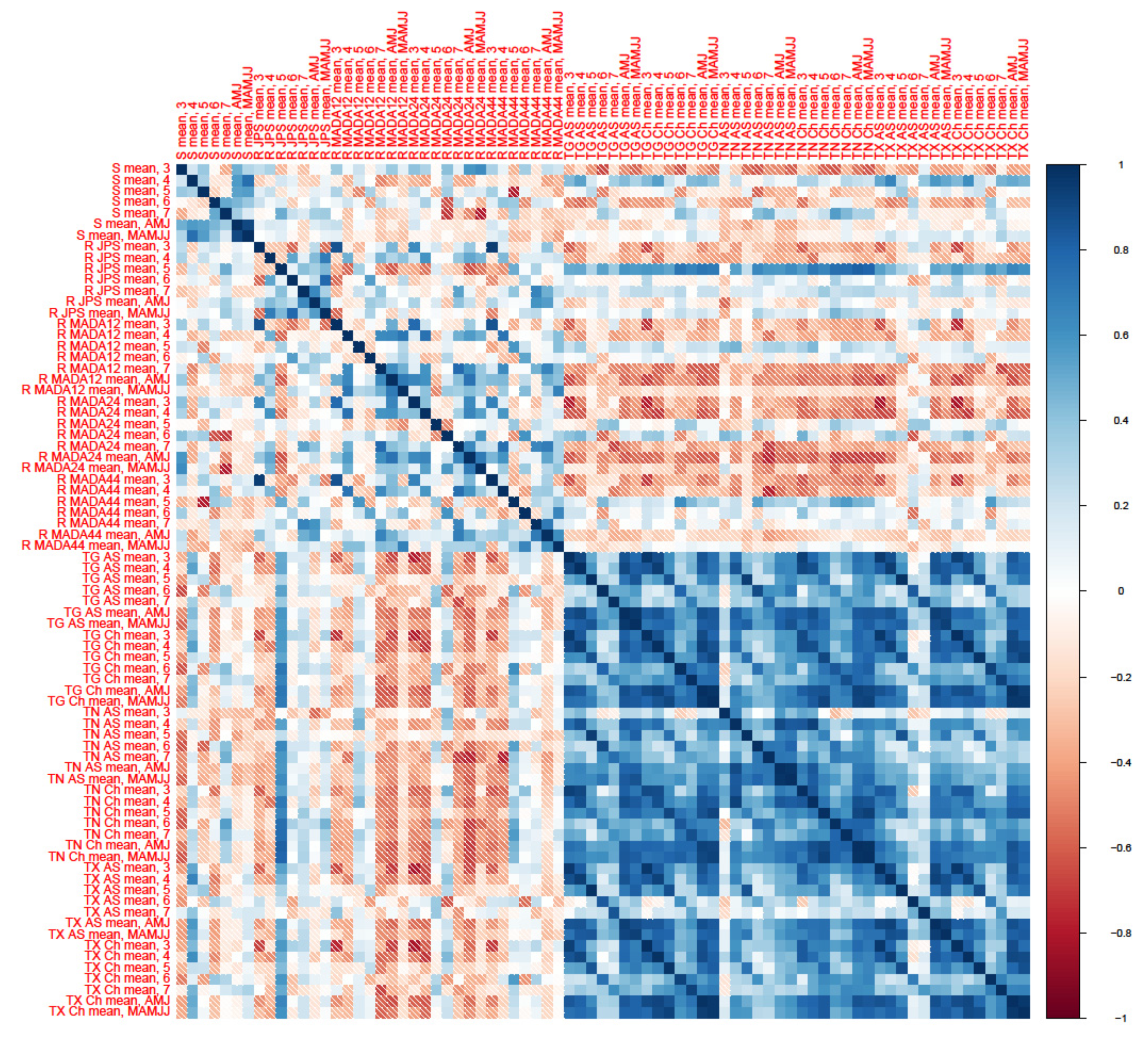
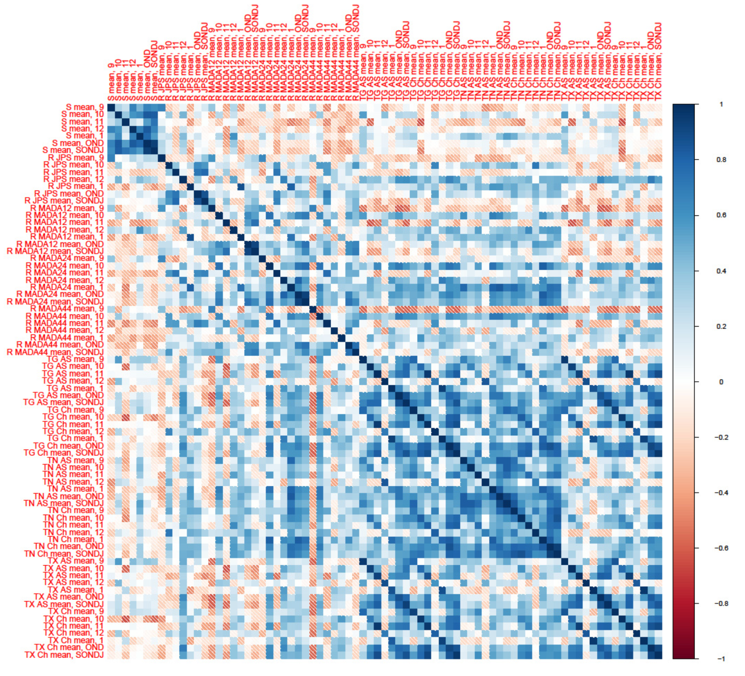
2.4. Correlation Analysis and Linear Regression

Further, correlation analysis was conducted on a seasonal scale, by associating the seasonal yields to the hydroclimatic variables for the relevant months. The Pearson correlation coefficient (r) was used to measure both the degree and direction (positive or negative) of the association.
Next, simple linear regression was conducted with monthly and seasonal rainfall, temperature, and streamflow indices as independent variables individually, and seasonal yield as the dependent variable. The coefficient of determination (R2) was used to evaluate and compare the variance in crop yield explained by the different indices. Regression analyses were conducted separately for the two separate cropping seasons as were the correlation analyses. The equations are as given in Table 3. All the regressed variables were first standardised based on the mean and standard deviation [46].
To complement the individual regressions and to explore any potential for improved predictive power based on multiple indices, multiple regression models were fitted based on the indices with absolute correlation values exceeding a threshold set at 0.65. A stepwise regression using both forward and backward selections was performed to find the best fit to the model based on the Akaike information criteria [47], and the best-fitted model considering all highly correlated indices for each season was produced. Additionally, the adjusted R2 was used to compare the multiple linear regression to the simple linear regression. This was to account for improvements to the R2 that was due to the addition of more independent variables, avoiding overfitting.
Finally, detection measures, i.e., probability of detection (POD) and false alarm rate (FAR) were computed, based on a standardised expected yield threshold of zero based on the mean of each season. In this specific analysis, standardised yield lower than zero was considered to yield below mean, resulting in a loss year. A confusion matrix was developed to account for the number of true and false positives and true and false negatives of the regression model prediction, whereby a positive was defined as a prediction or observation of yield below the expected. The equations of POD and FAR are as presented in Table 3.
All data processing and statistical analyses were conducted within the R computing environment.

3. Results

The results were organised as follows: first, the hydroclimatic indices were presented and their seasonal and intra-seasonal variabilities discussed. Then, the correlation and regression analysis were presented for season 1, followed by season 2. Next, a summative analysis using stepwise multiple regression was presented.

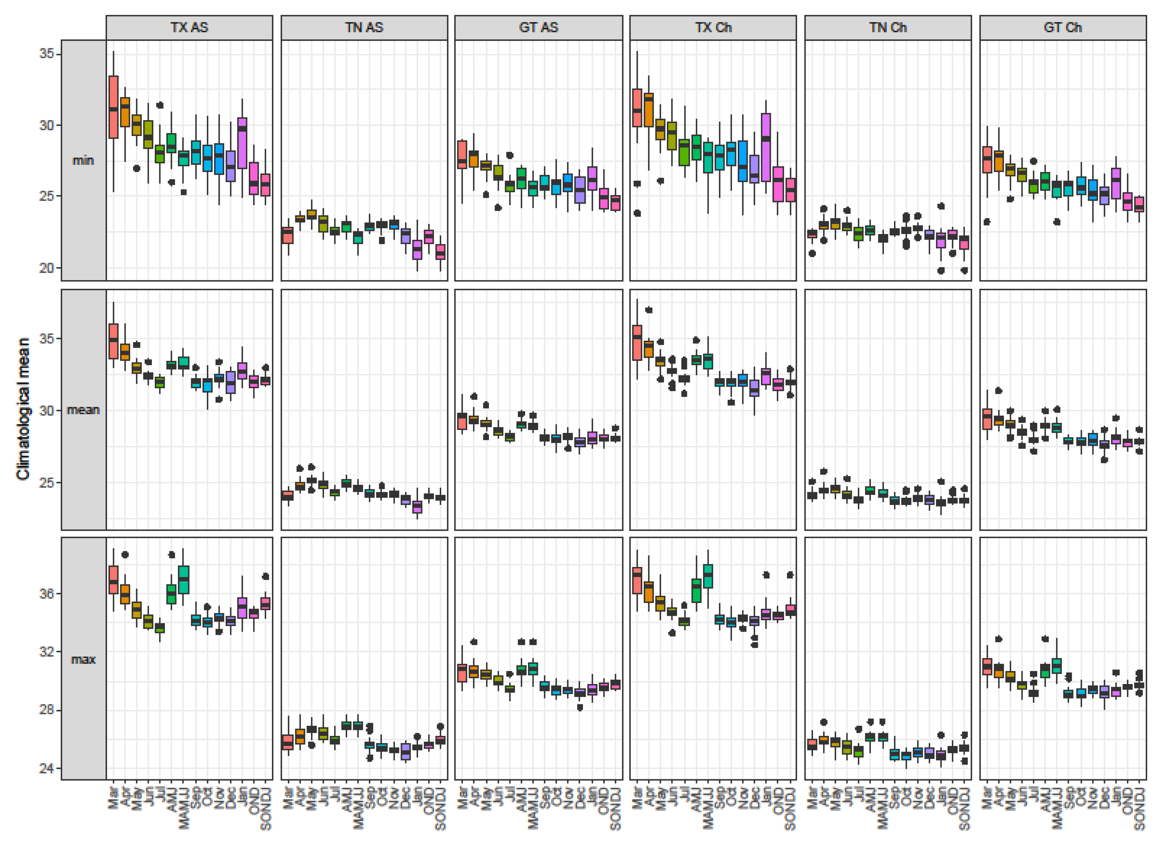
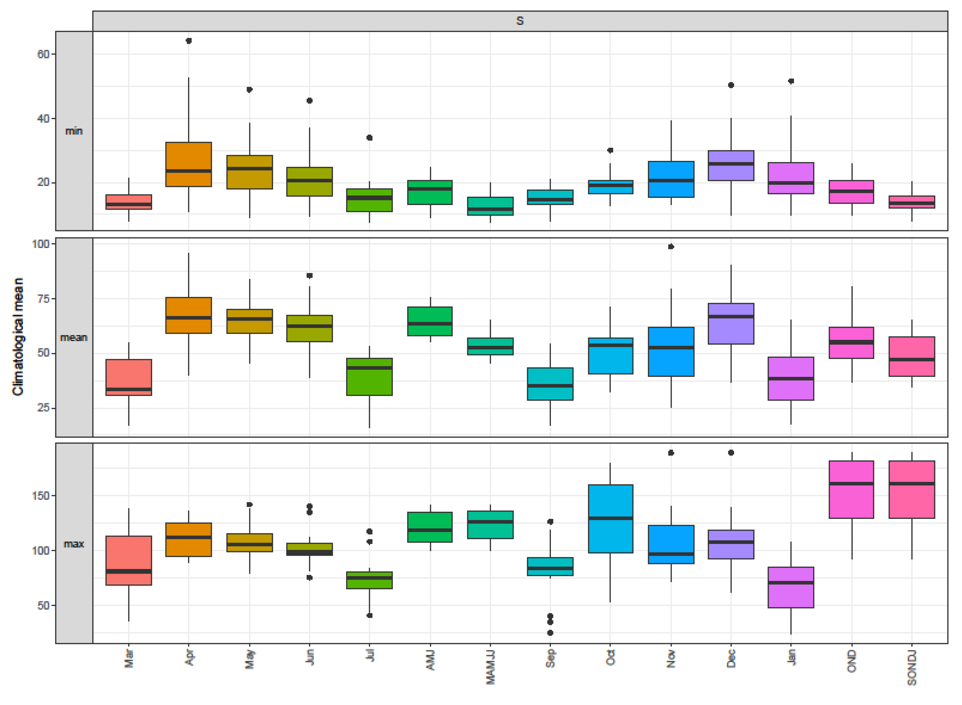
3.1. Seasonal and Intra-Seasonal Variability in the Hydroclimatic Indices

The climatological means of the mean indices indicated that the off-season or season 1 (March to July) had overall higher temperatures compared to the main season or season 2 (September to January) (Figure 2). In season 1, the highest maximum (TX) and average (GT) temperatures irrespective of the minimum, mean, or maximum indices were observed in March, declining towards the late season months of June and July. The lower temperatures remained throughout season 2, inflecting upwards only in January. On the other hand, the minimum temperature indices (TN) steadily inclined from March to May before declining towards the end of season 1 in July. Similarly, in season 2, TN indices inclined towards November before declining towards the end of season 2 in January. The variability observed at both stations Alor Setar (AS) and Chuping (Ch) was similar across all indices; nevertheless, TXmin values were noticeably higher in magnitude and range in Alor Setar compared to Chuping located further north.
The highest mean rainfall indices (Rmean) were observed in April in season 1 and October in season 2, while the lowest Rmean indices were observed in March and January of the respective seasons (Figure 3). The wet months corresponded to the inter-monsoon periods, whereas the dry months were coincident with the Northeast monsoon season. There was a spatial gradient whereby the lowest September to November rainfall means, and the strongest seasonality of the mean indices in season 1 (March to July) were observed in the northern-most station MADA12, in contrast to station MADA44 further south.
In terms of the extreme statistics, the maximum rainfall indices (Rmax) were highest in September (MADA12 and MADA44) and October (MADA24 and JPS) and lowest in January (all the four stations). The monthly variability aligned with that of the number of very wet days (D95p). On the other hand, the variability in wet days (DR1mm) and conversely the dry days (DD) corresponded to the variability of the mean rainfall indices. However, May was an exception in that the lower mean indices did not agree with the generally higher wet day indices compared to April and June. From these observations, it could be inferred that the May rainfall took the form of more days with lighter rain.
With streamflow, the minimum (Smin) and mean (Smean) indices were highest in December (season 2) and April (season 1) (Figure 4). In season 1, they remained high in May and June. With the exception of the April indices, these were uncharacteristic of the lower mean rainfall indices in the upstream catchment area (Rmean JPS) and could be explained via water demand management. Dam releases records (not shown) indicated the highest values in May and June, followed by the late season 2 months of December and January, and were in response to the irrigation requirement of the rice paddies. Thus, the streamflow indices of these months were largely attributable to the releases of water stored in the upstream reservoirs during the wetter months from September to November. By contrast, the maximum indices which were highest in April and October were directly related to the expected high flows during the inter-monsoon periods.
Between the mean indices, many were moderate to strongly correlated (Figure 5 and Figure 6) especially between the monthly and seasonal indices. In season 1, the strongest correlations were observed across temperature indices. With rainfall, temperature indices were noticeably positively correlated with Rmean at JPS Kuala Nerang, and to a lesser extent, Rmean at MADA12, MADA24, and MADA44 in May and June (up to July at MADA44). Otherwise, the correlation was predominantly negative in season 1. This is an effect of the monsoon, whereby temperature generally declines due to the shift from a dry late northeast monsoon in March into the inter-monsoon period and later to the southwest monsoon, which brings more rainfall. Between rainfall indices, there were noticeably weak positive correlations between Rmean at MADA12, MADA24, and MADA44 in selected months, but more apparent were the negative correlations between these station indices to Rmean at JPS in May.
Streamflow indices (Smean) in March were generally strongly positively correlated with Rmean across all stations and months. For the remaining months, there were no clear trends. However, there was the exception of the correlation with Rmean at JPS remaining generally positive, reflecting the proximity of the monitoring stations. Between the Smean of different months, cross-correlations were positive between the early season indices (March to May) but were negative between early (March to May) and late season (June and July) indices. This might be an effect of the higher amounts of reservoir releases in the mid-season (May-June) in years when the early season was abnormally drier.
In contrast, in Season 2, the cross-correlations between streamflow indices were more strongly positive and consistent throughout the wetter season. However, they were less negatively correlated with temperature and rainfall indices as compared to season 1. This again reflected a stronger reservoir regulation on the streamflow to compensate for the lesser amounts of rainfall in season 1 compared to season 2. Likewise, temperature indices were also positively cross-correlated as they were in season 1. However, the strength of the correlation diminished especially so with TXmean at both the Alor Setar and Chuping stations, reflecting the lower intra-seasonal variability of temperature in season 2. Furthermore, the temperature indices were also more positively correlated with rainfall indices, unlike in season 1, when they were more negatively correlated. This was an effect of the shifting from the inter-monsoon period (higher temperatures, higher rainfall) to the northeast monsoon (lower temperatures, lower rainfall) as the season progressed.

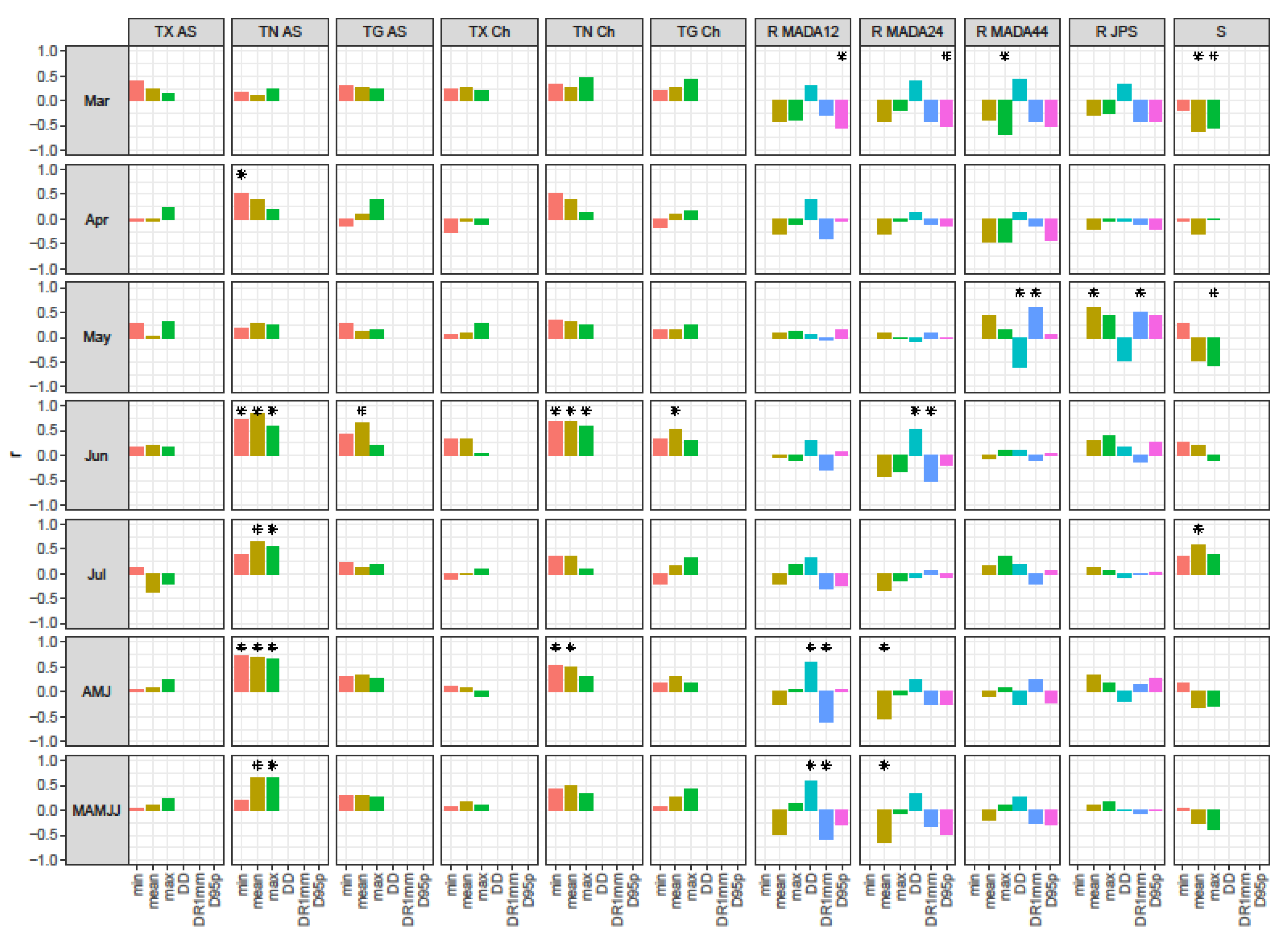
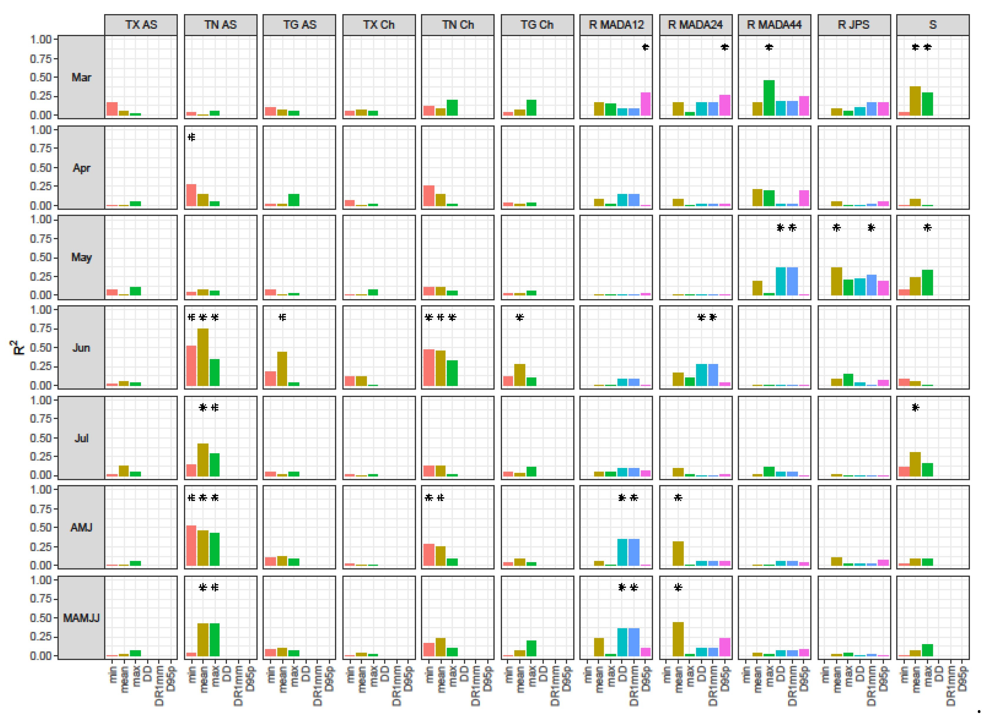
3.2. Hydroclimatic Controls on Yield in the Dry, Mainly Irrigated Season 1

In season 1 (Figure 7), regardless of indices, higher correlation values were observed in June and in the mid-growing season (AMJ). The strongest correlated indices were based on the mean and minimum temperature in both Alor Setar and Chuping stations: the highest positive correlation was +0.87 for the TNmean at Alor Setar in June and followed by TNmin and TNmean in both Alor Setar and Chuping in AMJ and June (r values between +0.67–+0.73). No significant negative correlation between yield and temperature was observed.
On the other hand, rainfall indices generally were negatively correlated with yield throughout the season, contradicting the temperature indices. The strongest negatively correlated indices were Pmax at MADA 44 in March (−0.67) and Pmean at MADA 24 of the full season (MAMJJ) (−0.66). Negative correlations were also found with the number of rain days (DR1mm) over the mid- (AMJ) and full-cropping season (MAMJJ) at MADA12 (r = −0.59), and to a lesser extent, at MADA24 in June (r = −0.52). This contrasted with the positive correlation with DR1mm in May at MADA44 (r = +0.60) and JPS (r = +0.51). Nevertheless, they aligned with correlations in the opposite direction observed with the DD indices. With the very wet days indices (D95p), correlations were generally negative, with significant correlations observed at MADA12 (r = −0.54) and MADA24 (r = −0.52). Positive but not significant correlations were found with D95p at JPS, which was in May-June in the upstream. This station also produced the highest positively correlated rainfall index in season 1 (dry season), i.e., with Rmean in May (r = +0.61).
Meanwhile, the correlations between streamflow and yield were predominantly negative in the early season but turned positive in the late season. A moderately strong negative correlation was found with Smean in March at −0.62, in contrast to a slightly weaker but positive correlation with Smean in July at +0.56.
When all indices and all months were considered, the yield was better correlated with the mean statistics than it was to the extreme statistics.
With the regression analysis, it was observed that March to May produced poorer results for temperature (Figure 8) but better regression with the rainfall and streamflow indices. The highest R2 value of 0.45 in the early season was obtained with a negatively correlated Rmax at MADA44 in March. Nevertheless, starting from June, temperature indices illustrated higher R2 values between 0.45–0.74, particularly for the minimum temperatures from Alor Setar and Chuping, indicating their abilities to explain 45–74% of the variance in the yield. The R2 remained relatively high until the end of the season. The regression values with the rainfall and streamflow indices declined during these months, not exceeding 0.40 despite their moderate correlations with yield.
The R2 with the rainfall indices furthermore showed some spatial contrasts: rainfall indices from stations located further north, i.e., MADA12 and MADA24 were poorer predictors of yield on the monthly basis, but this observation changed at the seasonal scale. In contrast, monthly indices from MADA44 and JPS were better predictors compared to their seasonal indices. This could be attributed to a higher interannual variability in the indices derived from MADA12 and MADA24, compared to that in MADA44 and JPS (refer to Figure 3). A poorer relationship with yields could therefore be related to the more unpredictable monthly indices in the two stations located further north. Meanwhile, streamflow indices were temporally inconsistent, indicating moderately good regression in alternative months, yet poor R2 from the season indices.
Overall, the results obtained from season 1 suggested that higher minimum temperatures during the late stage of growth especially at Alor Setar had the strongest, positive control on the dry season yield. This was followed by higher rainfall amounts at the start of the season that negatively impacted yield.

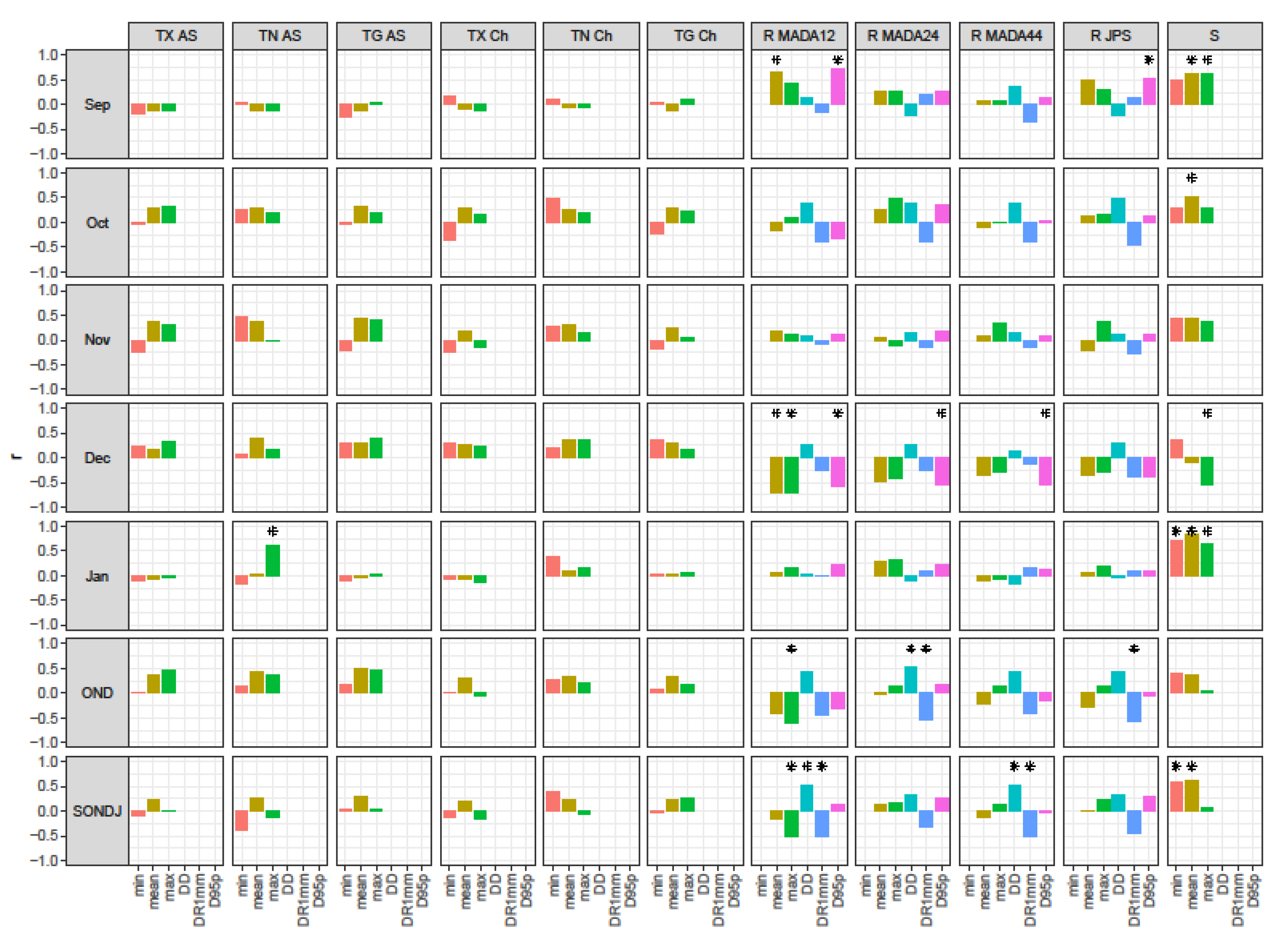
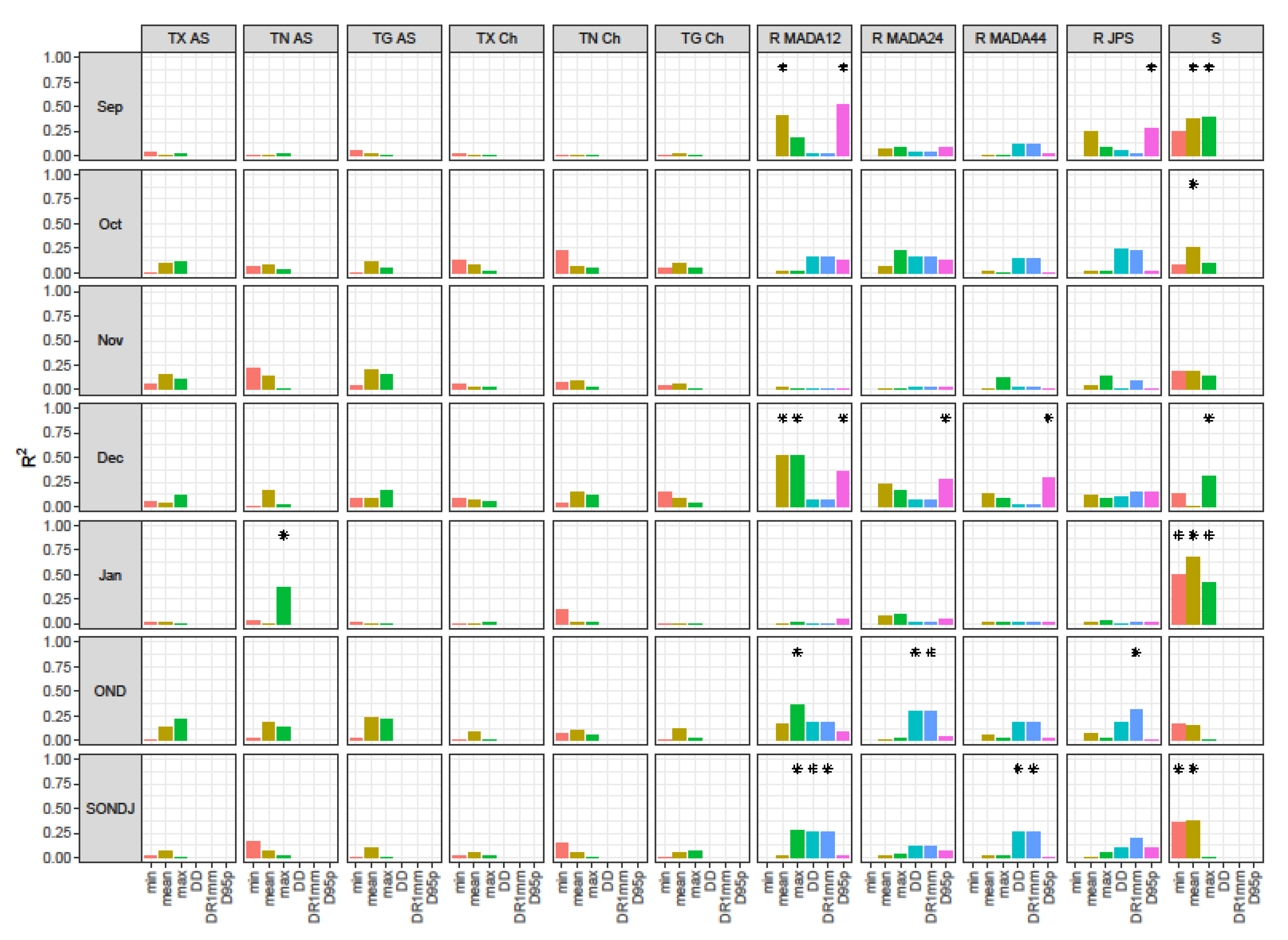
3.3. Hydroclimatic Controls on Yield in the Wetter Season 2

In season 2 (Figure 9), temperature indices continued to show correlations with yield, albeit weaker. However, the only significant correlation found with a temperature index was TNmax in January (r = +0.60).
On the other hand, with rainfall, September indices were strongly and positively correlated, while December indices were strongly but negatively correlated. The absolute correlation values were the highest in the northernmost station MADA12, declining as they move south (MADA24 and MADA44) and upstream (JPS) in the watershed. The highest positively correlated rainfall index was D95p in September at MADA12 (r = +0.72). Generally, positive correlations were observed with the very wet day indices between September and November, although they were only significant in September with MADA12 (r = +0.72) and JPS (r = +0.53). Meanwhile the highest negatively correlated monthly rainfall indices were Rmean and Rmax, also at MADA12 in December (r = −0.72). Negative correlations were also found with D95p in December for all MADA12, MADA24, and MADA44 stations (r from −0.53 to −0.59). Additional negative correlations were observed with the number of rain days (DR1mm) over the entire cropping season (SONDJ) at MADA12 and MADA44 (r = −0.51) and the mid-seasons (OND) in MADA24 and JPS (r = −0.54 and −0.56, respectively).
With streamflow, the strongest positive correlation was observed with Smean in January in season 2 (0.82). On the other hand, the strongest negative correlation was observed with Smax in December in season 2 (−0.56), corresponding to the rainfall indices at MADA12, MADA24, and MADA 44.
The highest correlation with yield for season 2 was +0.82 with Smean at Kuala Nerang in January. This was followed by D95p at MADA12 in September (r = +0.72) and Rmax and Rmean also at MADA12 in December (r = −0.72). The next strongest correlated indices were again positive with Smin and Smax in January (+0.65 and +0.71, respectively) and then Rmean (MADA12), Smax, and Smean in September (r = +0.62).
In translating these indices results into R2, values ranging between 0.38–0.67 were acquired (Figure 10), explaining up to two thirds of the variance in the yield. The best simple linear regressions were achieved with streamflow indices. A temporal trend was observed with the R2 values which were high in September but declined towards December, before increasing again in January. Further investigations of the climatological mean streamflow showed overall lower values in September and January than the rest of the season. This suggested that yield was more correlated and dependent on streamflow during the hydrologically drier parts of the season. In January, which showed the strongest correlation with yield, streamflow furthermore consisted of not only uncontrolled surface runoff but was also based on contribution from dam releases from the upstream reservoirs. This suggested that the explained variance in the yield was attributable to the dam releases.

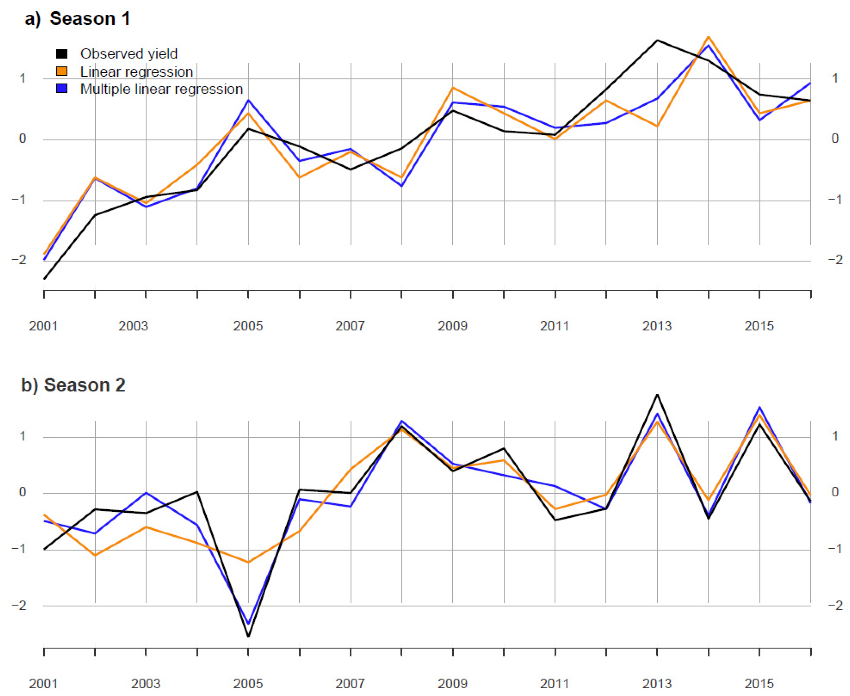
3.4. Stepwise Regression and Forecast Skill

The stepwise regression on multiple indices for both seasons (Table 4) illustrated a contradictory finding between the two cropping seasons. For season 1, the analysis only slightly increased the R2 from 0.74 to 0.75 (adjusted) by regressing against multiple indices, while in season 2, a more substantial R2 increase was observed from 0.67 to 0.84 (adjusted). Yield in season 1 was contrastingly a combination of high minimum temperatures in the late season and low mean seasonal rainfall, while yield in season 2 relied on higher streamflow in the late season (Smean in January) but lower mean rainfall in the preceding month (Rmean in December) and more very wet days in the early part of the season (D95p in September).
The resulting parsimonious models were furthermore evidence of high multicollinearity between different predictors. Particularly in season 1, the control on yield could mainly be explained via simple linear regression on TNmean Alor Setar (June), as evidenced by only a slight increase in the R2. The remaining unexplained variance might be attributable to other non-weather factors. Furthermore, the additional predictor variables in both seasons showed similarity in the timing of the influence, except for the odd D95p index in season 2.
A time-series comparison of the predicted versus the observed yields (Figure 11) revealed a closer agreement for the multiple linear regression compared to the simple linear regression, especially so for season 2. Nevertheless, the forecast statistics (Table 4) revealed otherwise for season 2. A loss in detection skill for loss years was observed with the multiple linear regression as indicated by lower POD and higher FAR compared to the remaining models. This was possibly due to the combination of independent regressors with indices and timing that was more mutually exclusive than those in season 1. The more distinct indices in season 2 would have a higher interannual variability and a lesser correlation with yield overall. Here, the lower volumetric error measured by the RMSE hence did not directly imply better skill with loss detection.

4. Discussion

In this section, we present a discussion of hydroclimatic controls in relation to various stages of crop growth and possible governing mechanisms. Next, these were contrasted between seasons and analysed with respect to the local climate.

4.1. Hydroclimatic Controls in Relation to Crop Phenological Stages

In this work, we found that correlation with yield was mostly positive and strongest with minimum temperature (TN) indices. In season 1, the positive correlations coincided with the rice growth stages of flowering and maturity, while in season 2, with the period of rice maturity and harvesting. As average temperatures in season 1 declined towards June and July in the Muda area, the abnormally low TNmean was likely to slow rice growth in the flowering and maturity stages. The flowering stage is the most sensitive stage and can lead to crop loss when it reduces below 25 °C [48]. Furthermore, in the maturity stage, a rise in temperature increases the rate of grain filling leading to a higher crop yield as long as the temperature remains below 35 °C [49]. A similar effect of low temperature was found in the index design for rice production in China [50]. However, the high-temperature damage found in the same study was not apparent in our case study (only weak negative correlation was present), possibly due to maximum temperatures rarely exceeding 35 °C outside of the vegetative period in season 1.
Meanwhile, positive correlations were found between yield and rainfall mean indices, as well as between yield and maximum indices in both season 1 and season 2. In season 1, they coincided with the late-stage vegetative rice growth stage (May) and reflected the critical crop water demand during this period, which was higher than in the other rice growth phases [40]. During the vegetative phase, water sufficiency increases the rate of tillering, whereas water stress causes the opposite effect [51,52]. The wet day indices in May were also positively correlated with yield in season 1 at MADA44 and JPS. By contrast, the wet day indices showed no positive correlation with yield in season 2. This was possibly due to the lower water demand and stress during the cooler, rainier season.
A positive correlation was observed between yield and streamflow throughout season 2 and in late season 1 (July). In both seasons, the strongest respective correlation occurred in the month associated with the maturity stage of the rice crop. Rice crops are dependent on water at field capacity during the entire growth phase. Hence, the strong correlation in the late season might have less to do with the stage of growth but was more reflective of the declining values in the streamflow during these months. This highlights the importance of reservoir releases to support the generally drier conditions of the end of the season and to sustain water in the rice paddy. In season 2, January Smean was also the strongest correlated with yield amongst all indices. Another possibility was that the higher than climatological average streamflow in January could be due to delayed planting and harvest and therefore delayed supplementary irrigation in some years. For other reasons related to temperature and rainfall variability that would be elaborated upon later, higher yields could have resulted.
More conspicuously, rainfall was negatively correlated with yield. The highest negatively correlated monthly rainfall mean and maximum indices coincided with the planting-to-vegetative phase (March, season 1) and the flowering-to-maturity phase (December, season 2). The negative impact of rainfall on yield in the early part of the season could stem from (1) disruption to land preparation activities and/or cultivation area loss [53] (2) reduction in sunlight due to cloud cover that could lower the rate of tillering [51,54]. On the other hand, its negative impact in the later growing periods could be attributed to the disruption of the flowering and pollination processes [55], as well as direct damage due to pluvial and fluvial flooding [24]. In the Muda area, historical reports have attributed losses to direct damage to rice crops because of flood inundation over long periods. Specifically, in the study area, fallen plants resulting from floods reduced the efficiency of harvesting by mechanized equipment.
In both seasons, negative correlations were also found with the number of rain days over the entire cropping season and, therefore, all stages of growth. The converse was true for dry days. These observations suggested that rainy days throughout the planting seasons might be detrimental to crop growth. It might be related to the concurrent reduction in solar radiation required for photosynthesizing new biomass. Moreover, rainfall is related to changes in environmental conditions such as increased nutrient leaching from topsoil and potentially limiting bio-uptake [56]. It also increases relative humidity, thus making the environment conducive to pests such as the brown planthopper [57,58], leaf folder [59], and white-backed planthopper [58,60].
The very wet day (D95p) statistics showed a contrasting trend of negative correlation with yield in March of season 1 but a robust positive correlation in September of season 2. Both seasons were related to the planting and vegetative growth stages. More very wet days would reduce yield in season 1, but by contrast, the same was expected to increase yield in season 2. A possible explanation for this was that these extreme events would disrupt land preparation and planting, causing a shift in the growing period for the season. While in season 1, this would result in a maturity phase and harvest in a period of lower temperatures (temperatures continuously decline from the onset of season 1); in season 2, this would result in more growth during periods of inclining temperatures (temperatures start to increase from December to January near the end of season 2) and in the same way, solar radiation. This mechanism only applied to very wet days in the early season, as negative correlations to D95p indices were observed again later in season 2. During this time, heavy rainfall days might be linked to losses by means of flooding damage.
To sum up, we hypothesize six primary mechanisms of hydroclimatic control on yield in the study area: firstly, at planting, more very wet days cause delay to planting—the effect on yield depends on the temperatures at the late season—which is positive if temperatures incline but negative if temperatures decline. Secondly, during the vegetative period, higher temperatures and sufficient rainfall but fewer very wet days improve tillering, thus increasing yield. Thirdly, during the maturity periods, water is less critical to growth compared to the vegetative and reproductive phase; on the contrary, excessive rainfall can disrupt reproductive processes and cause direct damage due to flooding. Fourthly, more frequent rainfall throughout the season may imply reduced solar radiation and nutrient availability to drive growth, as well as more likely destruction by pests. Fifthly, optimal temperatures are critical for growth throughout the season, and an abnormal decline would negatively impact yield. Lastly, irrigation water availability influences yield when direct rainfall is unable to fulfil the crop water demand.

4.2. Contrasting Hydroclimatic Controls on Yield between Dry and Wet Seasons

Our results illustrated a contrasting hydroclimatic influence on rice yields according to season. While temperature had stronger influences in the dry, irrigated season 1, streamflow had stronger influence in the wetter season 2. This might be explained by a stronger temperature variability in season 1 compared to season 2. Between the seasons, rainy days exhibited a stronger influence in the wet season compared to the dry season, as the lack of radiation due to cloud cover in season 1 for driving growth was possibly compensated by higher temperatures.
The contrasting controls were the result of climate drivers operating at larger scales. Specifically, the April inter-monsoon period and the southwest monsoon governed the weather variability in season 1, while the October inter-monsoon and northeast monsoon regulated season 2.
In season 1, the inter-monsoon at the beginning of the season was characterized by heavier convective rainfall, while the southwest monsoon beginning in May brought dry spells. This might explain the negative correlation of rainfall in the early season but a positive association in May. In season 1, although temperatures were higher and also more variable, rice farming was heavily supplemented by alternative water supply, and hence water availability did not present a limiting factor to crop growth despite higher evapotranspiration at higher temperatures. The optimized growth condition could explain the much higher yield in season 1, i.e., 5215 to 6595 MT ha−1 (median 6060 MT ha−1), than in season 2, i.e., 3936 to 6452 MT ha−1 (median 5386 MT ha−1). Additionally, the heavy rainfall during the inter-monsoon might have an adverse effect on the vegetative growth due to the lack of solar radiation and flooded conditions. Only during the drier period of the southwest monsoon that rainfall started to show positive impacts.
On the other hand, in season 2, i.e., the wet season overlapped with the inter-monsoon in October and the beginning of the northeast monsoon starting in November. During this inter-monsoon period and the northeast monsoon, the temperature was consistently lower throughout the season except in the late season and with higher but more variable rainfall patterns, resulting in an overall lower yield compared to season 1. Under this environmental condition, however, rice growth seemed to embrace the lower temperatures, and water availability became more limiting. These weather conditions explained the insignificant correlations of temperature throughout the season. Instead, positive correlations to rainfall in September was associated with relatively higher average rainfall, whereas negative correlations to rainfall in December occurred as the average rainfall started to lessen as the Northeast monsoon strengthened. Due to the lower temperatures of this season, too much rainfall was detrimental to crop growth and especially during the drier period later in the season. It was possible that during this time crop growth was trying to compensate for the lack of radiation during the wetter early part of the season, and an uncharacteristically wet late season (December) would hamper its progress. This view was strengthened by the observation that both (1) higher streamflow as a result of higher reservoir releases in January, and (2) higher rainfall in September were positively correlated with yield. A backward shift to the growing season was inferred from the early season wet condition and the very late season irrigation, benefiting from a maturity stage that extended into the period when the season became drier and temperatures started to increase.
Our findings with rainfall effects on yield generally agreed with the findings on rice cultivation in Thailand [61]; however, a positive effect instead of a negative effect of temperature was found in our work. This is reasonable as even hydroclimatic controls on yield can vary even within countries ([62], and references therein). Furthermore, it may be that local temperatures are optimal for our local rice varieties. Our findings are, moreover, in line with previous findings of the negative control of mean rainfall and positive control of mean temperature in Malaysia at the annual scale [63,64]. Lastly, while drought specific indices have explained yield variabilities in drought-prone areas [62], in our work, this effect is confounded by irrigation management. Correlations between yield and rainfall have been observed to weaken where irrigation is a major contributor to crop water demand [61]. Nevertheless, our analysis has shown that this is very context specific, whereby the overall climatology and inter- and intra-seasonal variabilities of various hydroclimatic parameters relevant for growth, and their derivative indices, need to be considered more systematically and holistically.

5. Conclusions

A prior coarser-scale study linking yield to rainfall and temperature indices for different planting zones across Malaysia identified suitable indices for two out of the five zones investigated and had called for a more robust indices selection considering more weather parameters [65]. In our study, the relationships between intra-annual hydroclimatic variability and rice yield were explored systematically in the Muda area. The results indicated that different monthly statistics based on daily minimum and maximum temperatures, rainfall, and streamflow were correlated with rice yields at different growing stages at different seasons. Sunlight, temperature, and water are all drivers of plant growth, and there exists a trade-off between water supply from direct rainfall, and temperature and solar radiation throughout the planting seasons. As a result, the timing (in relation to crop stages) and magnitude of the hydroclimatic indices critically influence overall crop growth.
This study furthermore provides evidence that a consideration of multiple individual and combined hydroclimatic indices is essential in the construction of index-based insurance schemes in areas with multi-season cropping being practised. While minimum temperature is the dominant index for the drier season (season 1), it is streamflow proxying for late-season reservoir releases for the wetter season (season 2), enhanced by rainfall. This may run counter to possible preconceptions of seasonal influence on the yield; for example, sufficient reservoir supply may be perceived to influence yield more in the dry season compared to the wet season due to hydrological drought [24]. Here, the divergence in the dry season may likely be due to adequate water demand management, in which there is a high degree of built-in redundancy based on multiple irrigation water resources which are centrally managed at the watershed scale. On the other hand, in the wet season, the reason for the anomaly is that the water supply from the reservoir is still being depended upon during the late stage of the wet season as rainfall and streamflow start to decline.
While hydroclimatic variability is beyond human control, reservoir releases to sustain irrigation can form future operational strategies to mitigate the risk of yield losses. More specifically, for developing weather index policy for the area, contracts based on monthly minimum statistics of the minimum-temperature (e.g., [60]) and water-supply-based indices (e.g., [22,23]) need to be paid attention to in addition to the more established use of rainfall indices. Furthermore, the predictive power of the regression models substantially varies between the dry and wet cropping seasons, and by the type of indices used in the regression, but consideration of more than one predictor could improve the wet season yield estimation. These compounded effects have not been well studied in the weather index literature, which may be due to the difficulty of developing an indemnity structure with more than one trigger.
Furthermore, the study illustrates the importance of considering the time aspect of the indices as they relate to different phenological phases of plants in minimising basis risk. Our findings clearly indicate that the indices influencing seasonal yield in the area are well defined in time; hence, temporal basis risk in any insurance instrument based on these indices can be adequately addressed by zooming into very specific time windows. Lastly, understanding the processes underlying the results of correlation and regression as they relate to crop phenological stages could help improve the transparency of weather index construction and its acceptability by farmers and insurance providers. This is important, as evidenced by poor uptake of the index insurance due to a lack of understanding of the design in many different studies (e.g., [66,67,68]).
This study was limited to the understanding of the role of hydroclimatic indices. The variability that was caused by other factors such as pests, nutrient management, and planting dates could not be construed due to the sole reliance on the time series of hydroclimatic parameters and crop yield. Furthermore, this study looked at the entire agricultural production scale from a meso-/basin-scale lens, due to the data availability, and did not attempt to formally address the third component of basis risk, i.e., spatial basis risk [69], despite systematically addressing design and temporal basis risk. The study also did not attempt to propose a contract design based on actuarial analysis. Future work can improve on this study by looking at more refined scales, for example by analysing the yield against hydroclimatic variability at smaller administrative scales.

Author Contributions

Z.Z. and N.R. prepared the concept. N.R. performed the data collection and processing. Z.Z. and A.J. performed the regression analysis. Z.Z., F.M.M., and A.J. interpreted the results and wrote the manuscript. M.J.A., N.R., A.J., B.M.R. and K.N. validated the result and edited the manuscript. All authors have read and agreed to the published version of the manuscript.

Funding

The research was funded by the Ministry of Higher Education via the Fundamental Research Grant Scheme FRGS/1/2017/WAB05/UPM/02/3.

Institutional Review Board Statement

Not applicable.

Informed Consent Statement

Not applicable.

Data Availability Statement

The data used in this study are subjected to the data provider’s data licensing restrictions and may be furnished upon request to the corresponding author.

Acknowledgments

The authors would like to thank MADA for providing the necessary data for undertaking this research. The authors also thank the Department of Irrigation and Drainage, Malaysia (DID) for free use of the rainfall station data.

Conflicts of Interest

The authors declare no conflict of interest.

References

  1. Prasad, R.; Shivay, Y.S.; Kumar, D. Current status, challenges, and opportunities in rice production. In Rice Production Worldwide; Springer: Berlin/Heidelberg, Germany, 2017; pp. 1–32. [Google Scholar]
  2. Siwar, C.; Idris, N.D.M.; Yasar, M.; Morshed, G. Issues and challenges facing rice production and food security in the granary areas in the East Coast Economic Region (ECER), Malaysia. Res. J. Appl. Sci. Eng. Technol. 2014, 7, 711–722. [Google Scholar] [CrossRef]
  3. Bishwajit, G.; Sarker, S.; Kpoghomou, M.-A.; Gao, H.; Jun, L.; Yin, D.; Ghosh, S. Self-sufficiency in rice and food security: A South Asian perspective. Agric. Food Secur. 2013, 2, 10. [Google Scholar] [CrossRef] [Green Version]
  4. Omar, S.C.; Shaharudin, A.; Tumin, S.A. The Status of the Paddy and Rice Industry in Malaysia; Khazanah Research Institute: Kuala Lumpur, Malaysia, 2019. [Google Scholar]
  5. Faostat. FAO Statistical Pocketbook 2015 World Food and Agriculture 2015; FAO: Rome, Italy, 2015. [Google Scholar]
  6. Vaghefi, N.; Shamsudin, M.N.; Radam, A.; Rahim, K.A. Impact of climate change on food security in Malaysia: Economic and policy adjustments for rice industry. J. Integr. Environ. Sci. 2016, 13, 19–35. [Google Scholar] [CrossRef]
  7. Alam, M.; Siwar, C.; Islam, R.; Toriman, M.E.; Basri, T. Climate change and vulnerability of paddy cultivation in north-west Selangor, Malaysia: A survey of farmers’ assessment/Md. Mahmudul Alam…[et al.]. Acad. Ser. Univ. Teknol. MARA Kedah 2011, 6, 45–56. [Google Scholar]
  8. Pio Lopez, G. ‘Economic reforms for paddy sub-sector’. Star Online. 2007, 25. Available online: https://www.thestar.com.my/business/business-news/2007/06/25/economic-reforms-for-paddy-subsector (accessed on 13 January 2021).
  9. Asia Pacific Adaptation Network. Promoting Risk Financing in the Asia Pacific Region: Lessons from Agriculture Insurance in Malaysia, Philippines and Vietnam; Institute for Global Environmental Strategies (IGES): Kanagawa, Japan, 2013. [Google Scholar]
  10. Mahul, O.; Stutley, C.J. Government Support to Agricultural Insurance: Challenges and Options for Developing Countries; World Bank: Washington, DC, USA, 2010. [Google Scholar]
  11. Porth, L.; Lin, J.; Boyd, M.; Pai, J.; Zhang, Q.; Wang, K. Factors affecting farmers’ willingness to purchase weather index insurance in the Hainan Province of China. Agric. Financ. Rev. 2015, 75, 103–113. [Google Scholar]
  12. Choudhury, A.; Jones, J.; Okine, A.; Choudhury, R. Drought-triggered index insurance using cluster analysis of rainfall affected by climate change. J. Insur. Issues 2016, 39, 169–186. [Google Scholar]
  13. Khalil, A.F.; Kwon, H.; Lall, U.; Miranda, M.J.; Skees, J. El Niño–Southern Oscillation–based index insurance for floods: Statistical risk analyses and application to Peru. Water Resour. Res. 2007, 43. [Google Scholar] [CrossRef]
  14. Barnett, B.J.; Mahul, O. Weather index insurance for agriculture and rural areas in lower-income countries. American J. Agric. Econ. 2007, 89, 1241–1247. [Google Scholar] [CrossRef]
  15. Barrett, C.B.; Barnett, B.J.; Carter, M.R.; Chantarat, S.; Hansen, J.W.; Mude, A.G.; Osgood, D.; Skees, J.R.; Turvey, C.G.; Ward, M.N. Poverty Traps and Climate Risk: Limitations and Opportunities of Index-Based Risk Financing. Iri Tech. Rep. No. 07-02. 2007. Available online: https://iri.columbia.edu/ (accessed on 13 January 2021).
  16. Cao, M.; Li, A.; Wei, J.Z. Precipitation modeling and contract valuation: A frontier in weather derivatives. J. Altern. Invest. 2004, 7, 93–99. [Google Scholar] [CrossRef]
  17. Chen, W.; Hohl, R.; Tiong, L.K. Rainfall index insurance for corn farmers in Shandong based on high-resolution weather and yield data. Agric. Financ. Rev. 2017, 77, 337–354. [Google Scholar] [CrossRef]
  18. Heimfarth, L.E.; Musshoff, O. Weather index-based insurances for farmers in the North China Plain: An analysis of risk reduction potential and basis risk. Agric. Financ. Rev. 2011, 71, 218–239. [Google Scholar] [CrossRef]
  19. Breustedt, G.; Bokusheva, R.; Heidelbach, O. Evaluating the potential of index insurance schemes to reduce crop yield risk in an arid region. J. Agric. Econ. 2008, 59, 312–328. [Google Scholar] [CrossRef]
  20. Pelka, N.; Musshoff, O. Hedging effectiveness of weather derivatives in arable farming–is there a need for mixed indices? Agric. Financ. Rev. 2013, 73, 358–372. [Google Scholar] [CrossRef]
  21. Vedenov, D.V.; Barnett, B.J. Efficiency of weather derivatives as primary crop insurance instruments. J. Agric. Resour. Econ. 2004, 29, 387–403. [Google Scholar]
  22. Brown, C.; Carriquiry, M. Managing hydroclimatological risk to water supply with option contracts and reservoir index insurance. Water Resour. Res. 2007, 43. [Google Scholar] [CrossRef]
  23. Leiva, A.J.; Skees, J.R. Using Irrigation Insurance to Improve Water Usage of the Rio Mayo Irrigation System in Northwestern Mexico. World Dev. 2008, 36, 2663–2678. [Google Scholar] [CrossRef]
  24. Siebert, A. Analysis of index insurance potential for adaptation to hydroclimatic risks in the west African Sahel. WeatherClim. Soc. 2016, 8, 265–283. [Google Scholar] [CrossRef]
  25. Kost, A.; Läderach, P.; Fisher, M.; Cook, S.; Gómez, L. Improving index-based drought insurance in varying topography: Evaluating basis risk based on perceptions of Nicaraguan hillside farmers. PLoS ONE 2012, 7, e51412. [Google Scholar] [CrossRef] [PubMed] [Green Version]
  26. Stojanovski, P.; Dong, W.; Wang, M.; Ye, T.; Li, S.; Mortgat, C.P. Agricultural risk modeling challenges in China: Probabilistic modeling of rice losses in Hunan Province. Int. J. Disaster Risk Sci. 2015, 6, 335–346. [Google Scholar] [CrossRef] [Green Version]
  27. Carter, M.; De Janvry, A.; Sadoulet, E.; Sarris, A. Index Insurance for Developing Country Agriculture: A reassessment. Annu. Rev. Resour. Econ. 2017, 9, 421–438. [Google Scholar] [CrossRef]
  28. Leblois, A.; Quirion, P. Agricultural insurances based on meteorological indices: Realisations, methods and research challenges. Meteorol. Appl. 2013, 20, 1–9. [Google Scholar] [CrossRef] [Green Version]
  29. Kang, Y.; Khan, S.; Ma, X. Climate change impacts on crop yield, crop water productivity and food security–A review. Prog. Nat. Sci. 2009, 19, 1665–1674. [Google Scholar] [CrossRef]
  30. Lal, R.; Uphoff, N.; Stewart, B.A.; Hansen, D.O. Climate Change and Global Food Security; CRC Press: Boca Raton, FL, USA, 2005. [Google Scholar]
  31. Magadza, C.H.D. Climate change impacts and human settlements in Africa: Prospects for adaptation. Environ. Monit. Assess. 2000, 61, 193–205. [Google Scholar] [CrossRef]
  32. Austin, O.C.; Baharuddin, A.H. Risk in Malaysian agriculture: The need for a strategic approach and a policy refocus. Kajian Malaysia J. Malays. Stud. 2012, 30, 21–50. [Google Scholar]
  33. Prabhakar, S.; Suryahadi, S.; Setyanto, P. Mitigation co-benefits of adaptation actions in agriculture: An opportunity for promoting climate smart agriculture in Indonesia. Asian J. Environ. Disaster Manag. 2013, 5, 261–276. [Google Scholar] [CrossRef]
  34. Academy of Science Malaysia. El Niño: A Review of Scientific Understanding and the Impact of 1997/98 Event in Malaysia; Academy of Science Malaysia: Kuala Lumpur, Malaysia, 2018. [Google Scholar]
  35. Al-Amin, A.Q.; Alam, G.M. Impact of El-Niño on agro-economics in Malaysia and the surrounding regions: An analysis of the events from 1997–1998. Asian J. Earth Sci. 2016, 9, 1–8. [Google Scholar]
  36. Hanafiah, M.M.; Ghazali, N.F.; Harun, S.N.; Abdulaali, H.; Abdul-Hasan, M.J.; Kamarudin, M.K.A. Assessing water scarcity in Malaysia: A case study of rice production. Desalin. Water Treat 2019, 149, 274–287. [Google Scholar] [CrossRef] [Green Version]
  37. Maidin, K.H.; Mohamad, C.K.B.I.; Othman, S.K.B. Impacts of natural disasters on the paddy production and its implications to the economy. Fftc Agric. Policy Platf. 2015. Available online: https://ap.fftc.org.tw/article/970 (accessed on 13 January 2021).
  38. Firdaus, R.B.R.; Leong Tan, M.; Rahmat, S.R.; Senevi Gunaratne, M. Paddy, rice and food security in Malaysia: A review of climate change impacts. Cogent Soc. Sci. 2020, 6, 1818373. [Google Scholar] [CrossRef]
  39. Department of Statistics Malaysia. Press Release: Demographic Statistics First Quarter 2020, Malaysia 2020; Department of Statistics: Putrajaya, Malaysia, 2020.
  40. Lansigan, F.P. Implementation Issues in Weather Index-based Insurance for Agricultural Production: A Philippine Case Study; IGES: Hayama, Japan; SEARCA: Los Baños, Laguna, Philippines, 2015; Available online: https://www.searca.org/pubs/briefs-notes?pid=288 (accessed on 13 January 2021).
  41. Suhaila, J.; Deni, S.M.; Zin, W.Z.W.; Jemain, A.A. Trends in peninsular Malaysia rainfall data during the southwest monsoon and northeast monsoon seasons: 1975–2004. Sains Malays. 2010, 39, 533–542. [Google Scholar]
  42. Wong, C.L.; Liew, J.; Yusop, Z.; Ismail, T.; Venneker, R.; Uhlenbrook, S. Rainfall characteristics and regionalization in Peninsular Malaysia based on a high resolution gridded data set. Water 2016, 8, 500. [Google Scholar] [CrossRef] [Green Version]
  43. Julien, P.Y.; Ghani, A.A.; Zakaria, N.A.; Abdullah, R.; Chang, C.K. Case study: Flood mitigation of the Muda River, Malaysia. J. Hydraul. Eng. 2010, 136, 251–261. [Google Scholar] [CrossRef] [Green Version]
  44. Aisyah Baharudin, S.; Arshad, F.M.; Baharudin, S.A. Water management in the paddy area in MADA. Econ. Technol. Manag. Rev. 2015, 10, 21–29. Available online: http://etmr.mardi.gov.my/Content/ETMRVol.10a(2015)/Vol10a(3).pdf (accessed on 13 January 2021).
  45. Peña-Angulo, D.; Reig-Gracia, F.; Domínguez-Castro, F.; Revuelto, J.; Aguilar, E.; van der Schrier, G.; Vicente-Serrano, S.M. ECTACI: European Climatology and Trend Atlas of Climate Indices (1979–2017). J. Geophys. Res. Atmos. 2020, 125, e2020JD032798. [Google Scholar] [CrossRef]
  46. Bring, J. How to standardize regression coefficients. Am. Stat. 1994, 48, 209–213. [Google Scholar]
  47. Cavanaugh, J.E. Unifying the derivations for the Akaike and corrected Akaike information criteria. Stat. Probab. Lett. 1997, 33, 201–208. [Google Scholar] [CrossRef]
  48. Ghadirnezhad, R.; Fallah, A. Temperature effect on yield and yield components of different rice cultivars in flowering stage. Int. J. Agron. 2014, 846707. [Google Scholar] [CrossRef]
  49. Krishnan, P.; Ramakrishnan, B.; Reddy, K.R.; Reddy, V.R. High-temperature effects on rice growth, yield, and grain quality. Adv. Agron. 2011, 111, 87–206. [Google Scholar]
  50. Guo, J.; Jin, J.; Tang, Y.; Wu, X. Design of temperature insurance index and risk zonation for single-season rice in response to high-temperature and low-temperature damage: A case study of Jiangsu province, China. Int. J. Environ. Res. Public Health 2019, 16, 1187. [Google Scholar] [CrossRef] [Green Version]
  51. Abbas, S.; Mayo, Z.A. Impact of temperature and rainfall on rice production in Punjab, Pakistan. Environ. Dev. Sustain. 2021, 23, 1706–1728. [Google Scholar] [CrossRef]
  52. Joseph, K.; Menon, P.K.G.; Koruth, A. Influence of weather parameters on wetland rice yields in Kerala. Oryza 1988, 25, 365–368. [Google Scholar]
  53. Asada, H.; Matsumoto, J. Effects of rainfall variation on rice production in the Ganges-Brahmaputra Basin. Clim. Res. 2009, 38, 249–260. [Google Scholar] [CrossRef] [Green Version]
  54. Sridevi, V.; Chellamuthu, V. Impact of weather on rice–A review. Int. J. Appl. Res. 2015, 1, 825–831. [Google Scholar]
  55. Lawson, D.A.; Rands, S.A. The effects of rainfall on plant–pollinator interactions. Arthropod-Plant Interact. 2019, 13, 561–569. [Google Scholar] [CrossRef] [Green Version]
  56. Mo’allim, A.A.; Kamal, M.R.; Muhammed, H.H.; Mohd Soom, M.A.; Zawawi, M.; Wayayok, A.; Bt, H. Assessment of nutrient leaching in flooded paddy rice field experiment using Hydrus-1D. Water 2018, 10, 785. [Google Scholar] [CrossRef] [Green Version]
  57. Sawada, H.; Kusmayadi, A.; Gaib Subroto, S.W.; Suwardiwijaya, E. Comparative analysis of population characteristics of the brown planthopper, Nilaparvata lugens Stål, between wet and dry rice cropping seasons in West Java, Indonesia. Popul. Ecol. 1993, 35, 113–137. [Google Scholar] [CrossRef]
  58. Madhuri, G.; Dash, P.C.; Rout, K.K. Effect of weather parameters on population dynamics of paddy pests. Int. J. Curr. Microbiol. Appl. Sci. 2017, 6, 2049–2053. [Google Scholar] [CrossRef]
  59. Rath, P.C.; Jena, M.; Behera, K.S.; Sasmal, S. Pest outbreaks and resurgence in rice ecosystem in Odisha—A retrospect. In Proceedings of the 7th National Seminar on Emerging Climate Change Issues and Sustainable Management Strategies, Bhubaneswar, India, 8–19 February 2014; pp. 20–21. [Google Scholar]
  60. Gubbaiah, D.D.; Revana, H.P. The rice white-backed plant hopper (WBPH) in Karnataka. Int. Rice Res. Newsl. 1987, 12, 34. [Google Scholar]
  61. Prabnakorn, S.; Maskey, S.; Suryadi, F.X.; de Fraiture, C. Rice yield in response to climate trends and drought index in the Mun River Basin, Thailand. Sci. Total Environ. 2018, 621, 108–119. [Google Scholar] [CrossRef]
  62. Kattelus, M.; Salmivaara, A.; Mellin, I.; Varis, O.; Kummu, M. An evaluation of the Standardized Precipitation Index for assessing inter-annual rice yield variability in the Ganges–Brahmaputra–Meghna region. Int. J. Climatol. 2016, 36, 2210–2222. [Google Scholar] [CrossRef]
  63. Kaffashi, S. Assessing the impacts of climate change on paddy production in Malaysia. Res. J. Environ. Sci. 2014, 8, 331–341. [Google Scholar]
  64. Firdaus, R.R.; Latiff, I.A.; Borkotoky, P. The impact of climate change towards Malaysian paddy farmers. J. Dev. Agric. Econ. 2012, 5, 57–66. [Google Scholar] [CrossRef] [Green Version]
  65. Wen, Y.W.J.; Ponnusamy, R.R.; Kang, H.M. Application of weather index-based insurance for paddy yield: The case of Malaysia. Int. J. Adv. Appl. Sci. 2019, 6, 51–59. [Google Scholar]
  66. Adegoke, J.; Pramod, A.; Rüegg, M.; Hansen, J.; Cuellar, D.; Diro, R.; Shaw, R.; Hellin, J.; Greatrex, H.; Zougmoré, R. Review of Index-Based Insurance for Climate-Smart Agriculture: Improving Climate Risk Transfer and Management for Climate-Smart Agriculture—A Review of Existing Examples of Successful Index-Based Insurance for Scaling up; Food Agriculture Organization (FAO): Rome, Italy, 2017. [Google Scholar]
  67. Kumar, D.S.; Barah, B.C.; Ranganathan, C.R.; Venkatram, R.; Gurunathan, S.; Thirumoorthy, S. An analysis of farmers’ perception and awareness towards crop insurance as a tool for risk management in Tamil Nadu. Agric. Econ. Res. Rev. 2011, 24, 37–46. [Google Scholar]
  68. Rathod, M.K.; Chavan, S.U.; Rathod, T. Farmers Awareness and Perception towards Crop Insurance as a Risk Management Tool. J. Glob. Commun. 2016, 9, 118–122. [Google Scholar] [CrossRef]
  69. Dalhaus, T.; Finger, R. Can gridded precipitation data and phenological observations reduce basis risk of weather index–based insurance? WeatherClim. Soc. 2016, 8, 409–419. [Google Scholar] [CrossRef]
Figure 1. Study area with elevation and location of temperature, rainfall, and streamflow monitoring stations. The rice cultivation areas are divided into four regions, which are demarked by orange boundary lines.
Sustainability 13 05207 g001
Figure 2. Distribution of climatological means for the monthly and seasonal temperature indices based on 16 years of data (one sample per year). MAMJJ stands for Mar-Apr-May-Jun-July which is season 1 (off-season), while AMJ indicates Apr-May-Jun, which are the mid-season months. Likewise, SONDJ stands for Sep-Oct-Nov-Dec-Jan, which is season 2 (main season), while OND indicates Oct-Nov-Dec which are the mid-season months.
Sustainability 13 05207 g002
Figure 3. Distribution of climatological means for the monthly and seasonal rainfall indices based on 16 years of data (one sample per year). MAMJJ stands for Mar-Apr-May-Jun-July which is season 1 (off-season), while AMJ indicates Apr-May-Jun, which are the mid-season months. Likewise, SONDJ stands for Sep-Oct-Nov-Dec-Jan, which is season 2 (main season), while OND indicates Oct-Nov-Dec which are the mid-season months.
Sustainability 13 05207 g003
Figure 4. Distribution of climatological means for the monthly and seasonal streamflow indices based on 16 years of data (one sample per year). MAMJJ stands for Mar-Apr-May-Jun-July which is season 1 (off-season), while AMJ indicates Apr-May-Jun, which are the mid-season months. Likewise, SONDJ stands for Sep-Oct-Nov-Dec-Jan, which is season 2 (main season), while OND indicates Oct-Nov-Dec which are the mid-season months.
Sustainability 13 05207 g004
Figure 5. Correlation between the monthly and seasonal hydroclimatic mean indices for season 1. Here, 3–7 indicate the months of March, April, May, June, and July. MAMJJ stands for Mar-Apr-May-Jun-July which is season 1 (off-season), while AMJ indicates Apr-May-Jun, which are the mid-season months.
Sustainability 13 05207 g005
Figure 6. Correlation between the monthly and seasonal hydroclimatic mean indices for season 2. Here, 9–12 and 1 indicate the months from September to December and January. SONDJ stands for Sep-Oct-Nov-Dec-Jan, which is season 2 (main season), while OND indicates Oct-Nov-Dec which are the mid-season months.
Sustainability 13 05207 g006
Figure 7. Correlation between yield and monthly and seasonal hydroclimatic indices for season 1. Statistically significant correlation at p = 0.05 is demarked by *.
Sustainability 13 05207 g007
Figure 8. Coefficient of determination from linear regression of yield against single-monthly and seasonal hydroclimatic indices for season 1. Statistically significant regression at p = 0.05 is demarked by *.
Sustainability 13 05207 g008
Figure 9. Correlation between yield and single-monthly and seasonal hydroclimatic indices for season 2. Statistically significant correlation at p = 0.05 is demarked by *.
Sustainability 13 05207 g009
Figure 10. Coefficient of determination from linear regression of yield against single-monthly and seasonal hydroclimatic indices for season 2. Statistically significant regression at p = 0.05 is demarked by *. In all, it could be inferred that higher values of streamflow at both the beginning and the end of the season strongly and positively influenced the season yield, while average and intense rainfall during the maturing period of the rice crop had an opposite impact, as did the number of rainy days across the cropping season. On the other hand, temperature exerted a weaker control, as crops generally contended with and adapted to the generally lower temperatures of the season.
Sustainability 13 05207 g010
Figure 11. Simulated versus observed yield in (a) season 1 and (b) season 2 using simple and multiple linear regression. The standardised expected yield is 0.
Sustainability 13 05207 g011
Table 1. Approximate rice growth schedule in the Muda area. The schedule is developed based on approximate number of days in each growing stage following [40].
Season/Growing PhasePlantingVegetative
(45–55 Days)
Flowering
(35 Days)
Maturity
(30 Days)
Harvesting
Season 1
(off-season)
March 1March—mid-MayMid-May—mid-JuneJune—JulyJuly 31
Season 2
(main season)
September 1September—mid-NovemberMid-November—mid-DecemberDecember—JanuaryJanuary 31
Table 2. Rainfall, temperature, and streamflow indices derived for each month in both cropping seasons. The abbreviation used in the study are standardised across the different hydroclimatic variables for consistency. Where available, the equivalent abbreviations as used by the European Climatology and Trend Atlas of Climate Indices (ECTACI) [45] are listed for comparison.
Hydroclimatic VariableStationsIndexUnitAbbreviations
Used in This Study
ECTACI Equivalent
RainfallMADA12, MADA 24, MADA 44, JPSMaximummm/dRmaxRx1day
MeanRmean-
Dry daysDDDD
Wet daysDR1mmDR1mm
Very wet daysD95pD95p
Daily maximum temperatureAS, ChMaximum°CTXmaxTXx
MeanTXmeanGTX
MinimumTXminTXn
Daily minimum temperatureAS, ChMaximum°CTNmaxTNx
MeanTNmeanGTN
MinimumTNminTNn
Daily mean temperatureAS, ChMaximum°CTGmaxXTG
MeanTGmeanGTG
MinimumTGminNTG
Daily average streamflowMADA Kuala NerangMaximumm3/sSmax-
MeanSmean-
MinimumSmin-
Table 3. Equations of the correlation and regression analysis. The Pearson correlation and regression R2 values are calculated for each monthly and seasonal index in each season. R2 is used to evaluate the fit of simple linear regression models, whereas the adjusted R2 is used to evaluate the multiple regression models.
StatisticFormulaExplanation
Pearson
Correlation
r = i = 1 n ( Y i Ӯ ) ( X i x ¯ _ ) i = 1 n ( Y i Ӯ ) 2   i = 1 n ( X i x ¯ ) 2   Y i = The dependent variable data
Ӯ = The mean of dependent variable data
X i = The independent variable data
x ¯   = The mean independent variable data
Ŷ i = The fitted value for a specific value of the explanatory variable
n = The number of observations
Coefficient of
Determination
R2= S S R S S T =1− S S E S S T = 1 1 + S S E S S R Total   sum   of   squares ,   SST = i = 1 n ( Y i Ӯ   ) 2
Sum   of   squares   for   regression ,   SSR = i = 1 n ( Ӯ i Ӯ   ) 2
Sum   of   squared   errors   of   prediction ,   SSE = i = 1 n ( Y i Ŷ i   ) 2
Adjusted R2Radj2= [ ( 1 R 2 )   n 1 n k 1 ] k = The number of explanatory variables in the regression
Probability of
Detection
P O D = ( T P ) / ( T P + F N ) TP = True positive i.e., prediction is TRUE when observation is TRUE
FN = False negative i.e., prediction is FALSE when observation is TRUE
FP = False positive i.e., prediction is TRUE when observation is FALSE
False Alarm
Ratio
F A R = ( T P ) / ( T P + F P )
Root Mean
Square Error
i = 1 n ( Y ^ i Y i ) ^ 2  
Table 4. Simple and multiple linear regression equations and statistics.
SeasonSimple Linear RegressionMultiple Linear Regression
EquationR2p-ValuePODFARRMSEEquationR2Adjusted-R2p-ValuePODFARRMSE
Season 1(drier)Yield = 0.86 TNmean_AS(Jun)0.74<0.01100.49Yield = + 0.54 TNmean_AS (Jun) + 0.25 TNmin_AS (AMJ) − 0.23 Rmean MADA24 (MAMJJ)0.800.75<0.01100.43
Season 2(wetter)Yield = 0.82 Smean (Jan) 0.67<0.01100.56Yield = + 0.46 Smean (Jan) − 0.40 Rmean MADA12 (Dec) + 0.29 D95p MADA12 (Sep)0.870.84<0.010.750.330.34
Publisher’s Note: MDPI stays neutral with regard to jurisdictional claims in published maps and institutional affiliations.

