Abstract
Development of a high-accuracy method to extract arable land using effective data sources is crucial to detect and monitor arable land dynamics, servicing land protection and sustainable development. In this study, a new arable land extraction index (ALEI) based on spectral analysis was proposed, examined by ground truth data, and then applied to the Hexi Corridor in northwest China. The arable land and its change patterns during 1990–2020 were extracted and identified using 40 Landsat TM/OLI images acquired in 1990, 2000, 2010, and 2020. The results demonstrated that the proposed method can distinguish arable land areas accurately, with the User’s (Producer’s) accuracy and overall accuracy (kappa coefficient) exceeding 0.90 (0.88) and 0.89 (0.87), respectively. The mean relative error calculated using field survey data obtained in 2012 and 2020 was 0.169 and 0.191, respectively, indicating the feasibility of the ALEI method in arable land extracting. The study found that arable land area in the Hexi Corridor was 13217.58 km2 in 2020, significantly increased by 25.33% compared to that in 1990. At 10-year intervals, the arable land experienced different change patterns. The study results indicate that ALEI index is a promising tool used to effectively extract arable land in the arid area.
1. Introduction
Human-induced land use/cover change has caused land development (e.g., arable land, urban land), expanding and encroaching into natural areas [1,2]. Arable land in arid regions is mainly distributed in artificial oases. Compared to other land use/cover types in an arid region, e.g., woodland, arable land is more vulnerable to extreme weather and human disturbance [3,4]. Accurately detecting arable land areas and monitoring its dynamic change is indispensible for the development of land management policies to ensure sustainable development.
Early land use/cover change studies have utilized historical records and hand-drawn maps to depict arable land in arid regions [5,6]. Since the 1990s, land use/cover maps from remotely sensed images have been employed as the main data source to monitor the arable land’s status and its response to external disturbance [7,8,9], because remotely sensed images can help retrieve the context, direction, and rate of arable land change in a time- and labor-saving way [10,11]. According to the spatial resolution, remotely sensed images can be categorized to coarse-, middle- and high-resolution classes. High-resolution (<10 m) images are expensive and the imaging scan width is relatively small, and thus are generally not feasible for large-scope land use/cover monitoring (e.g., >10 km2). Coarse-resolution images, such as MODIS (250 m/500 m/1 km) and AVHRR (1 km) series data set, have been widely used to study the land use/cover change at global and regional levels [12,13,14]. However, due to their coarse resolution, pixels are more likely to contain different land use/cover types, which are referred to as mixed pixels. Compared to pure pixel (a pixel that contains only one land use/cover type), a mixed pixel in the coarse-resolution images can lead to low accuracy of arable land detection. Given the high demand of precise land use/cover monitoring, the development of cloud computing platforms such as Google Earth Engine, and efficient methods to process images [15,16], middle-resolution Landsat series images, as first launched in 1972, have gradually became one of the most practical data sources to delineate and monitor the dynamics of land surface change at a regional scale (e.g., [17,18,19]). Compared to the coarse-resolution images and other middle-resolution images, Landsat images can identify land use/cover at low cost and acceptable accuracy [20,21,22] and help monitor the dynamic change of land uses/cover in longer time intervals (1972 to date).
There are volumes and varieties of Landsat data available, however, methods used to delineate arable land at a regional scale suffered development lag. For a long period, a high proportion of information from remotely sensed images was distinguished by visual interpretation, which is labor intensive and time consuming [23]. To improve the efficiency of arable land identification and minimize the artificial errors, vegetation indices, such as Normalized Difference Vegetation Index (NDVI), were employed by studies to differentiate arable land areas [24]. For instance, Xie et al. (2018) [25] used the NDVI threshold method for vegetation extraction and monitored the spatio-temporal changes of oases at a regional scale and found that different NDVI values can help identify the boundary of oases. Venkatappa et al. (2019) [26] developed a robust phenology-based classification method to accurately determine the threshold values of vegetation types.
Vegetation Index-based method is easy to delineate the boundary of arable land and desert, for they show apparently different patterns in the Infrared and Red spectral bands. Recently, the open, shared data sets of Globeland30 that fulfilled the 10-year-interval land use/cover classification were released for free download [27]. However, their classification accuracy of arable land in northwest China is 0.8315 [28], which can be further improved. Besides, in the agro-pastoral zones of arid region, vegetation index values of arable land and other vegetation types (woodland, shaded vegetation, etc.) share range overlap due to their similar spectral change patterns, and thus the vegetation index threshold method may not be sufficient to distinguish arable land in the complicated agro-pastoral transition zones. Currently used classification methods may misclassify the woodland and shaded vegetation to arable land, resulting in more bias and uncertainties of arable land extraction in arid region. Therefore, they need a feasible algorithm to extract arable land to ensure accurate detection of arable land areas in an arid region.
To this end, this study proposed a framework to efficiently distinguish arable land area and its dynamic change patterns. Multi-temporal Landsat images and different sources of auxiliary data were collected and processed to examine the performance of the proposed framework. The method can be used for arable land monitoring in an arid region, and the results can be used as a reference for the agricultural development in the Hexi Corridor region.
2. Materials and Methods
2.1. Study Area
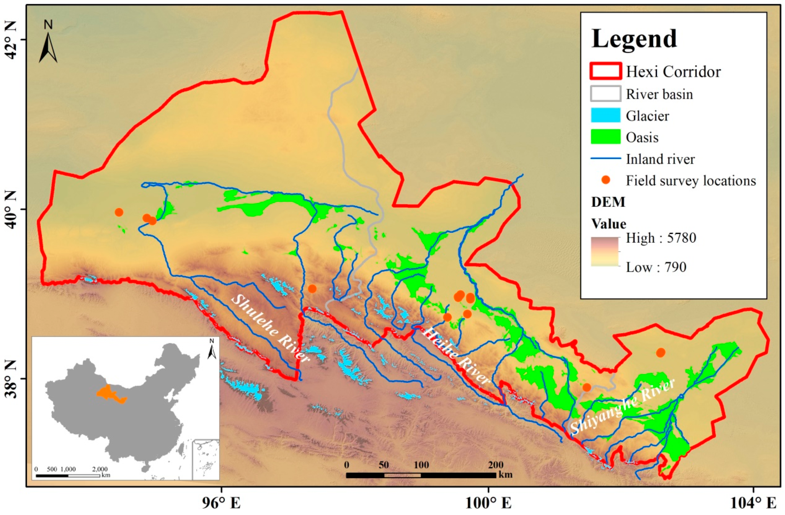
The Hexi Corridor (90°11′–101°29′ E, 37°14′–42°15′ N) is a belt region located in northwest China. The altitude of the study area ranges from 790 to 5780 m and the climate is arid, temperate monsoon, characterized by a hot summer and cold winter. The annual average temperature during the study period ranged from 4 to 10 °C, and the annual average precipitation was from 100 to 400 mm in the region, showing a decreasing trend from southeast to northwest. The region is comprised of three inland rivers, all originated from the Qinghai-Tibet Plateau, including the Shiyanghe river basin, the Heihe river basin, and the Shulehe river basin, distributing from southeast to northwest (Figure 1). Arable land in the study area is mainly distributed in the oases of the Jinchang, Minqin, Sunan, Wuwei, and Yongchang administrative counties in the Shiyanghe river basin; in Gaotai, Jiayuguan, Jinta, Jiuquan, Linze, Minle, Shandan, and Zhangye administrative counties in the Heihe river basin; and in Akesai, Dunhuang, Guazhou, Subei, and Yumen administrative counties in the Shulehe river basin. By thousands of years of cultivation, the arable land has differed clearly from other land use types, so we selected this region to examine the method for arable land extracting.
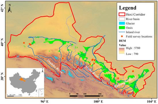
Figure 1.
Location of the study area.
2.2. General Prodcedure of Data Processing
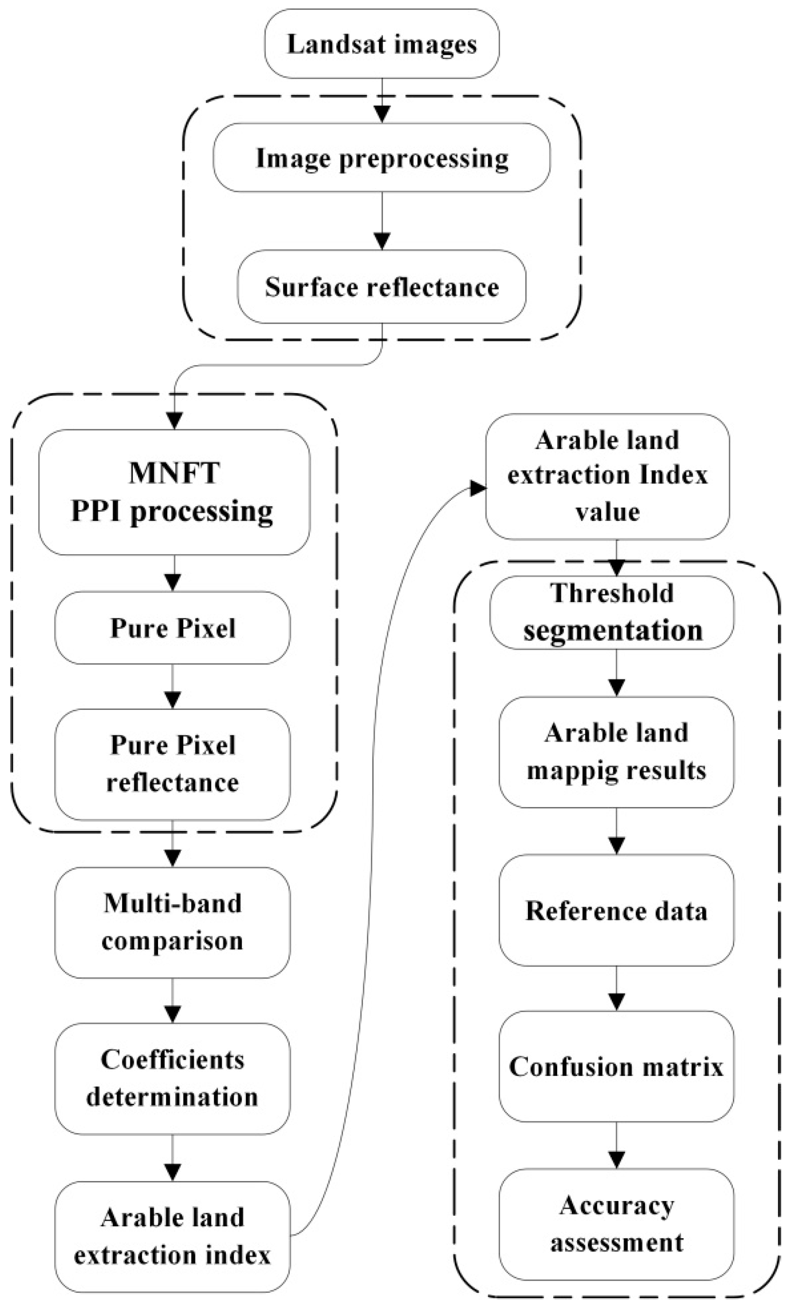
The arable land was extracted in four successive steps (Figure 2): (1) data selection and processing, (2) pure pixels’ selection, (3) index framework setup, and (4) arable land extracting and accuracy estimation.

Figure 2.
Workflow chart of arable land extraction.
2.2.1. Data Sources and Preprocessing
A total of 40 Landsat images (10 images for each year, see Appendix A) were collected for the years 1990, 2000, 2010, and 2020. The Landsat-series images covered seven paths from east to west (131–137) and three rows from north to south (032–034) and contained 30 Landsat-5 TM and 10 Landsat-8 OLI images acquired in the summer season. The Google Earth Engine [21,29] was used to identify the images that were cloud-free and possessed the highest crop coverage rates through the years. Thus, 40 raw format images acquired from 16 June to 6 September during the 30 years were selected and downloaded from the public domain of the Earth Resources Observatory and Science Center (EROS, http://eros.usgs.gov, accessed on 18 October 2020) using a Python bulk download application. The images were then rectified to the Universal Transverse Mercator (UTM) projection using at least 45 well-distributed ground control points (GCPs) and nearest neighborhood resampling method for each image, and the root mean square error (RMSE) was set to be less than 1 pixel. Radiometric calibration, fast line-of-sight atmospheric analysis of spectral hypercubes (FLAASH) atmospheric correction, and geometry correction were conducted to obtain surface reflectance images using a batch-processing IDL program.
2.2.2. Selection of Pure Pixels
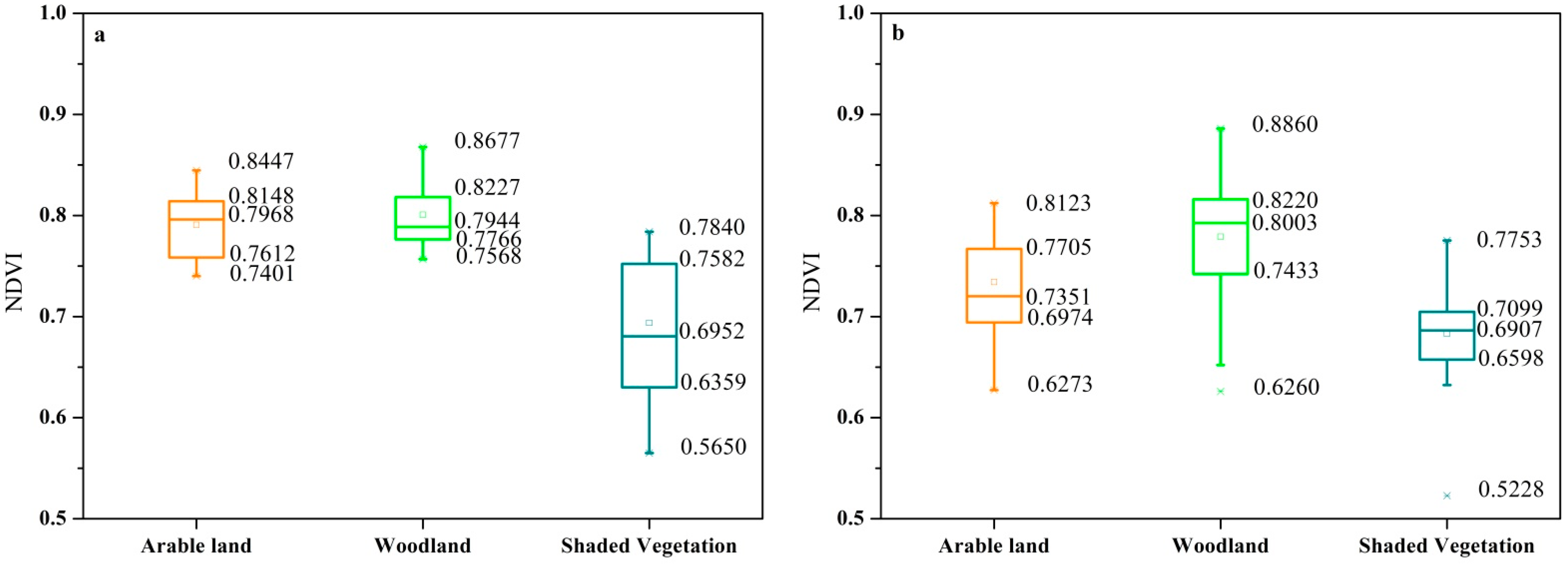
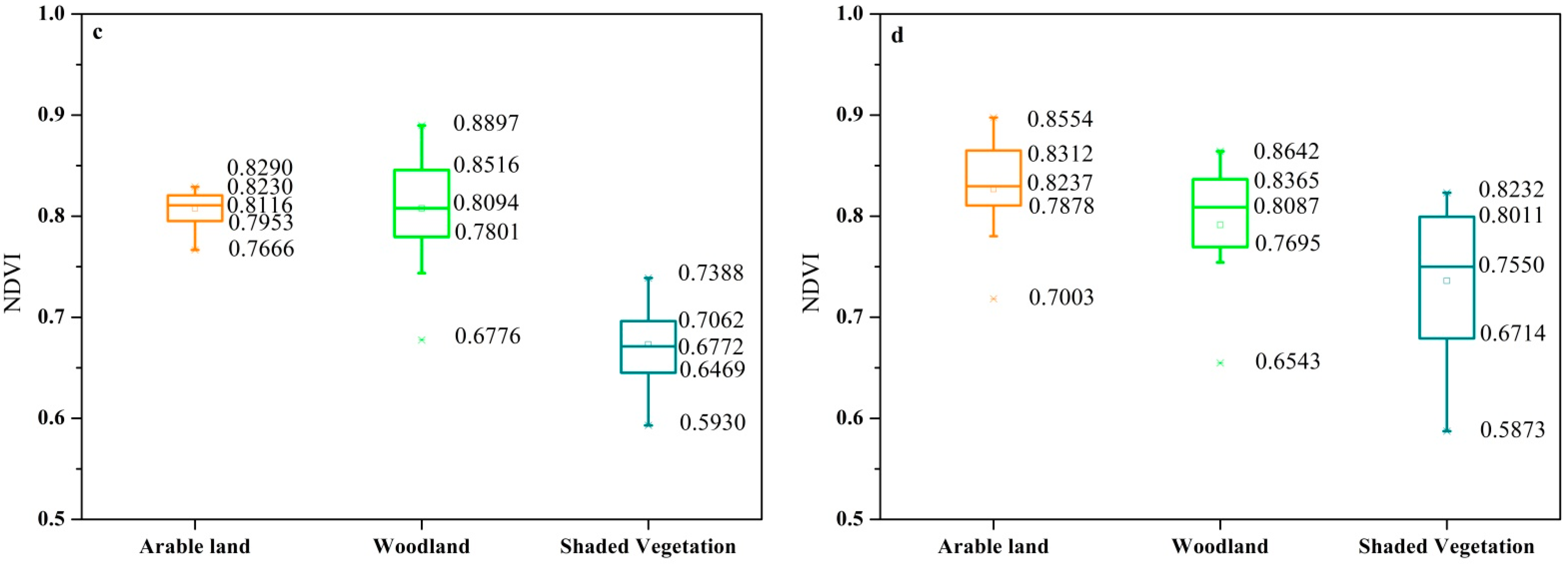
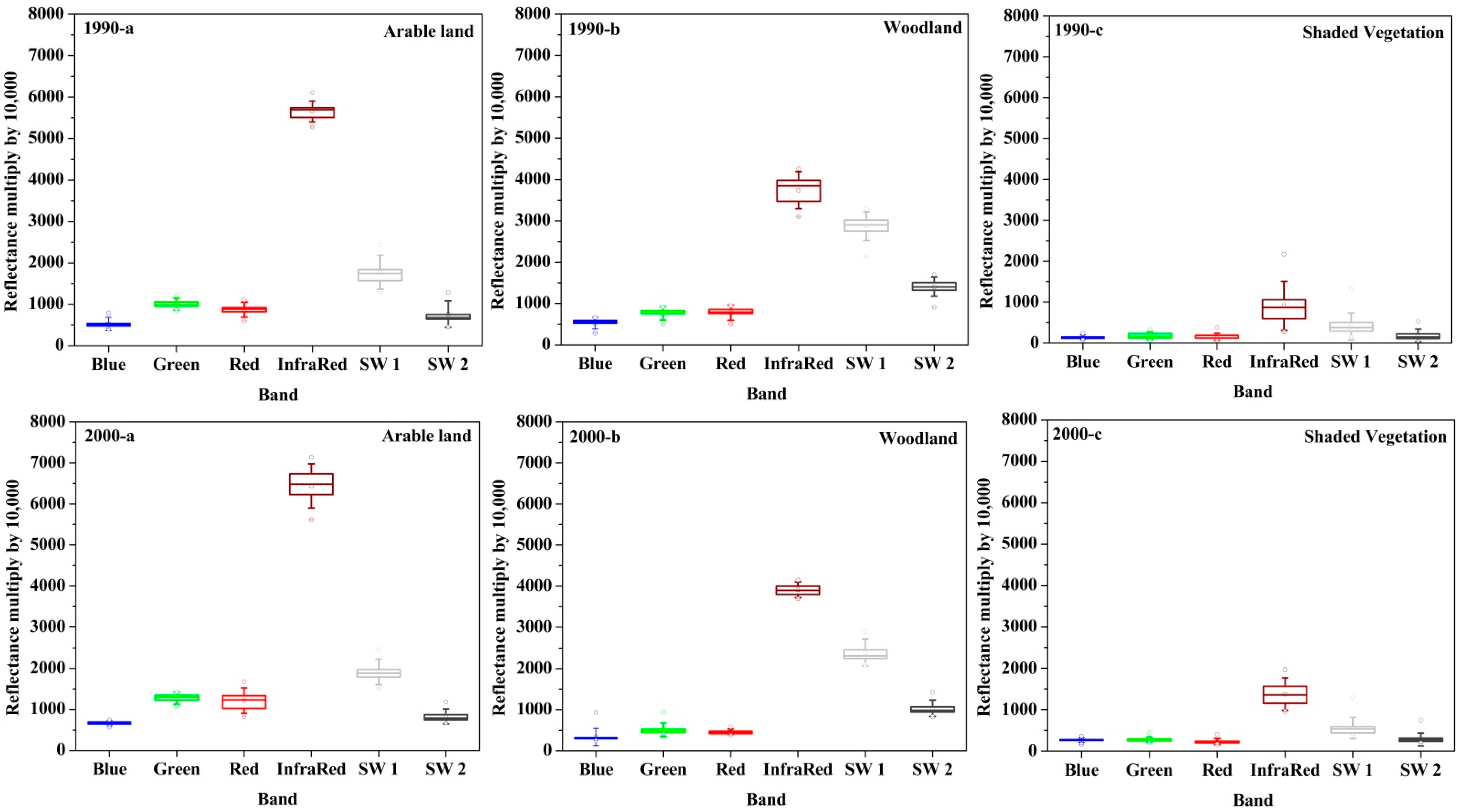
Owing to the high separability characteristics between vegetation (arable land, woodland, etc.) and other land use/cover types (desert, urban and rural areas, glacier, waterbody, etc.), the NDVI threshold method can be used to distinguish and locate vegetation areas in the remotely sensed images. However, due to apparent overlaps in the reflectance and impact of terrain fluctuation, arable land is hard to be accurately separated from woodland and shaded vegetation based on NDVI differences (Figure 3). Here the three land use/cover types (arable land, woodland, and shaded vegetation) were visually interpreted from five randomly selected Landsat images for each year with the aid of Google Earth Pro images, and their NDVI values were calculated using the equation below.
where NIR represents the reflectance value of Near-infrared band, and R is the reflectance value of Red band.
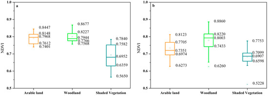
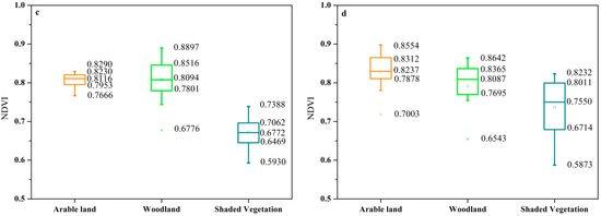
Figure 3.
NDVI distributions of arable land, woodland, and shaded vegetation in the Landsat images in the year 1990 (a), 2000 (b), 2010 (c), and 2020 (d). The three land use/cover types were visually interpreted from the randomly selected Landsat images with the aid of Google Earth Pro images. Each box plot explains the location of the 0th, 25th, 50th, 75th, and 100th percentiles using horizontal lines (boxes and whiskers).
The Minimum Noise Fraction Transform (MNFT) and Pixel Purity Index (PPI) were conducted on the Landsat images to find pure pixels, which were used to detect cues of spectral difference between arable land and other vegetation types [30,31]. At first, the MNFT was used to eliminate the noise in the images by principal component transformations in two steps. The first transformation (based on the estimated noise covariance matrix) was to separate and re-adjust the noise in the data, by minimizing the variance of the transformed noise data without correlation between bands. The second step was to transform the standard principal component of the noise-whitened data [32].
The pixel purity index (PPI) has been widely used in multi-spectral image analysis for pure pixel detection. After the MNFT processing, a set of k unit vectors was generated, where k is a sufficiently large, positive integer. For each , all the data sample vectors were projected onto to find sample vectors at its extreme positions to form an extrema set for this particular , denoted by Sextrema(). Despite the fact that a different generates a different extrema set Sextrema(), it is likely that some sample vectors may appear in more than one extrema set. Define an indicator function of a set S, IS(r) by
where is defined to be the PPI score of sample vector [33]. A large PPI value (e.g., 1) indicates a high possibility of a pure pixel [34].
The pixels with high PPI values were then exported to establish a new region of interest (ROI) and then linked to the Google Earth Pro images (0.5-m spatial resolution) to further examine the purity of these pixels. Finally, about 400 pure pixel samples were selected in each image for further analysis.
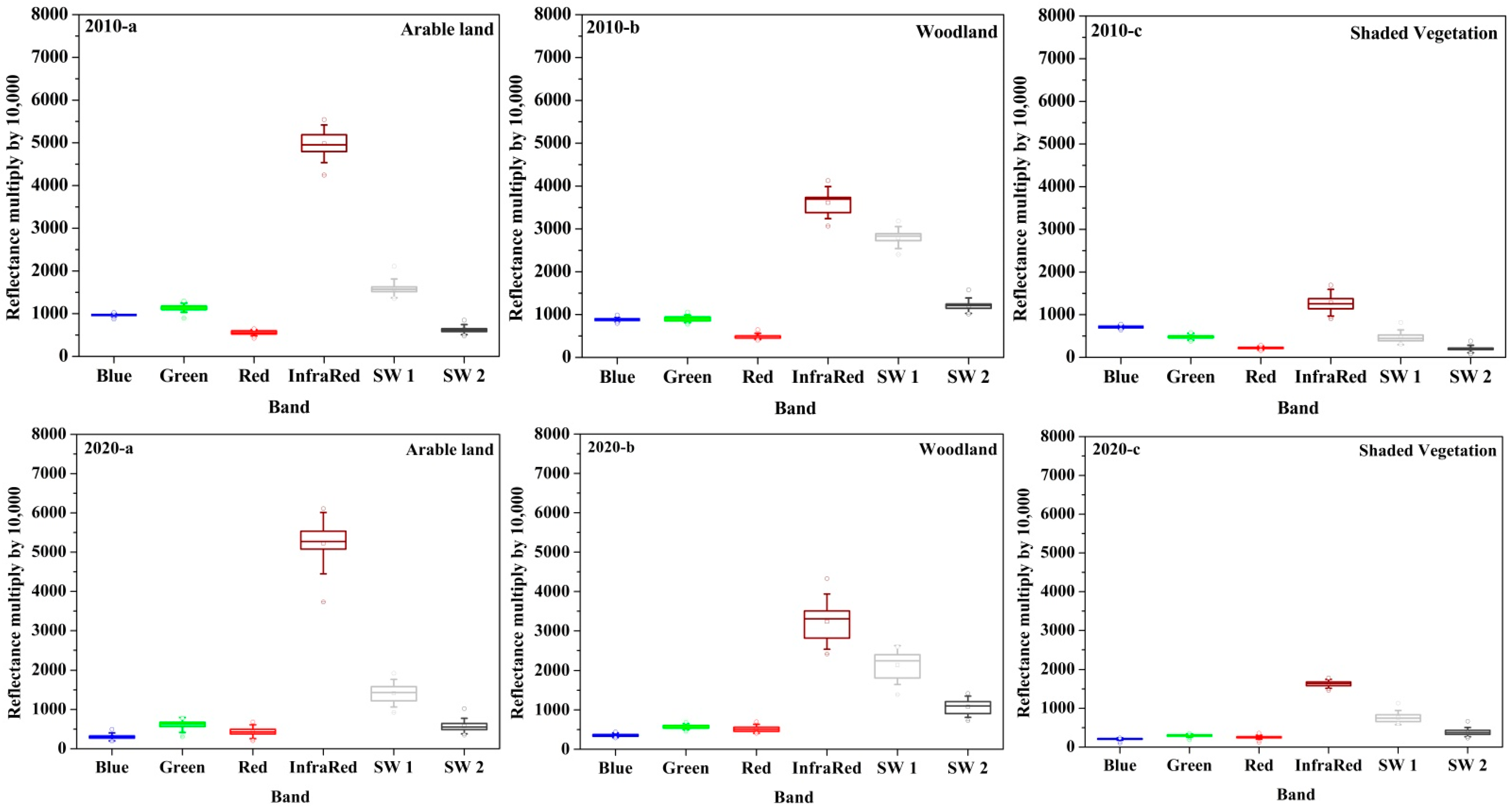
Figure 4 shows the reflectance of the six bands (Blue, Green, Red, Infrared, shortwave 1, and shortwave 2) of the p132r34 image as an example. Comparison analysis found that the spectral change patterns of arable land, woodland, and shaded vegetation were similar to each other. However, the value of the Infrared band was apparently different from other bands and, thus, this band was selected as the basis to design the framework to distinguish arable land areas.
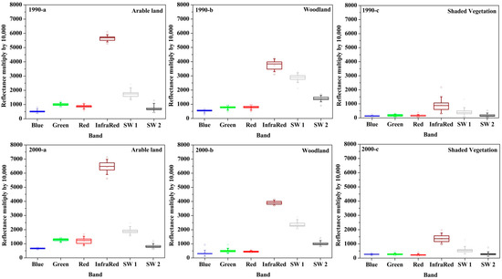
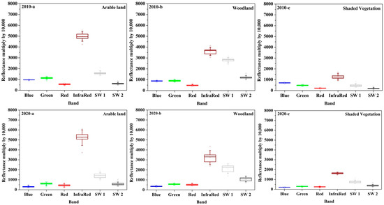
Figure 4.
Surface reflectance distributions of pure pixels of (a) arable land, (b) woodland, and (c) shaded vegetation in the example image. The reflectance value was multiplied by 10,000. Each box plot explains the location of the 0th, 25th, 50th, 75th, and 100th percentiles using horizontal lines (boxes and whiskers).
2.2.3. Formulation of Arable Land Extraction Index (ALEI)
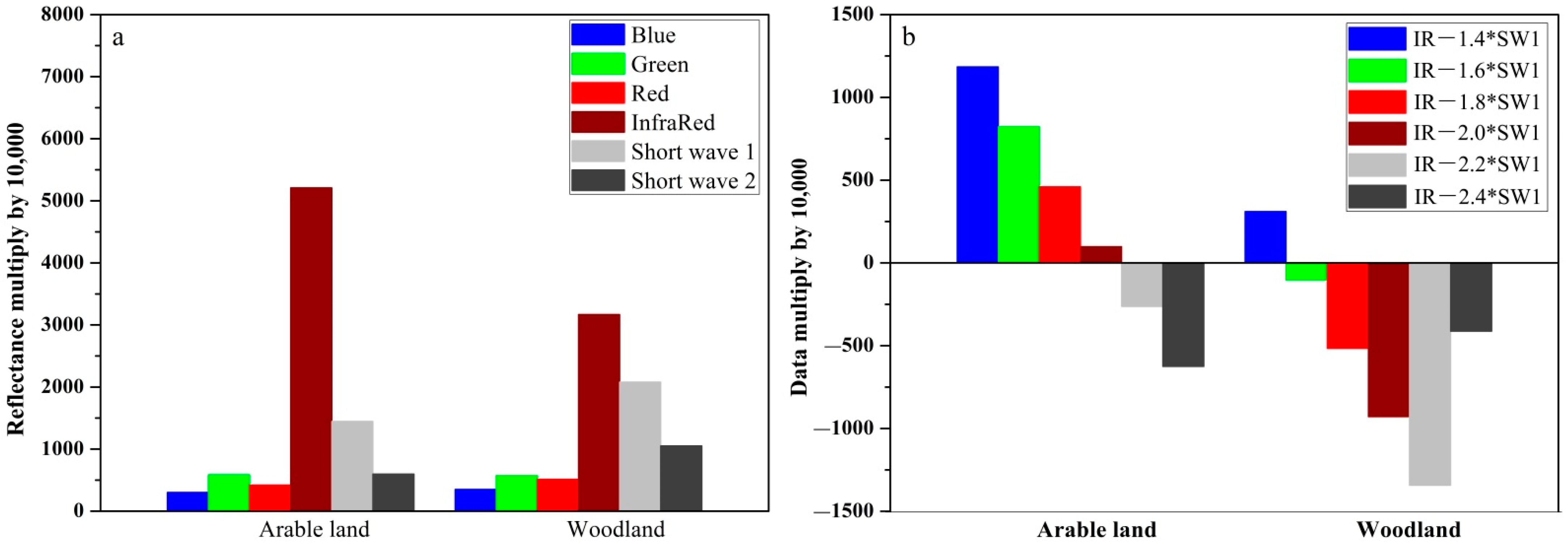
Spectral difference is an important foundation to discern arable land. As the wavelength increasing from visible to the shortwave bands, the reflectance of arable land and natural vegetation showed the same change pattern. They increased in the Green band, slightly decreased in the Red band, significantly increased in the Infrared band, and then decreased in the Shortwave bands (Figure 4). The shaded vegetation shared the same change pattern with that of woodland but the reflectance in the Infrared was much less than those of arable land and woodland (Figure 4) and the other images shared the same spectral distribution characteristics. This can help separate shaded vegetation and eliminate its impact on arable land extract. Therefore, the main issue was to separate arable land from woodland in the agro-pastoral zones. After analyzing the spectral change patterns of arable land and woodland, the Infrared and Shortwave 1 were selected to form an arable land extraction index to maximize the contrast between arable land and woodland.
where is the reflectance value of the Infrared band and is the reflectance value of the first shortwave band.
For successive identification of arable land by excluding other easily confused land use/cover types, the key is to determine the coefficient ω to maximize the difference between arable land and natural vegetation. So, iteration computations with different ω values were conducted, and the results are presented in Figure 5b. Considering the image acquisition date and land use/cover distribution in the study area, the value cannot be too small or too large, as such may lower the desired difference to separate arable land and woodland. For instance, if ω were 1.4, the index values for the two land use/cover types are positive, and when the ω value increases, e.g., to larger than 2.2, their values become negative. By iterative examinations, the suitable ω value can be set to 1.6 or 2.0 for the formula, but they both fail to fulfill the purpose of maximizing the difference between arable land and woodland. By assigning the coefficient ω to be 1.8, the pixel with positive index value represents arable land and the pixel-processing negative one is woodland. Here, we consented that 0 was a default threshold for separating arable land from woodland, because pixels with positive and negative ALEI values are easier to be classified into different land use/cover categories.
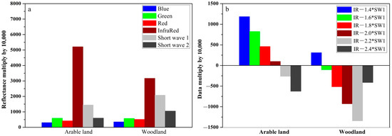
Figure 5.
Process of arable land extraction index formation. (a) Average reflectance of the six bands in the Landsat images; (b) a process of determining the optimal coefficients of the proposed index.
2.2.4. Verification
After the determination of ω parameter, the ALEI was applied to extract the arable land. The arable land extraction framework was built using a two-branch decision tree method. At first, “B1 LT 2500” was used to eliminate the impact of shaded vegetation to arable land extraction, where “B1” is the abbreviation of Band 1, i.e., the Infrared bands of Landsat image, and “LT” represents “Less Than”, i.e., the pixels in the Landsat images with Infrared value of less than 0.25 that were classified to shaded vegetation. Secondly, the remaining pixels were further processed using the “B2 GT 1.8” to distinguish arable land, in which the “B2” (Band 2) is the ALEI-based results calculated using Equation (3) and “GT” is the abbreviation of “Greater Than”. The pixels with ALEI values greater than 1.8 were grouped into the arable land class. In this study, 40 decision trees were established separately and 40 different B1 and B2 sets were used to obtain the computation results.
A 160,000-pixel ground truth data set was randomly selected, and the land use types for each image were visually interpreted based on Google Earth Pro online images (0.5-m spatial resolution). With this ground truth data set, the currency of the ALEI-based results was examined using four coefficients, i.e., user’s accuracy, producer’s accuracy, overall accuracy, and Kappa coefficient [35]. The user’s accuracy is the ratio of the total number of pixels correctly classified into class i (diagonal value in the confusion matrix) and the total number of pixels classified into class i by the classifier (the sum of class i rows in the confusion matrix). The producer’s accuracy is the ratio of the number of pixels (diagonal value in the confusion matrix) that the classifier correctly classifies for the entire image into class i and the true total number of class i (the sum of class i columns in the confusion matrix).
Furthermore, intensive field surveys were conducted for 15 arable land areas in July 2012 and July 2020, for each of which the arable land area boundary was recorded by walking around it using a high-precision tracking GPS (position dilution of precision ≤4, error < 10 m). The recorded boundary for each of the 15 arable land areas was input into ArcGIS 10.6, and then the area was computed. These data were then used for in situ verification of the arable land area obtained from the ALEI method in 2010 and 2020, with the mean relative error (MRE) as below.
where is the ith area obtained from field survey, is the ith area from ALEI method, and is 15, the total number of the field survey locations.
2.3. Dynamic Change Monitoring of Arable Land
Arable land dynamic change during 1990–2000, 2000–2010, and 2010–2020 in the three river basins was computed by the equations below:
where is the net change rate index and is the status and change trend index. and are the total area of arable land in the initial and end year of the research period, and represent the area gained and lost during 1990–2020, respectively, and is the time duration of the time interval of 10 years. From the Equations (5) and (6), the higher the is, the more the overall growth is. When is less than 0, the total arable land is reduced; otherwise, it is increased.
3. Results and Discussion
3.1. Verification of Arable Land Extraction
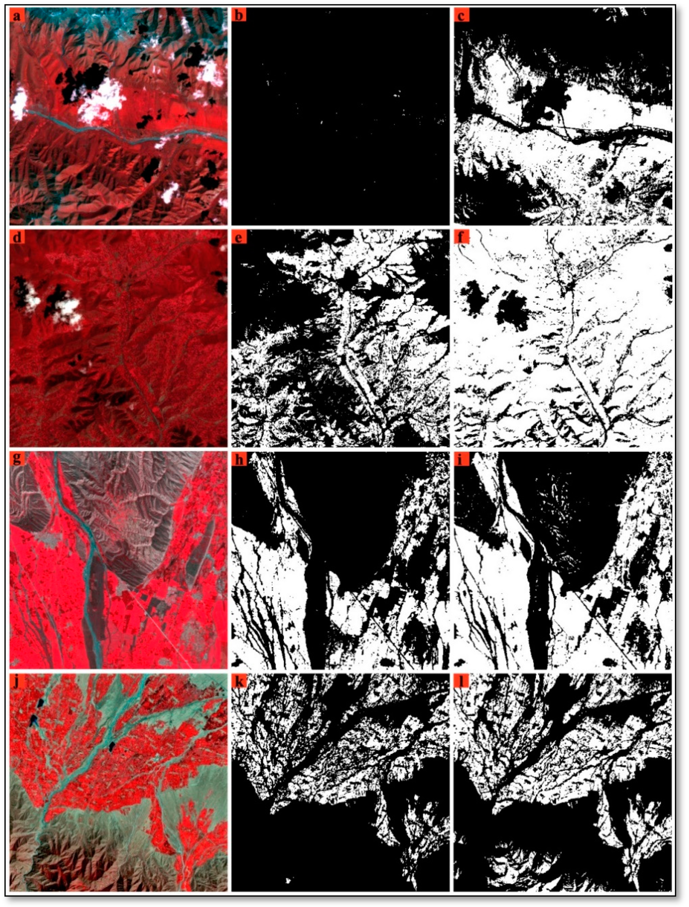
The overall accuracy (kappa coefficient) values of arable land extraction using the ALEI method all exceeded 0.89 (0.87), and both user’s and producer’s accuracies were higher than 0.84, indicating that the classification results were feasible for arable land change analysis (Table 1). Four 160,000-pixel zones were randomly selected in the images of p131r34, p132r34, p133r33, and p135r32 from southeast to northwest to visually show the extraction results. The original Landsat images, the arable land results using the ALEI and the NDVI threshold method, are shown in Figure 6. Both the ALEI and NDVI methods can distinguish vegetation from non-vegetation land use/cover types such as cloud, waterbody, riverbed, urban, and rural areas. However, NDVI-based method confused arable land areas with woodland and shaded vegetation (Figure 6f,l), which resulted in overestimation of arable land areas.

Table 1.
Accuracy assessment of arable land and other vegetation types.
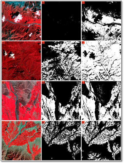
Figure 6.
Extraction results of arable land in representative agro-pastoral transition zones. (a) The p131r34 image acquired in 1990; (d) p132r34 image in 2000; (g) p133r33 image in 2010; (j) p135r32 image in 2020. Result map of (b,e,h,k): the extraction results based on the proposed ALEI method in this study; (c,f,i,l) the arable land areas from the NDVI threshold method. White areas represent extracted arable land and black ones are the other land cover types.
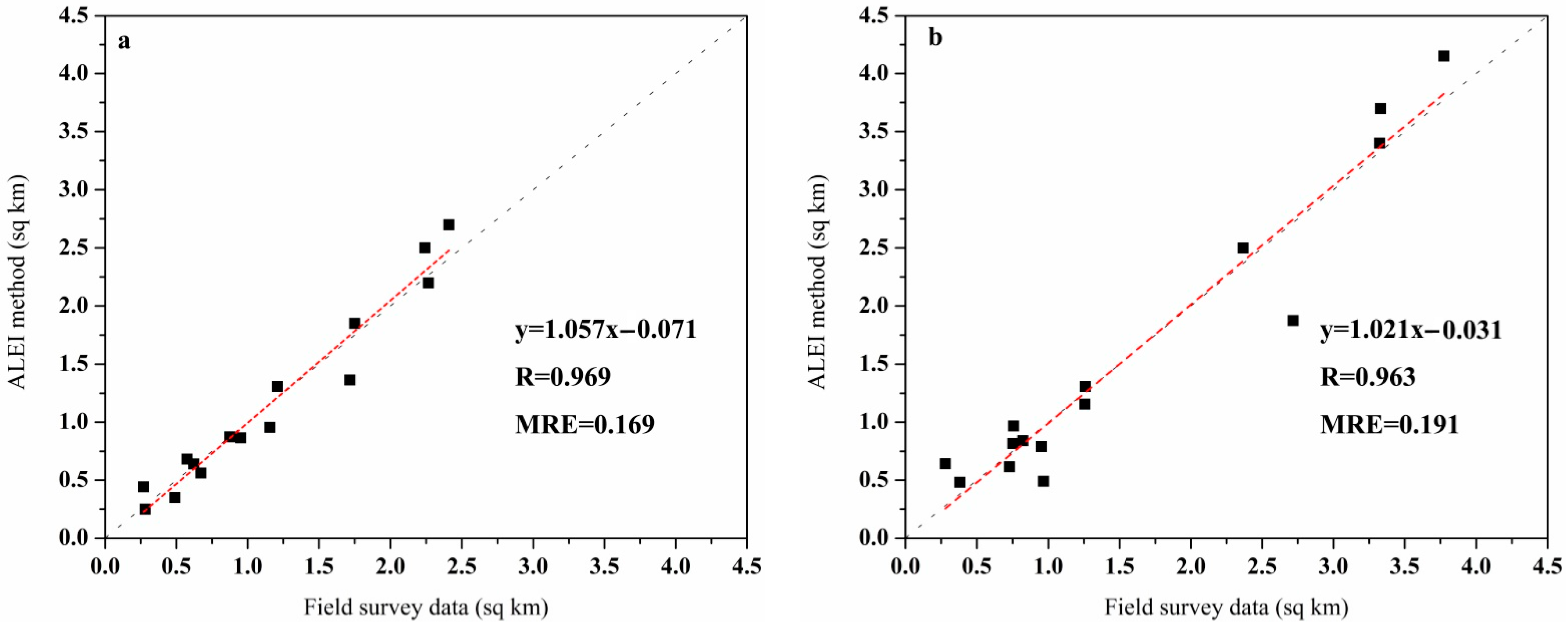
The accuracy of arable land extraction was further verified using areas of arable land obtained in the field survey in the summer season of 2012 and 2020. The correlation between field survey data and ALEI-based data are shown in Figure 7. Both the areas of arable land in 2010 and 2020 showed a high correlation, the coefficients of the years 2010 and 2020 were 0.969 and 0.963, and the MRE values were 0.169 and 0.191, respectively. However, the ALEI results were slightly overestimated compared to the field survey data. This was mainly attributed to the mixing pixels existing in these Landsat images. For instance, a pixel that contained 80% arable land and 20% other land use/cover types was classified as arable land using the ALEI method, resulting in some error. Overall, the classification accuracy using the ALEI method was acceptable and the results can be used to monitor the dynamic change of arable land in the study area.
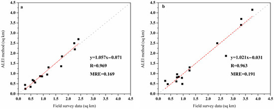
Figure 7.
Estimates of arable land using the ALEI method vs. field survey data obtained in 2010 (a) and 2020 (b).
3.2. Change Pattern of Arable Land in the Study Area
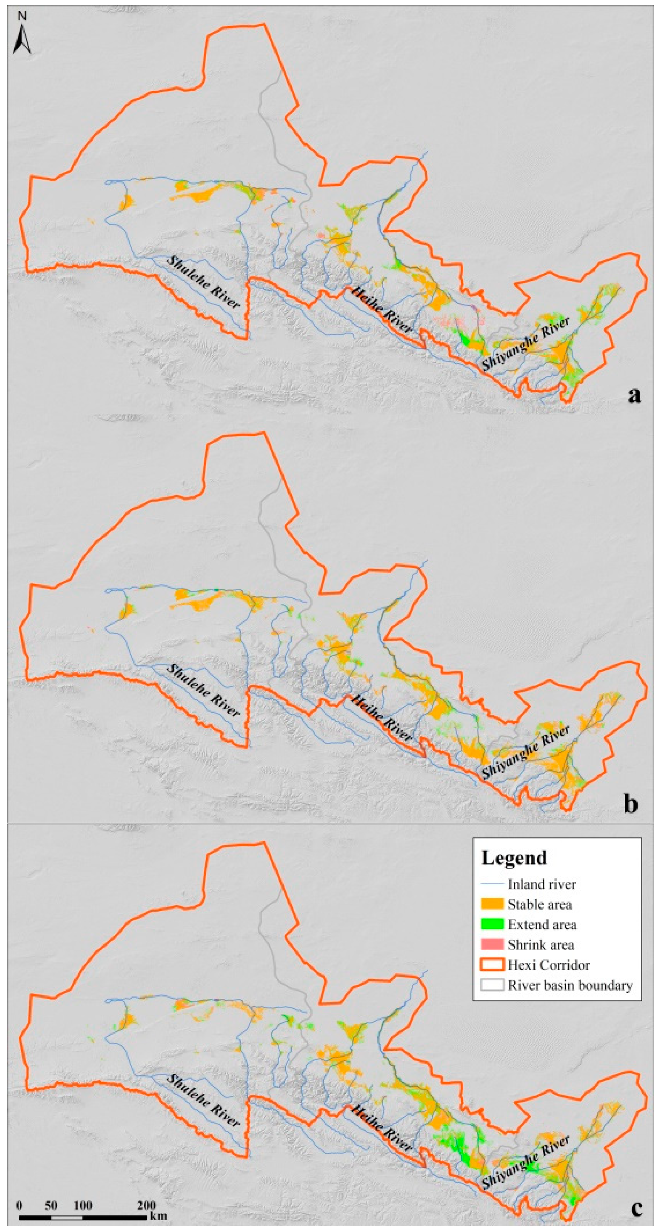
The extracted arable land in the study area during 1990–2020 are presented in Figure 8. In 1990, the total area of arable land was 10,546.33 km2, of which 34.45%, 46.42%, and 19.13% was distributed in the Shiyanghe, the Heihe, and the Shulehe river basins, respectively. In 2020, the total arable land area was 13,217.58 km2, increased by 25.33% compared to that in 1990, which reached its extreme value. During the three 10-year study intervals, arable land in the Hexi Corridor showed a continually increasing trend with the increase rates of 4.99%, 10.86%, and 7.43%, respectively. The most significant increase occurred during 2000–2010.
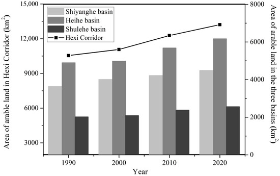
Figure 8.
Oasis change in the Hexi Corridor during 1990–2020. The black, block line shows the change trend of arable land area, and the bars indicate the arable land area of the Shiyanghe, Heihe, and Shulehe inland river basins.
In the three inland river basins, arable land showed a significantly expanding trend during the whole study period, while they showed different change patterns in the three 10-year intervals:
- 1.
- In the Shiyanghe river basin, arable land area increased rapidly with an annual rate of 2.36 % from 1990 to 2020, which was the lowest among the three inland river basins (Heihe river basin 2.60%/year, Shulehe river basin 2.68%/year). In this river basin, the most rapid arable land expansion occurred during 1990–2000, with a net change rate of 0.99%. The trend index of this 10-year interval was 0.51. It had not much difference with the other two 10-year periods (0.53 during 2000–2010 and 0.50 in 2010–2020 interval, Table 2). This indicated that, though arable land in the Shiyanghe basin expanded prominently, the area lost was also significant (Figure 9).
 Table 2. Change of arable land in the three 10-year intervals.
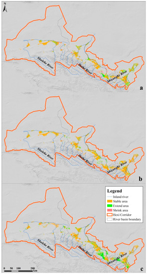 Figure 9. Arable land change in the study area during the three 10-year intervals. (a) 1990–2000; (b) 2000–2010; (c) 2010–2020.
- 2.
- Arable land in the Heihe river basin during 1990–2000 extended slightly in area (0.17 %/year), and the peak cumulative period of arable land occurred in the second 10-year interval (2000–2010, Figure 9). The area of arable land went up to 5681.04 km2 with the net change rate of 1.33 % and trend index of 0.82, both of which were the highest among the three river basins. During 2010–2020, arable land in the Heihe river basin accumulated another 488.15 km2, and the net change rate and trend index showed a decrease trend compared to those in the second 10-year interval (Table 2).
- 3.
- Arable land area of the Shulehe river basin in 1990 (2017.87 km2) only accounted for 55.55% and 41.22 % of that in the Shiyanghe and Heihe basins, respectively. However, arable land in the Shulehe river basin showed a similar change trend with that in the Heihe river basin (Figure 8 and Table 2). During 2000–2010, the area of arable land in the Shulehe basin increased by 292.12 km2 (14.09 %) and during 2010–2020, it further expanded by 7.61 % (Figure 9).
3.3. Discussion
This study established a framework to distinguish arable land and its change patterns in the Hexi Corridor, northwest China. The ALEI method was proposed to distinguish arable land based on 40 Landsat series images. The results demonstrated that the ALEI method is a feasible tool for extracting arable land areas accurately. The arable land in the study area showed an ongoing, expanding trend during 1990–2020, while the three inland river basins experienced different change patterns among the three 10-year intervals.
Compared to the NDVI threshold method, ALEI can help distinguish arable land in the study area more accurately, especially in the agro-pastoral zones. The verification results demonstrated that the producer’s accuracy of arable land extraction using the ALEI method ranged from 0.88 to 0.94, which increased by 6.02% to 13.25% compared to that of the Globeland30 (0.8315) [28]. The study results revealed the status and change patterns of arable land in the Hexi Corridor and can be used as references for decision makers to implement more targeted land protection policies and regulations, to balance the socioeconomic and ecological conflicts.
The ALEI method uses an efficient process framework in which the works can be all or semi-automatically conducted, i.e., ALEI can be computed with a batch-processing module automatically, after the Landsat images are downloaded using a bulk download application. Overall, the proposed methodology is understandable and easy to use. As artificial oases in arid regions share similar vegetation types and Landsat image is one of the most popular remotely sensed data sets covering most of the arid regions worldwide [36], ALEI is a promising tool to accurately extract arable land for land use planning in other arid regions. However, there are some limitations that were noted. Firstly, the field surveys for the verification was limited, covering an area of less than 4 km2, because large arable land areas are hard to be measured using the “walking-GPS” way. Recently, an unmanned aerial system (UAS) was applied in the remote sensing studies [37,38] to measure large, arable land areas as the ground truth data. Considering that the field data in 2012 were collected by the “walking-GPS”, so the data in 2020 were also collected by the same way to maintain the consistency and minimize the uncertainties. Secondly, the ALEI method was used and tested in the Hexi Corridor, and more applications in other arid regions could be done to further examine its usability and accuracy.
4. Conclusions
This study developed, examined, and applied a framework and an index of ALEI to identify arable land and its change patterns during past decades in a representative arid region. The results demonstrated that the proposed framework can help identify arable land areas accurately and found that the arable land in the study area extended significantly during 1990–2020. The findings of this study offer essential data to support the formulation and implementation of arable land protection and development policies.
Author Contributions
Conceptualization, X.Y. and X.Z.; data analysis, X.Y. and Y.H.; investigation, X.L.; methodology, Y.H.; writing—original draft, X.Y.; review and editing, Y.H., C.L. and X.Z. All authors have read and agreed to the published version of the manuscript.
Funding
This research was funded by the Open fund of Key Laboratory of Land Surface Pattern and Simulation, Chinese Academy of Sciences, grant number LBKF201802. The APC was funded by the Open fund of Key Laboratory of Land Surface Pattern and Simulation, Chinese Academy of Sciences, grant number LBKF201802. The funders had no role in the study design, data collection and analysis, decision to publish, or preparation of the article.
Institutional Review Board Statement
Not applicable.
Data Availability Statement
The data used to support the findings of this study are available from the corresponding author upon request.
Acknowledgments
The authors would like to thank the editors and reviewers for helpful comments.
Conflicts of Interest
The authors declare no conflict of interest.
Appendix A

Table A1.
Metadata of Landsat images covering the oases in the study area.
Table A1.
Metadata of Landsat images covering the oases in the study area.
| Landsat ID | 1990 | 2000 | 2010 | 2020 | ||||
|---|---|---|---|---|---|---|---|---|
| Sensor | Acquisition Date | Sensor | Acquisition Date | Sensor | Acquisition Date | Sensor | Acquisition Date | |
| p131r33 | TM | 22 June 1990 | TM | 19 July 2000 | TM | 15 July 2010 | OLI | 10 July 2020 |
| p132r33 | TM | 1 September 1990 | TM | 11 August 2000 | TM | 23 August 2010 | OLI | 17 July 2020 |
| p132r34 | TM | 1 September 1990 | TM | 11 August 2000 | TM | 8 September 2010 | OLI | 17 July 2020 |
| p133r33 | TM | 23 August 1990 | TM | 18 August 2000 | TM | 14 August 2010 | OLI | 9 August 2020 |
| p134r32 | TM | 30 August 1990 | TM | 8 July 2000 | TM | 21 August 2010 | OLI | 1 September 2020 |
| p134r33 | TM | 30 August 1990 | TM | 8 July 2000 | TM | 21 August 2010 | OLI | 1 September 2020 |
| p135r32 | TM | 21 August 1990 | TM | 29 July 2000 | TM | 27 July 2010 | OLI | 23 August 2020 |
| p136r32 | TM | 28 August 1990 | TM | 20 June 2000 | TM | 16 June 2010 | OLI | 30 August 2020 |
| P136r33 | TM | 28August 1990 | TM | 20 June 2000 | TM | 16 June 2010 | OLI | 30 August 2020 |
| p137r32 | TM | 19 August 1990 | TM | 13 July 2000 | TM | 9 July 2010 | OLI | 6 September 2020 |
References
- Chen, B.; Xiao, X.; Li, X.; Pan, L.; Doughty, R.; Ma, J.; Dong, J.; Qin, Y.; Zhao, B.; Wu, Z.; et al. A mangrove forest map of China in 2015: Analysis of time series Landsat 7/8 and Sentinel-1A imagery in Google Earth Engine cloud computing platform. ISPRS J. Photogramm. Remote Sens. 2017, 131, 104–120. [Google Scholar] [CrossRef]
- Meyer, W.B.; Turner, B.L. Human Population Growth and Global Land-Use/Cover Change. Annu. Rev. Ecol. Syst. 1992, 23, 39–61. [Google Scholar] [CrossRef]
- Guo, Y.; Shen, Y. Agricultural water supply/demand changes under projected future climate change in the arid region of northwestern China. J. Hydrol. 2016, 540, 257–273. [Google Scholar] [CrossRef]
- Manjaribe, C.; Frasier, C.L.; Rakouth, B.; Louis, E.E. Ecological Restoration and Reforestation of Fragmented Forests in Kianjavato, Madagascar. Int. J. Ecol. 2013, 2013, 1–12. [Google Scholar] [CrossRef]
- Li, X.; Shao, M.; Zhao, C.; Jia, X. Spatial variability of soil water content and related factors across the Hexi Corridor of China. J. Arid. Land 2019, 11, 123–134. [Google Scholar] [CrossRef]
- Liu, F.; Yang, Y.; Shi, Z.; Storozum, M.J.; Dong, G. Human settlement and wood utilization along the mainstream of Heihe River basin, northwest China in historical period. Quat. Int. 2019, 516, 141–148. [Google Scholar] [CrossRef]
- Gloaguen, R.; Goerner, A.; Makeschin, F. Monitoring of the Ecuadorian mountain rainforest with remote sensing. J. Appl. Remote Sens. 2007, 1, 013527. [Google Scholar] [CrossRef]
- Li, Y.; Ge, Q.; Wang, H.; Liu, H.; Tao, Z. Relationships between climate change, agricultural development and social stability in the Hexi Corridor over the last 2000 years. Sci. China Earth Sci. 2019, 62, 1453–1460. [Google Scholar] [CrossRef]
- Ma, L.; Cheng, W.; Qi, J. Coordinated evaluation and development model of oasis urbanization from the perspective of new urbanization: A case study in Shandan County of Hexi Corridor, China. Sustain. Cities Soc. 2018, 39, 78–92. [Google Scholar] [CrossRef]
- Benkhattab, F.Z.; Hakkou, M.; Bagdanavičiūtė, I.; El Mrini, A.; Zagaoui, H.; Rhinane, H.; Maanan, M. Spatial–temporal analysis of the shoreline change rate using automatic computation and geospatial tools along the Tetouan coast in Morocco. Nat. Hazards 2020, 104, 1–18. [Google Scholar] [CrossRef]
- Ku, C.-A. Exploring the Spatial and Temporal Relationship between Air Quality and Urban Land-Use Patterns Based on an Integrated Method. Sustainability 2020, 12, 2964. [Google Scholar] [CrossRef]
- Friedl, M.A.; McIver, D.K.; Baccini, A.; Gao, F.; Schaaf, C.; Hodges, J.C.F.; Zhang, X.Y.; Muchoney, D.; Strahler, A.H.; Woodcock, C.E.; et al. Global land cover mapping from MODIS: Algorithms and early results. Remote Sens Environ. 2002, 83, 287–302. [Google Scholar] [CrossRef]
- Kibret, K.S.; Marohn, C.; Cadisch, G. Use of MODIS EVI to map crop phenology, identify cropping systems, detect land use change and drought risk in Ethiopia–an application of Google Earth Engine. Eur. J. Remote Sens. 2020, 53, 176–191. [Google Scholar] [CrossRef]
- Loveland, T.R.; Reed, B.C.; Brown, J.F.; O Ohlen, D.; Zhu, Z.; Yang, L.; Merchant, J.W. Development of a global land cover characteristics database and IGBP DISCover from 1 km AVHRR data. Int. J. Remote Sens. 2000, 21, 1303–1330. [Google Scholar] [CrossRef]
- Gorelick, N. Google Earth Engine. In EGU General Assembly Conference Abstracts; American Geophysical Union: Vienna, Austria, 2013; Volume 15, p. 11997. [Google Scholar]
- Zhang, C.; Di, L.; Yang, Z.; Lin, L.; Hao, P. AgKit4EE: A toolkit for agricultural land use modeling of the conterminous United States based on Google Earth Engine. Environ. Model. Softw. 2020, 129, 104694. [Google Scholar] [CrossRef]
- Chen, C.; Wang, L.; Myneni, R.B.; Li, D. Attribution of Land-Use/Land-Cover Change Induced Surface Temperature Anomaly: How Accurate Is the First-Order Taylor Series Expansion? J. Geophys. Res. Biogeosci. 2020, 125. [Google Scholar] [CrossRef]
- Myroniuk, V.; Kutia, M.; Sarkissian, A.J.; Bilous, A.; Liu, S. Regional-Scale Forest Mapping over Fragmented Landscapes Using Global Forest Products and Landsat Time Series Classification. Remote Sens. 2020, 12, 187. [Google Scholar] [CrossRef]
- Patel, N.N.; Angiuli, E.; Gamba, P.; Gaughan, A.; Lisini, G.; Stevens, F.R.; Tatem, A.J.; Trianni, G. Multitemporal settlement and population mapping from Landsat using Google Earth Engine. Int. J. Appl. Earth Obs. Geoinf. 2015, 35, 199–208. [Google Scholar] [CrossRef]
- Dong, J.; Xiao, X.; Menarguez, M.A.; Zhang, G.; Qin, Y.; Thau, D.; Biradar, C.; Moore, B. Mapping paddy rice planting area in northeastern Asia with Landsat 8 images, phenology-based algorithm and Google Earth Engine. Remote Sens. Environ. 2016, 185, 142–154. [Google Scholar] [CrossRef]
- Gorelick, N.; Hancher, M.; Dixon, M.; Ilyushchenko, S.; Thau, D.; Moore, R. Google Earth Engine: Planetary-scale geospatial analysis for everyone. Remote Sens. Environ. 2017, 202, 18–27. [Google Scholar] [CrossRef]
- Wang, M.; Zhang, Z.; Hu, T.; Wang, G.; He, G.; Zhang, Z.; Li, H.; Wu, Z.; Liu, X. An Efficient Framework for Producing Landsat-Based Land Surface Temperature Data Using Google Earth Engine. IEEE J. Sel. Top. Appl. Earth Obs. Remote Sens. 2020, 13, 4689–4701. [Google Scholar] [CrossRef]
- Tang, L.; Zhao, M.; Wu, X. Accurate classification of epilepsy seizure types using wavelet packet decomposition and local detrended fluctuation analysis. Electron. Lett. 2020, 56, 861–863. [Google Scholar] [CrossRef]
- Wang, L.; Dong, Q.; Yang, L.; Gao, J.; Liu, J. Crop Classification Based on a Novel Feature Filtering and Enhancement Method. Remote Sens. 2019, 11, 455. [Google Scholar] [CrossRef]
- Xie, Y.; Bie, Q.; Lu, H.; He, L. Spatio-Temporal Changes of Oases in the Hexi Corridor over the Past 30 Years. Sustainability 2018, 10, 4489. [Google Scholar] [CrossRef]
- Venkatappa, M.; Sasaki, N.; Shrestha, R.P.; Tripathi, N.K.; Ma, H.-O. Determination of Vegetation Thresholds for Assessing Land Use and Land Use Changes in Cambodia using the Google Earth Engine Cloud-Computing Platform. Remote Sens. 2019, 11, 1514. [Google Scholar] [CrossRef]
- Brovelli, M.A.; Molinari, M.E.; Hussein, E.; Chen, J.; Li, R. The First Comprehensive Accuracy Assessment of GlobeLand30 at a National Level: Methodology and Results. Remote Sens. 2015, 7, 4191–4212. [Google Scholar] [CrossRef]
- Liu, J.; Peng, S.; Chen, J.; Liao, A.; Zhang, S. Knowledge-based method and engineering practice of globeland30 cultivated land data quality inspection. Bull. Surv. Mapp. 2015, 4, 42–48, (In Chinese with English Abstract). [Google Scholar]
- Martín-Ortega, P.; García-Montero, L.G.; Sibelet, N. Temporal Patterns in Illumination Conditions and Its Effect on Vegetation Indices Using Landsat on Google Earth Engine. Remote Sens. 2020, 12, 211. [Google Scholar] [CrossRef]
- Dadon, A.; Ben-Dor, E.; Karnieli, A. Use of Derivative Calculations and Minimum Noise Fraction Transform for Detecting and Correcting the Spectral Curvature Effect (Smile) in Hyperion Images. IEEE Trans. Geosci. Remote Sens. 2010, 48, 2603–2612. [Google Scholar] [CrossRef]
- Feyisa, G.L.; Meilby, H.; Fensholt, R.; Proud, S.R. Automated Water Extraction Index: A new technique for surface water mapping using Landsat imagery. Remote Sens. Environ. 2014, 140, 23–35. [Google Scholar] [CrossRef]
- Yu, K.-Q.; Zhao, Y.-R.; Liu, Z.-Y.; Li, X.-L.; Liu, F.; He, Y. Application of Visible and Near-Infrared Hyperspectral Imaging for Detection of Defective Features in Loquat. Food Bioprocess Technol. 2014, 7, 3077–3087. [Google Scholar] [CrossRef]
- Chang, C.-I.; Plaza, A. A Fast Iterative Algorithm for Implementation of Pixel Purity Index. IEEE Geosci. Remote Sens. Lett. 2006, 3, 63–67. [Google Scholar] [CrossRef]
- Jensen, J.R. Introductory Digital Image Processing: A Remote Sensing Perspective (No. Ed. 2); Prentice-Hall Inc.: Upper Saddle River, NJ, USA, 1996; p. 379. [Google Scholar] [CrossRef]
- Tung, F.; LeDrew, E. The determination of optimal threshold levels for change detection using various accuracy. Photogramm. Eng. Remote Sens. 1988, 54, 1449–1454. [Google Scholar]
- Yang, X.; Pavelsky, T.M.; Allen, G.; Donchyts, G. RivWidthCloud: An Automated Google Earth Engine Algorithm for River Width Extraction from Remotely Sensed Imagery. IEEE Geosci. Remote Sens. Lett. 2019, 17, 217–221. [Google Scholar] [CrossRef]
- Ma, L.; Cheng, L.; Han, W.; Zhong, L.; Li, M. Cultivated land information extraction from high-resolution unmanned aerial vehicle imagery data. J. Appl. Remote Sens. 2014, 8, 83673. [Google Scholar] [CrossRef]
- Yang, C.; Xu, G.; Li, H.; Yang, D.; Huang, H.; Ni, J.; Li, X.; Xiang, X. Measuring the area of cultivated land reclaimed from rural settlements using an unmanned aerial vehicle. J. Geogr. Sci. 2019, 29, 846–860. [Google Scholar] [CrossRef]
Publisher’s Note: MDPI stays neutral with regard to jurisdictional claims in published maps and institutional affiliations. |
© 2021 by the authors. Licensee MDPI, Basel, Switzerland. This article is an open access article distributed under the terms and conditions of the Creative Commons Attribution (CC BY) license (https://creativecommons.org/licenses/by/4.0/).

