
A Hybrid Multi-Objective Optimizer-Based SVM Model for Enhancing Numerical Weather Prediction: A Study for the Seoul Metropolitan Area

 , ,
, ,  ,
, 
Abstract
:1. Introduction
- Developing a hybrid model (GWO-SVM) to improve the forecasting of the daily maximum and minimum air temperatures produced by the NWP model;
- The proposed optimizer model (GWO) is compared with benchmark optimizers regarding the prediction accuracy and stability of SVM algorithm;
- Examine the proposed model’s forecasting in comparison with other machine learning approaches.
2. Materials and Methods
2.1. Materials
2.2. Preliminaries
2.2.1. Support Vector Machine (SVM)
2.2.2. Multi-Objective Grey Wolf Optimizer
2.3. Proposed Approach
2.3.1. Data Preprocessing
- (a)
- Exploratory Data Analysis (EDA)
- (b)
- Removing the Outliers
- (c)
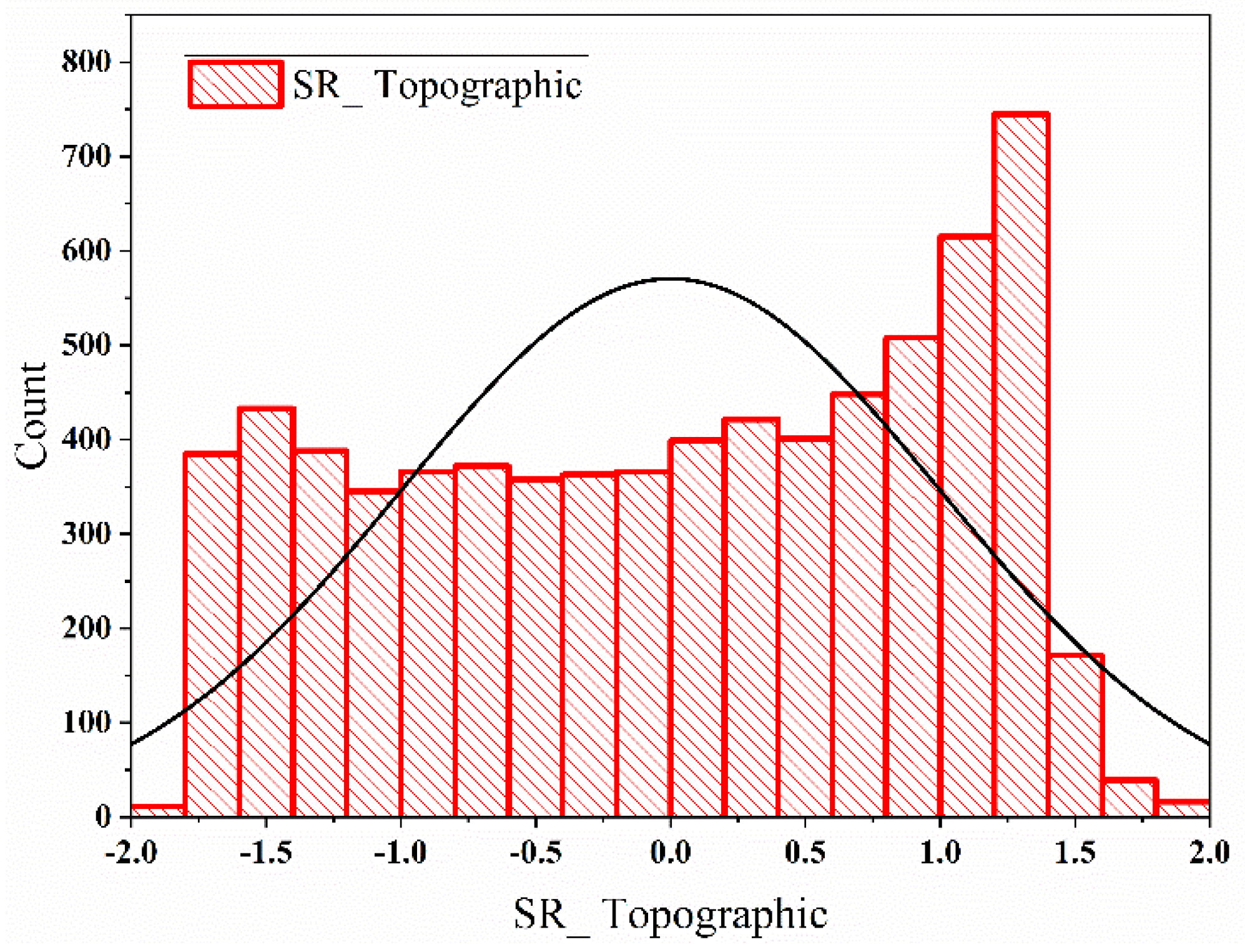
- Skewness Reduction
2.3.2. Development Regression Algorithm
2.3.3. Performance Analysis
3. Results and Discussion
4. Conclusions
Author Contributions
Funding
Institutional Review Board Statement
Informed Consent Statement
Data Availability Statement
Conflicts of Interest
References
- Alsharif, M.H.; Kim, J.; Kim, J.H. Opportunities and Challenges of Solar and Wind Energy in South Korea: A Review. Sustainability 2018, 10, 1822. [Google Scholar] [CrossRef] [Green Version]
- Alsharif, M.H.; Younes, M.K.; Kim, J. Time Series ARIMA Model for Prediction of Daily and Monthly Average Global Solar Radiation: The Case Study of Seoul, South Korea. Symmetry 2019, 11, 240. [Google Scholar] [CrossRef] [Green Version]
- Alsharif, M.H.; Younes, M.K. Evaluation and Forecasting of Solar Radiation using Time Series Adaptive Neuro-Fuzzy Inference System: Seoul City as A Case Study. IET Renew. Power Gener. 2019, 13, 1711–1723. [Google Scholar] [CrossRef]
- Durai, V.R.; Bhradwaj, R. Evaluation of statistical bias correction methods for numerical weather prediction model forecasts of maximum and minimum temperatures. Nat. Hazards 2014, 73, 1229–1254. [Google Scholar] [CrossRef]
- Goswami, K.; Hazarika, J.; Patowary, A.N. Monthly Temperature Prediction Based On Arima Model: A Case Study In Dibrugarh Station Of Assam, India. Int. J. Adv. Res. Comput. Sci. 2017, 8. [Google Scholar]
- Deif, M.A.; Solyman, A.A.A.; Hammam, R.E. ARIMA Model Estimation Based on Genetic Algorithm for COVID-19 Mortality Rates. Int. J. Inf. Technol. Decis. Mak. 2021, 1–24. [Google Scholar] [CrossRef]
- Candy, B.; Saunders, R.W.; Ghent, D.; Bulgin, C.E. The Impact of Satellite-Derived Land Surface Temperatures on Numerical Weather Prediction Analyses and Forecasts. J. Geophys. Res. Atmos. 2017, 122, 9783–9802. [Google Scholar] [CrossRef] [Green Version]
- Reichstein, M.; Camps-Valls, G.; Stevens, B.; Jung, M.; Denzler, J.; Carvalhais, N.; Prabhat. Deep learning and process understanding for data-driven Earth system science. Nature 2019, 566, 195–204. [Google Scholar] [CrossRef]
- Mirjalili, S.; Mirjalili, S.M.; Lewis, A. Grey wolf optimizer. Adv. Eng. Softw. 2014, 69, 46–61. [Google Scholar] [CrossRef] [Green Version]
- Anadranistakis, M.; Lagouvardos, K.; Kotroni, V.; Elefteriadis, H. Correcting temperature and humidity forecasts using Kalman filtering: Potential for agricultural protection in Northern Greece. Atmos. Res. 2004, 71, 115–125. [Google Scholar] [CrossRef]
- de Carvalho, J.R.P.; Assad, E.D.; Pinto, H.S. Kalman filter and correction of the temperatures estimated by PRECIS model. Atmos. Res. 2011, 102, 218–226. [Google Scholar] [CrossRef]
- Stensrud, D.J.; Yussouf, N. Short-Range Ensemble Predictions of 2-m Temperature and Dewpoint Temperature over New England. Mon. Weather. Rev. 2003, 131, 2510–2524. [Google Scholar] [CrossRef]
- Libonati, R.; Trigo, I.; DaCamara, C. Correction of 2 m-temperature forecasts using Kalman Filtering technique. Atmos. Res. 2008, 87, 183–197. [Google Scholar] [CrossRef]
- Cho, D.; Yoo, C.; Im, J.; Cha, D. Comparative Assessment of Various Machine Learning-Based Bias Correction Methods for Numerical Weather Prediction Model Forecasts of Extreme Air Temperatures in Urban Areas. Earth Space Sci. 2020, 7, e2019EA000740. [Google Scholar] [CrossRef] [Green Version]
- Chou, J.-S.; Pham, A.-D. Enhanced artificial intelligence for ensemble approach to predicting high performance concrete compressive strength. Constr. Build. Mater. 2013, 49, 554–563. [Google Scholar] [CrossRef]
- Healey, S.P.; Cohen, W.B.; Yang, Z.; Brewer, C.K.; Brooks, E.B.; Gorelick, N.; Hernandez, A.J.; Huang, C.; Hughes, M.J.; Kennedy, R.E.; et al. Mapping forest change using stacked generalization: An ensemble approach. Remote. Sens. Environ. 2018, 204, 717–728. [Google Scholar] [CrossRef]
- Ren, J.; Song, K.; Deng, C.; Ahlgren, N.A.; Fuhrman, J.A.; Li, Y.; Xie, X.; Poplin, R.; Sun, F. Identifying viruses from metagenomic data using deep learning. Quant. Biol. 2020, 8, 64–77. [Google Scholar] [CrossRef] [PubMed] [Green Version]
- Deif, M.A.; Hammam, R.E. Skin Lesions Classification Based on Deep Learning Approach. J. Clin. Eng. 2020, 45, 155–161. [Google Scholar] [CrossRef]
- Eccel, E.; Ghielmi, L.; Granitto, P.; Barbiero, R.; Grazzini, F.; Cesari, D. Prediction of minimum temperatures in an alpine region by linear and non-linear post-processing of meteorological models. Nonlinear Process. Geophys. 2007, 14, 211–222. [Google Scholar] [CrossRef] [Green Version]
- Yi, C.; Shin, Y.; Roh, J.-W. Development of an Urban High-Resolution Air Temperature Forecast System for Local Weather Information Services Based on Statistical Downscaling. Atmosphere 2018, 9, 164. [Google Scholar] [CrossRef] [Green Version]
- Deif, M.A.; Solyman, A.A.; Kamarposhti, M.A.; Band, S.S.; Hammam, R.E. A deep bidirectional recurrent neural network for identification of SARS-CoV-2 from viral genome sequences. Math. Biosci. Eng. 2021, 18, 8933–8950. [Google Scholar] [CrossRef]
- Marzban, C. Neural Networks for Postprocessing Model Output: ARPS. Mon. Weather. Rev. 2003, 131, 1103–1111. [Google Scholar] [CrossRef]
- Vashani, S.; Azadi, M.; Hajjam, S. Comparative Evaluation of Different Post Processing Methods for Numerical Prediction of Temperature Forecasts over Iran. Res. J. Environ. Sci. 2010, 4, 305–316. [Google Scholar] [CrossRef] [Green Version]
- Zjavka, L. Numerical weather prediction revisions using the locally trained differential polynomial network. Expert Syst. Appl. 2016, 44, 265–274. [Google Scholar] [CrossRef]
- Isaksson, R. Reduction of Temperature Forecast Errors with Deep Neural Networks—Reducering av Temperaturprognosfel med Djupa Neuronnätverk; Department of Earth Sciences, Uppsala University: Uppsala, Sweden, 2018. [Google Scholar]
- Dua, D.; Graff, C. {UCI} Machine Learning Repository. 2017. Available online: https://archive.ics.uci.edu/ml/datasets/Bias+correction+of+numerical+prediction+model+temperature+foreca (accessed on 10 October 2021).
- Suykens, J.A.K.; Vandewalle, J. Least Squares Support Vector Machine Classifiers. Neural Process. Lett. 1999, 9, 293–300. [Google Scholar] [CrossRef]
- Kucharski, A.J.; Russell, T.W.; Diamond, C.; Liu, Y.; Edmunds, J.; Funk, S.; Eggo, R.M.; Centre for Mathematical Modelling of Infectious Diseases COVID-19 Working Group. Early dynamics of transmission and control of COVID-19: A mathematical modelling study. Lancet Infect. Dis. 2020, 20, 553–558. [Google Scholar] [CrossRef] [Green Version]
- Yan, H.; Zhang, J.; Rahman, S.; Zhou, N.; Suo, Y. Predicting permeability changes with injecting CO2 in coal seams during CO2 geological sequestration: A comparative study among six SVM-based hybrid models. Sci. Total. Environ. 2020, 705, 135941. [Google Scholar] [CrossRef] [PubMed]
- Sadeghi, R.; Zarkami, R.; Sabetraftar, K.; Van Damme, P. Use of support vector machines (SVMs) to predict distribution of an invasive water fern Azolla filiculoides (Lam.) in Anzali wetland, southern Caspian Sea, Iran. Ecol. Model. 2012, 244, 117–126. [Google Scholar] [CrossRef]
- Zhao, L.-T.; Zeng, G.-R. Analysis of Timeliness of Oil Price News Information Based on SVM. Energy Procedia 2019, 158, 4123–4128. [Google Scholar] [CrossRef]
- Deif, M.A.; Solyman, A.A.A.; Alsharif, M.H.; Uthansakul, P. Automated Triage System for Intensive Care Admissions during the COVID-19 Pandemic Using Hybrid XGBoost-AHP Approach. Sensors 2021, 21, 6379. [Google Scholar] [CrossRef]
- Liu, M.; Cao, Z.; Zhang, J.; Wang, L.; Huang, C.; Luo, X. Short-term wind speed forecasting based on the Jaya-SVM model. Int. J. Electr. Power Energy Syst. 2020, 121, 106056. [Google Scholar] [CrossRef]
- Deif, M.A.; Hammam, R.E.; Solyman, A.A.A. Gradient Boosting Machine Based on PSO for prediction of Leukemia after a Breast Cancer Diagnosis. Int. J. Adv. Sci. Eng. Inf. Technol. 2021, 11, 508–515. [Google Scholar] [CrossRef]
- Mirjalili, S.; Saremi, S.; Mirjalili, S.M.; Coelho, L.D.S. Multi-objective grey wolf optimizer: A novel algorithm for multi-criterion optimization. Expert Syst. Appl. 2016, 47, 106–119. [Google Scholar] [CrossRef]
- Al-Tashi, Q.; Rais, H.M.; Abdulkadir, S.J.; Mirjalili, S.; Alhussian, H. A Review of Grey Wolf Optimizer-Based Feature Selection Methods for Classification. In Algorithms for Intelligent Systems; Springer: Berlin/Heidelberg, Germany, 2020; pp. 273–286. [Google Scholar]
- Akbari, E.; Rahimnejad, A.; Gadsden, S.A. A greedy non-hierarchical grey wolf optimizer for real-world optimization. Electron. Lett. 2021, 57, 499–501. [Google Scholar] [CrossRef]
- Zhang, Z.; Hong, W.-C. Application of variational mode decomposition and chaotic grey wolf optimizer with support vector regression for forecasting electric loads. Knowl. Based Syst. 2021, 228, 107297. [Google Scholar] [CrossRef]
- Deif, M.; Hammam, R.; Solyman, A. Adaptive Neuro-Fuzzy Inference System (ANFIS) for Rapid Diagnosis of COVID-19 Cases Based on Routine Blood Tests. Int. J. Intell. Eng. Syst. 2021, 14, 178–189. [Google Scholar] [CrossRef]
- Nyitrai, T.; Virág, M. The effects of handling outliers on the performance of bankruptcy prediction models. Socio-Econ. Plan. Sci. 2019, 67, 34–42. [Google Scholar] [CrossRef]
- Box, G.E.P.; Cox, D.R. An analysis of transformations. J. R. Stat. Soc. Ser. B 1964, 26, 211–243. [Google Scholar] [CrossRef]
- Lu, H.; Ma, X.; Ma, M. A hybrid multi-objective optimizer-based model for daily electricity demand prediction considering COVID-19. Energy 2021, 219, 119568. [Google Scholar] [CrossRef]


| Variable Type | Abbreviation (unit) | Description |
|---|---|---|
| The variable that predicted using LDAPS | Tmax_LDAPS (°C) | Maximum air temperature |
| Tmin_LDAPS (°C) | Minimum air temperature | |
| RHmax_LDAPS (%) | Maximum relative humidity | |
| RHmin_LDAPS (%) | Minimum relative humidity | |
| AWS_LDAPS (m/s) | Average wind speed | |
| LHF_LDAPS (W/m2) | average latent heat flux | |
| CC1_LDAPS (%) | The average cloud cover during the next day’s 6 h split (0–5 h) | |
| CC2_LDAPS (%) | The average cloud cover during the next day’s 6 h split (6–11 h) | |
| CC3_LDAPS (%) | The average cloud cover during the next day’s 6 h split (12–17 h) | |
| CC4_LDAPS (%) | The average cloud cover during the next day’s 6 h split (18–23 h) | |
| PPT1_LDAPS (%) | The next day’s precipitation averaged over six hours (0–5 h) | |
| PPT2_LDAPS (%) | The next day’s precipitation averaged over six hours (6–11 h) | |
| PPT3_LDAPS (%) | The next day’s precipitation averaged over six hours (12–17 h) | |
| PPT4_LDAPS (%) | The next day’s precipitation averaged over six hours (18–23 h) | |
| In situ data | T max_present(°C) | Present maximum air temperature |
| T min_present(°C) | Present minimum air temperature | |
| Auxiliary data | Lat_Location (°) | Latitude |
| Log_Location (°) | Longitude | |
| ELEV_Topographic (m) | Elevation | |
| Slop_Topographic (°) | Slope | |
| SR_Topographic (wh/m2) | Daily solar radiation |
| Tmax_Forecast | |||
| Year | LDAPS | MME | SVM-GWO |
| 2015 | 2.07 | 1.53 | 0.94 |
| 2016 | 2.15 | 1.45 | 0.93 |
| 2017 | 2.04 | 1.65 | 0.98 |
| Average RMSE | 2.09 | 1.54 | 0.95 |
| Tmin_Forecast | |||
| Year | LDAPS | MME | SVM-GWO |
| 2015 | 1.47 | 1.05 | 0.896 |
| 2016 | 1.43 | 1.03 | 0.856 |
| 2017 | 1.39 | 0.84 | 0.696 |
| Average RMSE | 1.43 | 0.97 | 0.82 |
Publisher’s Note: MDPI stays neutral with regard to jurisdictional claims in published maps and institutional affiliations. |
© 2021 by the authors. Licensee MDPI, Basel, Switzerland. This article is an open access article distributed under the terms and conditions of the Creative Commons Attribution (CC BY) license (https://creativecommons.org/licenses/by/4.0/).
Share and Cite
Deif, M.A.; Solyman, A.A.A.; Alsharif, M.H.; Jung, S.; Hwang, E. A Hybrid Multi-Objective Optimizer-Based SVM Model for Enhancing Numerical Weather Prediction: A Study for the Seoul Metropolitan Area. Sustainability 2022, 14, 296. https://doi.org/10.3390/su14010296
Deif MA, Solyman AAA, Alsharif MH, Jung S, Hwang E. A Hybrid Multi-Objective Optimizer-Based SVM Model for Enhancing Numerical Weather Prediction: A Study for the Seoul Metropolitan Area. Sustainability. 2022; 14(1):296. https://doi.org/10.3390/su14010296
Chicago/Turabian StyleDeif, Mohanad A., Ahmed A. A. Solyman, Mohammed H. Alsharif, Seungwon Jung, and Eenjun Hwang. 2022. "A Hybrid Multi-Objective Optimizer-Based SVM Model for Enhancing Numerical Weather Prediction: A Study for the Seoul Metropolitan Area" Sustainability 14, no. 1: 296. https://doi.org/10.3390/su14010296