Spatio-Temporal Modeling of Small-Scale Ultrafine Particle Variability Using Generalized Additive Models

Abstract

High-resolution measurements of ultrafine particle concentrations in ambient air are needed for the study of health human effects of long-term exposure. This work, carried out in the framework of the VIEPI project (Integrated Evaluation of Indoor Particulate Exposure), aims to extend current knowledge on small-scale spatio-temporal variability of Particle Number Concentration (PNC, considered a proxy of the ultrafine particles) at a local scale domain (1 km × 1 km). PNC measurements were made in the university district of San Lorenzo in Rome using portable condensation particle counters for 7 consecutive days at 21 sites in November 2017 and June 2018. Generalized Additive Models (GAMs) were performed in the area for winter, summer and the overall period. The log-transformed two-hour PNC averages constitute the response variable, and covariates were grouped by urban morphology, land use, traffic and meteorology. Winter PNC values were about twice the summer ones. PNC recorded in the university area were significantly lower than those observed in the external routes. GAMs showed a rather satisfactory result in order to capture the spatial variability, in accordance with those of other previous studies: variances were equal to 71.1, 79.7 and 84%, respectively, for winter, summer and the overall period.

1. Introduction

Several studies have assessed the health effects of particles in the ultrafine mode (PM_0.1). The main concern is related to their capability to go deeper into the lung, where they are retained longer than the coarser particles, leading to pulmonary inflammation and endothelial dysfunction [1]. Moreover, it has been shown that ultrafine particles (UFP) exposure led to coagulation change that can be a risk factor for hypertension and cardiovascular disease. Among others, they have been linked to diabetes and cancer as well as cerebral dysfunctions due to direct translocation to the brain through the olfactory nerve [1,2].

Since ultrafine particles contribute largely to the airborne total particle number concentration (PNC), it was often used as a proxy for PM_0.1 exposure studies [3,4,5].

The outdoor PNCs spatial and temporal variability assessment and related population exposure gradients are key topics in order to evaluate the related health effects.

Some studies have attempted to evaluate the PNC spatial variability at an urban scale using Land Use Regression models (LURs). The LURs have been applied to large urban areas such as Amsterdam [6], Vancouver [7], New Delhi [8], Boston [9], Toronto [10], Rome [11], Berlin [12], London [13] and El Paso [14] including, at times, also the surrounding municipalities. In other cases, the method has been extended to wider territories of Girona (Spain, [15]) to include the entire national territory (Switzerland, [16]; the Netherlands [17]). These studies were based on multiple regression between the concentrations measured in different points (usually ranging between 20 and 80) and spatial explanatory variables extracted within zones of influence around each monitoring site, mainly starting from the assumption that the functional link between the regressors and the response variable was linear.

Although LUR models can be effective tools for evaluating the spatial distribution of PNC, leading to the identification of high-resolution concentration domains, actually the hypothesis that the functional link between the regressors and the response variable is linear seems weak, also after the PNCs log transformation.

In particular, in urban areas it has been observed that the PNC shows much more pronounced variations than that of the mass concentration of PM₁₀ as the distance from the road increases [18,19,20], and that the nanometric fraction of UFP is predominant in the measurement sites close to road traffic or hot spots [21,22]. Indeed, several studies have identified an exponential decrease in PNC as the distance from the road increases, for the unobstructed topographic settings [23,24]. It was also found a relative maximum in the PNC for distances around 90 m from heavy traffic roads such as motorways and expressways [18,25]. Moreover, if not only long-term exposure must be taken into account, the temporal variability also has to be contemporarily assessed.

PNC, in the field of ultrafine particles, varies over time both due to the processes of formation and growth of particles [26,27,28] and as a function of meteorological and micrometeorological physical-chemical parameters [25,29,30,31,32,33]. The formation mechanism (nucleation) leads to the generation of new UFP in the atmosphere starting from gaseous compounds; the volumetric growth of UFP is linked both to the condensation of gases on the UFP surface or to their dissolution in the liquid film that covers the particles. The main removal processes reside in dry and wet deposition [27,28].

The relationship between PNC and the main meteorological variables has been generally described by complex, non-linear functions [25,34,35].

The Generalized Additive Models (GAMs), using smoothing functions, allow the evaluation of non-linear interactions between the covariates and the response variable even in the very frequent case in which there is no prior knowledge of the kind of functional bond [36,37].

The use of smoothing functions in place of deterministic functions based, in linear models, on the estimation of regression parameters, has produced excellent results in the analysis of complex ecological systems [38,39].

The use of splines as smoothing functions allows both for reproducing the global trend of the contribution that the covariate provides to the response variable and to better approximate any local trends in particular intervals of the domain of existence of the explanatory variable [34,40].

GAMs have been used to assess the temporal relationships between PNC measured at fixed sites and meteorological parameters, allowing for positive results in terms of statistical performance [34,35,41].

However, both LUR models and GAMs have been applied to local (representative of a neighborhood or suburb) or microscales (representative of individual roads) only in a few studies. At such small spatial scale, spatio-temporal assessment is particularly challenging due to highly heterogeneous conditions [42,43,44]. Actually, concentrations in small urban domain are strongly dependent on short-term traffic variability [45,46]. The configurations of building and streets can play a relevant role by modifying local airflow patterns [47,48,49].

To the best of the authors’ knowledge, only a few studies [12,50] have addressed the goal to capture and effectively represent UFP urban hotspots spatial variability at a local or microscale through statistical models.

The aim of our work, carried out in the framework of the VIEPI project (Integrated Evaluation of Indoor Particulate Exposure) [51], was to further extend the current knowledge on small-scale spatio-temporal variability of PNC at local scale domain (1 km × 1 km).

To this purpose, we developed empirical regression models, GAMs, accounting for seasonal and diurnal variability. We demonstrate quantitatively the modeling approach effectiveness, while the PNC variability main descriptors and their contribution to the PNC-explained variance were assessed. The complexity of local urban design features was also explored using GIS derived urban morphology explanatory variables.

2. Materials and Methods

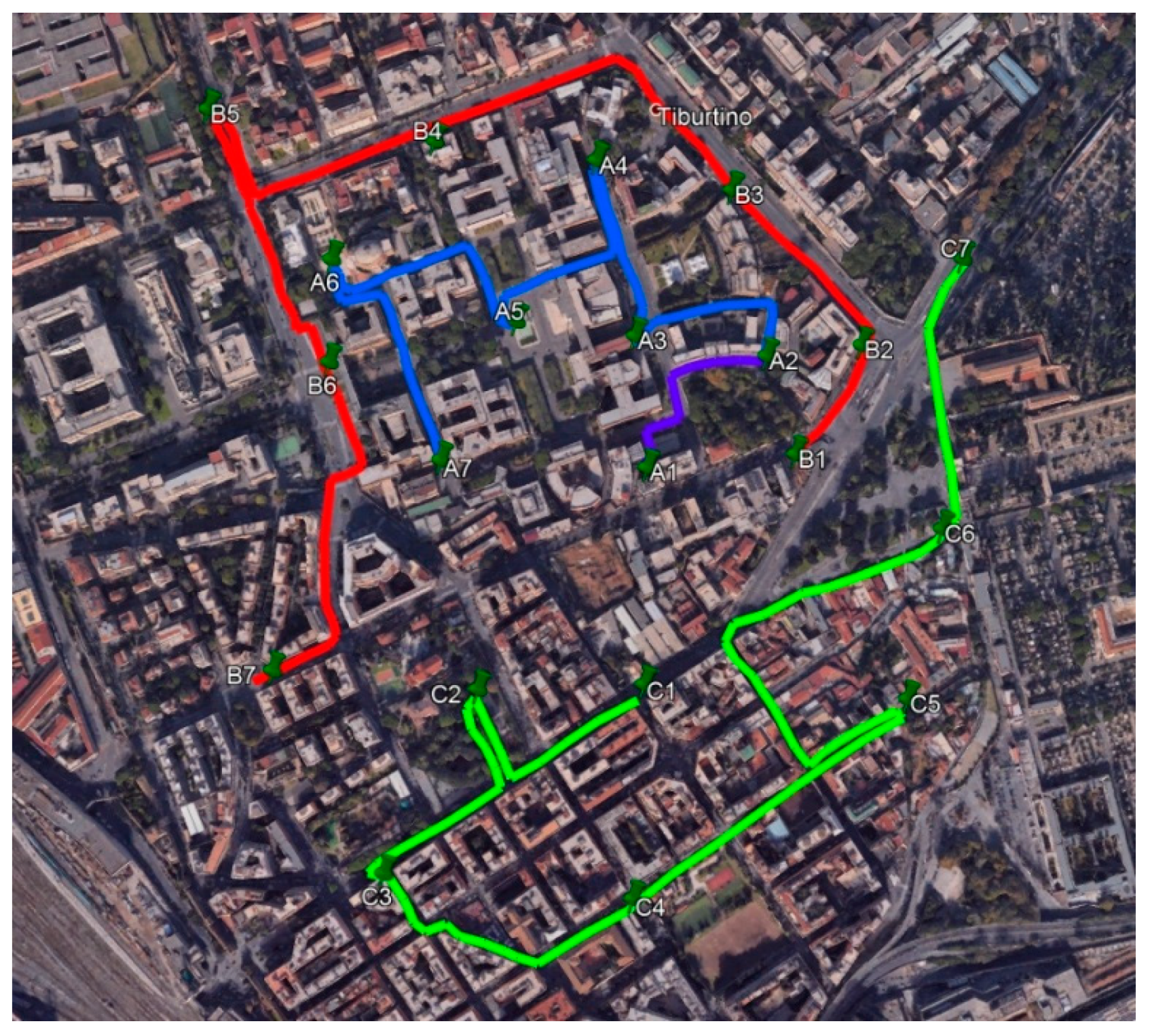
2.1. Study Domain and Monitoring Campaigns

The study domain has an area of 1 km² centered on the E. Fermi Physics building of Sapienza University, one of the largest and oldest universities in Europe, accounting for more than 100,000 students and about 8000 workers, in the district of San Lorenzo in Rome (Italy). The university campus extends over an area of 0.22 km² where parking is allowed to a limited number of cars.

The sampling points were chosen with the aim of obtaining the maximum spatial gradient. It was assumed from a previous study [11] that spatial variability mainly depends on the traffic on the main roads and on the building shape and density.

Moreover, the sampling points within the university were chosen considering the effects of buildings on the wind. For this reason, a series of preliminary simulations with high spatial resolution were carried out using the three-dimensional, non-hydrostatic ENVIMET numerical model, able to reproduce the fluid dynamic field in correspondence with groups of obstacles [52]. Four scenarios were simulated, corresponding to the four prevailing wind directions in the area under consideration [53], i.e., North (0°), Northeast (45°), South (180°), and Southwest (225°), with a constant wind intensity of 1.5 m/s (Supplementary Materials Figure S1). The reproduction of the prevailing anemological conditions allows the drawing of general conclusions not related to single events and, therefore, is particularly useful for the choice of sampling points.

In addition, the proximity to the surrounding nearest roads was taking into account.

PNC was measured using handheld condensation particle counters (CPC3007, TSI inc., Shoreview, MN) which operated at a flow of 100 mL/min measuring particles within the range of 10–1000 nm with a time resolution of 1 s. Due to the large amount of sampling points along with the limited number of available devices, a rounding measurement strategy was adopted. We selected three paths (Figure 1: A, blue line—inside the university, B, red line -all around the university fence, and C, green line—within the surrounding San Lorenzo district) with seven sampling points each; three operators carried out measurements contemporarily on each path. Each of the 21 selected measurement points was visited three times during the day at pre-established times, representing three specific time bands at local times 8:00–10:00; 12:00–14:00 and 16:00–18:00.

For each point, 10-min measurements were made. The CPCs were carried from an operator alongside the chosen path. Each sampling point was previously geolocated. Measurements were carried out by placing the CPC on top of a wood base mounted on a tripod (see Supplementary Materials Figure S2a–c).

Two monitoring campaigns were conducted on 8–17 November 2017 (cold season) and on 17–23 June 2018 (warm season) with the aim to capture the weekly and seasonal variability. Details on site-by-site descriptive statistics are reported in the Supplementary material (Tables S1 and S2).

The concentration data measured in 10 min in the November and June campaigns were reconstructed for an average time of two hours: two hours and ten minutes was in fact the time needed to visit the 7 sites of each path with measurements lasting 10 min, so the two-hour average was considered the average temporal unit of the models. The averaged values over the 2 h were reconstructed using continuous and parallel measurements carried out on the roof of the Physics building for the duration of the campaigns in June and November.

The two-hour mean PNC determined at the various points was used as the response variable of the model. In order to follow a normal distribution of the response variable (Figure 2), a logarithmic transformation was applied [34,54].

2.2. Potential Spatial Explanatory Variables

The calculated spatial variables were the following:

• Urban morphology: the volumes and heights of the buildings were obtained from the Urban Atlas 2012 section of the Copernicus Land Monitoring Service (https://land.copernicus.eu/local/urban-atlas/urban-atlas-2012; accessed on 16 November 2021), while the width and the length of the roads and the distance to them distinguishing among main, secondary and local ones, were evaluated starting from the Open Street Map layers (https://www.openstreetmap.org; accessed on 16 November 2021). Moreover, the urban morphology variables were used to calculate some parameters characterizing the urban canyon (see Supplementary Materials Figure S3).
• Land use: Urban green area, Continuous Urban Fabric representative of continuous areas with high population density, Discontinuity Density representative of discontinuous areas with medium-low population density and Industrial Commercial Public representative of public areas, were calculated in the domain of interest, starting from the data available in the Urban Atlas 2012 section of the Copernicus Monitoring Land Service, at spatial resolution of 10 m. Imperviousness, which was representative of impermeable surfaces, was calculated at a spatial resolution of 100 m.
• Population: the number of inhabitants was considered in the corresponding census sections, with reference to the last ISTAT census of 2011 (https://www.istat.it/it/archivio/104317; accessed on 16 November 2021).

Each spatial variable was calculated at the measurement points in buffers with a radius of 12.5 m and 25 m. GIS analyses and mapping were performed using ArcGIS (v.10.3; ESRI).

2.3. Potential Temporal Explanatory Variables—Meteorological Parameters

The time variables used as potential predictors were wind intensity and direction, air temperature, relative humidity, atmospheric pressure, height and intensity of rainfall and global solar radiation. Moreover, the standard deviation of wind intensity and turbulent kinetic energy (TKE) were taken into account since they are representative of the atmospheric turbulence [55].

The meteorological parameters were provided by the Regional Protection Agency of the Lazio (ARPA LAZIO). Measurements were carried out using a sonic anemometer placed on the roof of the ARPA LAZIO building located 2 km NW from the study domain center.

With the aim of providing information on the air dispersion volume, the planetary boundary layer height (PBLH) was estimated based on remote sensing measurements carried out using a Light Detection And Ranging (LiDAR) sensor belonging to the BAQUNIN supersite [56] and installed on the rooftop of the E. Fermi building, in the center of the domain. The measurements were carried out continuously during the summer measurement campaign, and the 10-min temporal resolution PBLH was retrieved following the procedure described in [57].

All time parameters were averaged over 2 h to be used in the empirical models.

2.4. Potential Spatial and Temporal Explanatory Variables—Traffic Flows

Traffic flows vary significantly both spatially and temporally.

Traffic data were based on traffic count taken during the measurement campaigns at each point (10-min cumulative counts); the average hourly traffic measured (vehicles/hour) was compared with the modelled traffic flows provided by the Mobility Agency of the Municipality of Rome, referring to an average year, in the main roads around the campus. Linear regression between the traffic measurements and estimations, for the monitoring campaigns in the three time bands in the cold season (8–12 November 2017) and the warm season (17–23 June 2018), were performed. The regression coefficients ranging between 0.62–0.79 in the cold season and 0.59–0.84 in the warm season. We then calculated, based on the regression equations, the traffic in the hours in which the traffic measurements were not carried out.

2.5. Models Development

The explanatory variables described were considered as potential predictors in the development of Generalized Additive Model (GAM, [34]). The GAM equation is defined as follows [40]:

$$\mathrm{g}\left({\mathsf{\mu }}_{\mathrm{i}}\right)={\mathrm{A}}_{\mathrm{i}}\mathsf{\gamma }+{{\displaystyle \sum }}_{\mathrm{j}}^{ }{\mathrm{f}}_{\mathrm{j}}\left({\mathrm{x}}_{\mathrm{ji}}\right), \mathrm{yi} ~ \mathrm{EF}({\mathsf{\mu }}_{\mathrm{i}}, \mathsf{\phi })$$

where:

yi = response variable

${\mathsf{\mu }}_{\mathrm{i}}$ ≡ E(yi) = expected value of yi

yi ~ EF(${\mathsf{\mu }}_{\mathrm{i}}$, φ) = exponential distribution of yi

${\mathrm{A}}_{\mathrm{i}}\mathsf{\gamma }$ = ith row of the model parameter matrix with its corresponding vector

${\mathrm{f}}_{\mathrm{j}}\left({\mathrm{x}}_{\mathrm{ji}}\right)$ = smoothing function for the covariates j

All the independent temporal variables in input to the model described above were attributed to the time average of two hours.

Three GAMs were fitted for the cold and warm week and for the overall period, using the log-transformed two-hour PNC averages as the response variable.

Among potential predictors only those with at least 90% non-zero data were selected. Correlation matrices for each group of variables (temporal, spatial and spatio-temporal) were presented in Table S3 and Figures S7–S9 of the Supplementary Materials; starting from the best correlation between these variables and the natural logarithm of PNC, a stepwise forward procedure was followed.

In the variable stepwise selection, each variable was added if: it gave an incremental R² adjusted higher than 1%; the a priori direction of the effect was respected and it did not change the direction of effect of previously added variables.

Moreover, test checks were performed to select the best spline for each variable. The smoothing parameter was chosen controlling the balance between likelihood function and the overfitting, founding the convergence of the iteration algorithm (gam check routine of the R mgcv package). The K (or K’ used in gam check routine) parameter represents the number of basis functions that determines how wiggly a smooth can be. Where not expressly indicated, it is assumed that the value of parameter K is equal to 10. The Effective Degrees of Freedom (EDF) represents the complexity of the smooth in terms of curve sinuosity (the higher the EDF value, the greater the spline non-linearity). If there are not enough basis functions, it may not be wiggly enough to capture the relationships in data (EDF is close to K’). The F parameter is used in an ANOVA test to confirm overall significance of the smooth.

Interactions between variables were also assessed using specific functions in the R mgcv package (e.g., “Tensor smooths”) [58].

Standardized data adaptation criteria, Akaike Information Criterion (AIC), Generalized Cross Validation (GCV) and Bayesian Information Criterion (BIC) were calculated for the developed models to control the phenomena of improper adaptation due to overfitting. Finally, residual normality was graphically checked in order to confirm the basic assumption.

Graphical tools and statistical indicators (k-fold Root Mean Square Error, k-fold CV, Adjusted R-Squared) were used to evaluate the performance of the GAMs fitted. The R software ([59,60] R Development Core Team) and in particular the gam function implemented in the mgcv library was used.

3. Results and Discussion

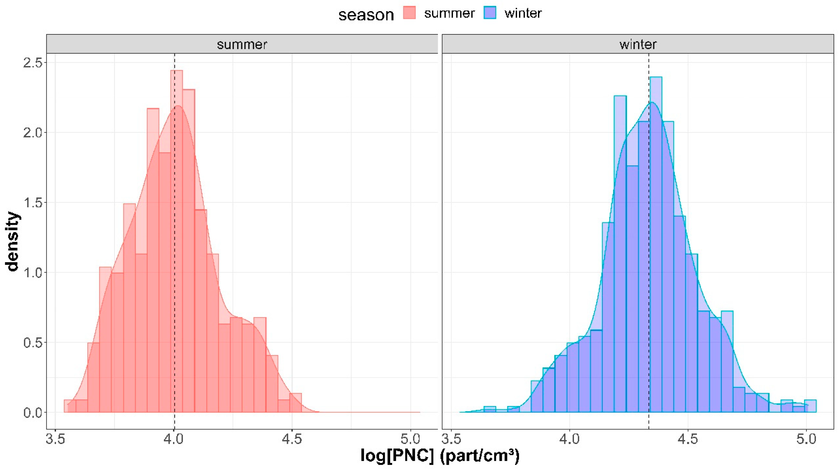
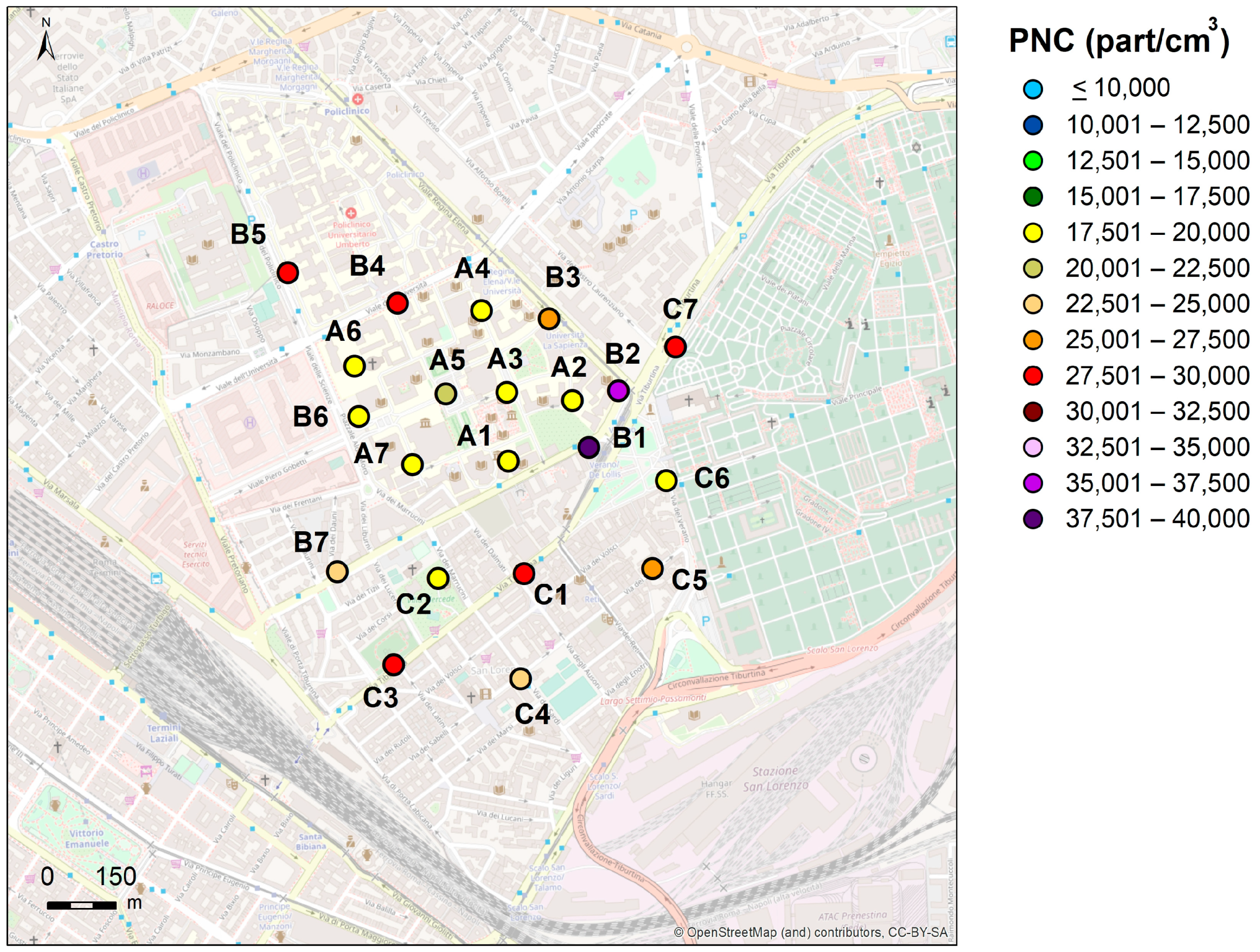
3.1. Particle Number Concentration Measurements

Figure 3 and Figure 4 show the point-by-point PNC weekly averages calculated during the first campaign (8–17 November 2017—cold season) and the second campaign (17–23 June 2018—warm season), respectively.

Two-hour averages PNC at measurement sites ranged between 3846 and 32,483 particles/cm³ in the warm season; the observed range was 5722–101,594 particles/cm³ during the cold season. The temporal variation, assessed by means of coefficient of variation calculated in each site, ranged between 27% and 71%. The within-area contrast (expressed as the estimated average concentration range by median ratios) was 91.7% and 86.4% in the cold and warm season, respectively. This addresses for the existence of a high spatial contrast in the PNC despite the small study domain, with implications on population exposure [5].

The cold season average values were approximately double that of the warm period (see Figure S4, for detailed site-by-site comparisons). Moreover, the PNC median was larger during working days than on Sundays (when traffic flows were reduced, see Figure S6). Saturday has intermediate concentration values between Sunday and the typical values of weekdays. These results confirmed that our monitoring strategy allows for sufficiently capturing the typical diurnal PNC variability (two rush hours maximum in the 8–10 and 16–18 time bands and the typical daily minimum in the 12–14 time band).

The seasonal and temporal variability observed were nicely in agreement with long-term PNC observations carried out within the same study domain at a traffic influenced site (located a few meters from the curbside [61,62], as well as with other studies across Europe e.g., [63]).

At the measurement points inside the university area (path A away from the roads), significantly lower values (p < 0.01) compared to those observed at the measurement spots along the two external paths, close to major roads with high traffic intensity (see B1, B2, B3, B4, B5, C1, C3 and C7) were observed. Conversely, the average concentrations at points B6, C2 and C6, relatively far from the high traffic roads, were comparable, in both seasons, with those within the university area.

These finding were consistent with the sampling point characterization showed in Figure S5, where the ratio between traffic flows on the nearest road and distance from the road traffic for each site was reported. With this regard, it should be noted that total traffic flows (calculated in directions AB + BA averaged over 2 h) were linearly correlated with PNC both in June (r = 0.48, p < 0.01) and in November (r = 0.39, p < 0.01).

The spatial contrast in measured PNC was represented by the ratio of the minimum and maximum value of the average two seasonal campaigns in the overall measurement points. The calculated parameter in overall 21 measurement points was 0.53 and was comparable with that estimated within the city of Rome (0.6) [11].

3.2. Model Evaluation

GAMs were performed to predict PNC in the study area for the cold and warm seasons (November 2017 and June 2018) and for the overall period (Overall model).

In the cold season model, the relative humidity (Urel), the traffic in the nearest street (Traff), the inverse distance squared to the nearest main/busy road (Distinv2), the difference between the maximum and minimum turbulent kinetic energy in two hours (DELTA_TKE) were selected as explanatory variables.

$$\ln \left(\mathrm{PNC}\right)= \mathrm{s}\left(\mathrm{Urel}\right)+\mathrm{s}\left(\mathrm{Distinv}2,\mathrm{k}=15\right)+\mathrm{s}\left(\mathrm{DELTA}\_\mathrm{TKE}\right)+\mathrm{Traff}$$

(1)

where:

Urel = Relative humidity (%)

Distinv2 = Inverse distance squared to the nearest road (1/m²)

DELTA TKE = Difference maximum turbulent kinetic energy and minimum turbulent kinetic energy (m²/s²)

Traff = Total traffic in directions AB + BA (vehicles/h)

The coefficient estimate and statistical significance are shown in

Table 1. Coefficients and significance of linear terms of the cold season model.

Variable [UM]	Coefficient (SE)	t Value	Pr (>|t|)
Intercept	9.90 (0.355)	278.8	<0.001
Traff [vehicles/h]	1.20 × 10−4 (5.22 × 10−5)	2.3	0.022

and

Table 2. Significance of smoothing terms of the cold season model.

Smoothing Terms [UM]	EDF	F	p Value	K’	k Index
s(Urel) [m−1]	8.342	33.705	<0.001	9.00	0.98
s(Distinv2, k = 15) [m−2]	12.293	7.379	<0.001	14.00	0.98
s(DELTA_TKE) [m2/s2]	8.975	19.283	<0.001	9.00	0.99

EDF (Effective Degrees of Freedom), F (parameter used in ANOVA test) and p-value were used to evaluate the significance of the smooth; K’ represented the number of basis function and k-index (ratio of neighbor differencing scale estimate to fitted model scale estimate) was used to evaluate the significance of the residuals.

.

In the summer model, the scalar wind speed (Vscal), the traffic in the nearest road (Traff), the inverse distance squared to the nearest main/busy road (Distinv2) and the height minimum of the PBL (Hmix_min) were selected as explanatory variables.

$$\ln \left(\mathrm{PNC}\right)= \mathrm{s}\left(\mathrm{Vscal}\right)+\mathrm{s}\left(\mathrm{Distinv}2,\mathrm{k}=12\right)+\mathrm{s}\left({\mathrm{Hmix}}_{\min }\right)+\mathrm{s}\left(\mathrm{Traff}\right)$$

where:

Vscal = average wind speed (m/s)

Distinv2 = Inverse distance squared to the nearest road (1/m²)

Hmix_min = minimum PBL height (m)

Traff = Total traffic in directions AB + BA (vehicles/h)

The coefficient estimate and statistical significance are shown in

Table 3. Coefficients and significance of linear terms of the warm season model.

Variable [UM]	Coefficients (SE)	t Value	Pr (>|t|)
Intercept	9.21 (0.011)	835	<0.001

and

Table 4. Significance of smoothing terms of the warm season model.

Smoothing Terms [UM]	EDF	F	p Value	K’	k Index
s(Vscal) [m/s]	9.000	10.087	<0.001	9.00	1.00
s(Distinv2, k = 12) [m−2]	9.728	15.370	<0.001	11.00	1.08
s(Hmixmin) [m]	6.504	21.105	<0.001	9.00	1.00
s(Traff) [vehicles/h]	3.561	2.577	0.029	9.00	1.08

EDF (Effective Degrees of Freedom), F (parameter used in ANOVA test) and p-value were used to evaluate the significance of the smooth; K’ represented the number of basis function and k-index (ratio of neighbor differencing scale estimate to fitted model scale estimate) was used to evaluate the significance of the residuals.

.

In the overall model, built using data for both periods together, the temperature (Tdry), the scalar wind speed (Vscal), the traffic in the nearest road (Traff), the inverse distance squared to the main/busy road (Distinv2), the difference between the maximum and minimum turbulent kinetic energy in 2 h (DELTA_TKE), were selected as explanatory variables.

$$\ln \left(\mathrm{PNC}\right)= \mathrm{s}\left(\mathrm{Tdry},\mathrm{k}=15\right)+\mathrm{s}\left(\mathrm{Distinv}2,\mathrm{k}=12\right)+\mathrm{s}\left(\mathrm{Vscal},\mathrm{k}=15\right)+\mathrm{s}\left(\mathrm{DELTA}\_\mathrm{TKE},\mathrm{k}=15\right)+\mathrm{Traff}$$

where:

Tdry = Temperature (°C)

Distinv2 = Inverse distance squared to the nearest road (1/m²)

Vscal = average wind speed (m/s)

DELTA_TKE = Difference maximum turbulent kinetic energy and minimum turbulent kinetic energy (m²/s²)

Traff = Total traffic in directions AB + BA (vehicles/h)

The coefficient estimate and statistical significance are shown in

Table 5. Coefficients and significance of linear terms of the overall model.

Variable [UM]	Coefficients (SE)	t Value	Pr (>|t|)
Intercept	9.57 (0.022)	436	<0.001
Traff [vehicles/h]	6.86 × 10−5 (2.45 × 10−5)	2.80	0.005

and

Table 6. Significance of smoothing terms of the overall model.

Smoothing Terms [UM]	EDF	F	p Value	K’	k Index
s(Tdry, k = 15) [°C]	12.29	79.04	<0.001	14.0	1.04
s(Distinv2, k = 12) [m−2]	10.74	23.24	<0.001	11.0	0.98
s(Vscal) [m/s]	13.89	17.81	<0.001	14.0	1.04
s(DELTA_TKE) [m2/s2]	13.45	15.00	<0.001	14.0	1.04

EDF (Effective Degrees of Freedom), F (parameter used in ANOVA test) and p-value were used to evaluate the significance of the smooth; K’ represented the number of basis function, and k-index (ratio of neighbor differencing scale estimate to fitted model scale estimate) was used to evaluate the significance of the residuals.

.

The smooth terms for the three models (Table 1, Table 2, Table 3, Table 4, Table 5 and Table 6) are all significant (p-value < 0.001), and the choices of the K parameter for each variable return satisfactory results (k index > 1).

As shown in Figures S11, S13 and S15, for the three models the basic assumptions were respected: residuals were normally distributed and the constancy of variance, and independence of the variables were respected in accordance with the random distribution of the residuals versus estimated values.

3.3. Models Performance

The performance indices for the three models are shown in

Table 7. Performance parameters of the three GAMs.

Model	R2 adj	R2	GCV	AIC	BIC	RMSE [part/cm3]
Cold season	0.690	71.1%	0.073	93.95	227,3	7743
Warm season	0.779	79.7%	0.047	−76.2	43.558	2832
Overall	0.835	84.5%	0.06	13.482	278.646	5562

. In particular, a very good space-time prediction index is represented by the Root Mean Square Error (RMSE). K-fold cross-validation has been used to estimate the prediction error [64].

The cold season model explains 71.1% of the deviance (adjusted R² equal to 0.690). The summer model explains 79.7% of the deviance (adjusted R² equal to 0.779). The overall model explains 84% of the deviance (adjusted R² equal to 0.835). RMSE of the models showed rather satisfactory values. All performance parameters were consistent with those of other previous studies [34,35].

3.4. Influence of Explanatory Variables

To assess the influence of explanatory variables on estimated PNC levels, the percent relative effect (P) of each variable was calculated through the following equation [65,66]:

P = (e^α − 1) × 100%

where:

α = ln (variable effect)

P can be interpreted as PNC percentage change in relation to the baseline level.

The frequency ratio of negative relative effect by meteorological covariate (NR) was calculated to better understand the sign of relative contributions, regardless of the magnitude. For each covariate NR parameter was calculated by the following equation:

NR = Nneg/Npos

where:

-

Nneg = n. of occurrences with negative p value

-

Npos = n. of occurrences with positive p value

NR and the P median values, also disaggregated by time bands, are shown in

Table 8. Influence of variables on estimated PNC levels in the three models.

Cold Season Model
	s(Urel)	s(DELTA_TKE)		Traff	s(Distnv2)
Median relative effect	−15.3%	18.2%		6.65%	1.84%
NR	1.3	0.4		0.0	0.9
Warm season model
	s(Vscal)	s(Hmixmin)		s(Traff)	s(Distnv2)
Median relative effect	−27.6%	45.8%		1.46%	−7.69%
NR	2.4	0.4		0.8	1.1
Overall model
	s(Tdry)	s(DELTA_TKE)	s(Vscal)	Traff	s(Distnv2)
Median relative effect	−0.74%	−3.35%	−7.10%	3.38%	−1.19%
NR	1.0	2.0	1.1	0.0	1.1

and

Table 9. Influence of variables (median relative effect) on estimated PNC levels in the three models and in the three specific time bands.

Cold Season Model
Time bands	s(Urel)	s(DELTA_TKE)		Traff	s(Distnv2)
8	12.0%	22.9%		4.27%	1.84%
12	−20.5	11.5%		8.67%	1.84%
16	−19.4%	23.4%		7.79%	1.84%
Warm season model
Time bands	s(Vscal)	s(Hmixmin)		s(Traff)	s(Distnv2)
8	−23.1%	49.1%		0.55%	−7.69%
12	−21.6%	−2.03%		1.85%	−7.69%
16	−44.8%	45.8%		1.84%	−7.69%
Overall model
Time bands	s(Vscal)	s(Tdry)	s(DELTA_TKE)	Traff	s(Distnv2)
8	43.3%	19.7%	−18.2%	2.55%	−1.19%
12	−16.4%	−28.9%	−1.63%	4.08%	−1.19%
16	−11.2%	−15.1%	−2.04%	3.90%	−1.19%

.

In the summer model, Hmix_min had the greatest percent relative effect, causing an increase in PNC of 45.8%, whereas Vscal exhibited a relevant negative effect (p = −27.6%). Meteorology variables proved to have a strong effect in the winter season too, even if smaller than the summer one: the biggest contribution to PNC increase (p = 18.2%) was caused by DELTA_TKE, while that to PNC decrease was due to Urel (p = −15.3%). The overall model results confirmed the significant effect of meteorological parameters.

Both Vscal and Urel had prevalence of negative effect occurrences. Hmix_min showed a strong positive effect frequency. DELTA_TKE exhibited a large prevalence of negative effect occurrences in the overall model, instead a relevant prevalence of positive effect in the winter one.

Looking at the overall model in Table 9, for all variables (with the exception of DELTA_TKE), the smallest percentage contribution increase took place during the evening band. In the winter model, Urel exhibited a strong negative contribution during the noontime and evening bands. In the summer model, Vscal showed a great negative effect, especially in the evening. Traffic flow contribution during the winter period resulted bigger than in summer, and during the noontime band achieved a not-negligible 8.67% relative effect.

Discussion on Influence of Meteorological Parameters

The results of the cold season model showed a negative contribution of Urel (−15.3% in Table 8) while the trend of spline function (Figure S10) was consistent with the studies that showed an increase of PNC at low temperatures and high humidity, due to the phenomena of new particles’ formation [29,67]. Vehicle emissions consist of a mixture of hot organic gases and sulfur and nitrogen oxides, together with particles. The mixture of hot gases meets cold air, rapidly forming ultrafine particles in the nucleation mode (1–20 nm) in the first seconds after emission [32,68]. These particles are always formed, but their formation is favored by low temperature and high humidity and have been observed in traffic sites near the sources [25,69].

DELTA_TKE variable was a good interpreter of the standard deviation of the horizontal wind speed [70]. DELTA_TKE showed a different contribution during the cold season and the overall models (18.2% and −3.35%, respectively, see Table 8). The relationship with PNC was positive in the range 0.0–1.0 m²/s² (Figures S10 and S14) that was also the range that reproduce very well the daily temporal variability in the overall monitoring periods. Measured values in the chosen time slot (black dots in Figure 5a,b) seem well distributed related to daily variability in the overall period (continuous red line): out of that range, DELTA_TKE variable exhibited explanatory weakness as confirmed by confidence intervals of the spline functions.

Traffic flow contribution was positive with PNC in all the three models, although a greater contribution was evident in the winter period compared to the summer one. It is well known that the new particles’ formation phenomena in the atmosphere by nucleation related to photochemical processes can be relevant in the summer period (the so-called midday nucleation events [18,71]), but particles formed through such events have been reported to fall mainly in the range 3–10 nm, which is outside the counting efficiency of the instruments we used.

Vscal had an important negative contribution in the warm season model, and less in the overall model (−27.6%, −7.10% in Table 8), in line with the trend of spline functions (Figures S12 and S14) that, with the limit of interval confidence, was consistent with several studies that showed a decrease of UFP with an increase of wind speed [25,34]; a decreasing exponential function was proposed with the minimum observed during a wind speed higher than 5 m/s [72]. In our study, the wind speed during summer (averaged over two hour) ranged between 1.0 and 2.9 m/s, and the spline has a maximum at around 2.0 m/s. However, it can be argued that, when the wind speed increases, the availability of particles on which the gases can condense is reduced, and therefore the probability that these lead to the formation of new particles increases (this also explains why in rural sites, where the concentration of particles is lower, the phenomena of formation of new particles have been shown to be more intense) [73].

The temporal variability is strongly dependent on the PBLH evolution over time and on the characteristics of the local wind. The trend of spline function of Hmix_min (Figure S12) showed a relationship with PNC that was consistent with what we generally expect in summer: the higher the atmospheric vertical turbulence, the lower the PNC as the other pollutants’ concentration [25,74]. A typical summer trend in the aerosol vertical profile and PBLH was showed in Figure 6 and Figure 7. The PBLH tends to increase with the increase in solar radiation, which favors convective phenomena until it reaches a maximum in the hottest hours of the day and then falls again in the afternoon.

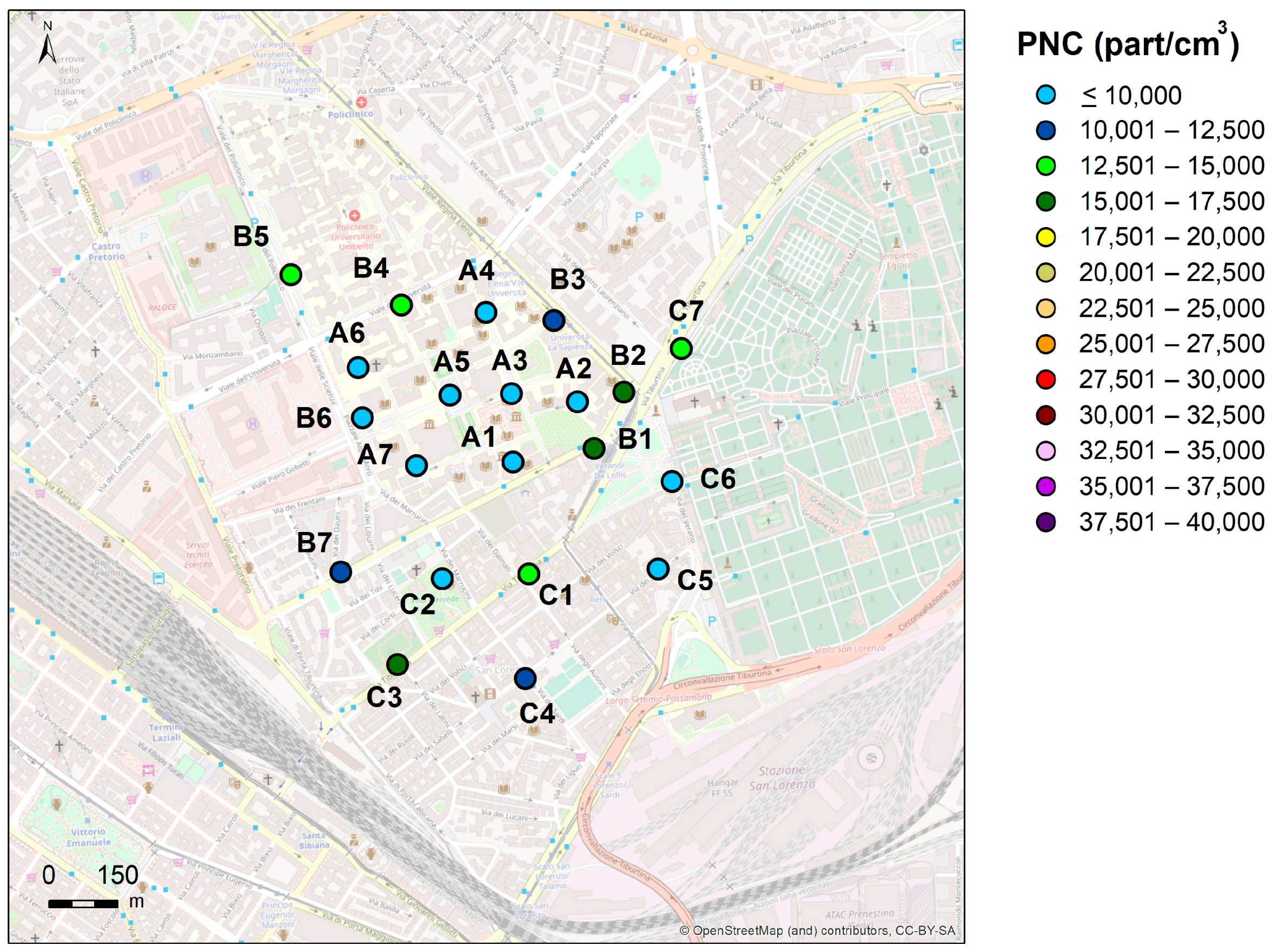
3.5. Spatio-Temporal Predictions of PNC

Variables selected for each model were calculated at each study domain cell (25 m × 25 m). The models’ equations were used to estimate average of PNCs at a two-hour time resolution. Inverse distance weighted interpolation of the resulting gridded PNCs was then used to generate PNC maps.

Figure 8, Figure 9 and Figure 10 show the spatial and temporal estimates of PNC in the study domain for a typically summer day, Wednesday 20 June 2018, in the three-time bands 8:00–10:00; 10:00–12:00 and 16:00–18:00.

The maps show the model capability to capture the intra-day PNC variability. The PBLH temporal trend and the traffic flow pattern drive the PNC spatiotemporal variability, since both traffic related variables and PBLH were important predictors in the warm season model.

PBLH tends to gradually increase in the morning until it reaches very high values, which remain stable from 1 pm to about 7 pm (on average 2500 m—as shown in Figure 7). The estimated PNC were high in the morning (low PBL and high traffic values—Figure 8) continue to increase up to 12 (still low PBL—Figure 9) until they decrease over the entire domain due to the phenomena of dispersion (high PBL—Figure 10).

Maximum PNC levels were found along the busiest streets, while large PNC decline was observed just a few tens of meters away from the curbside.

4. Conclusions

We developed GAMs to predict both spatially and temporally resolved PNC variability at a local (neighborhoods) scale.

The modeling approach effectiveness was demonstrated quantitatively.

All the three models were fully compliant with the basic assumptions for the GAM models, as demonstrated by diagnostic GAM plot [34,35].

The stepwise procedure allows for developing generally robust models which perform reasonably well in the cross-validation approach: the R² adjusted (0.690–0.835) was higher or within the range of the best performing statistical models already developed at the urban scale [34,41] and local scale [17,35].

Considering that the relationships between the target variable (PNC) and the potential predictors were not linear, we demonstrated that including spline functions with small uncertainty levels significantly improved the models’ performance (LUR R²_adj = 0.528 vs. GAM R²_adj = 0.835).

To the best of the authors’ knowledge, there are few studies [12,50] that have addressed the challenge to capture and effectively represent UFP urban hotspots spatial variability, at a local or microscale, through statistical models. Among them, ours is the only one accounting for seasonal and diurnal variability, although the temporal distribution was only suitable within the limit of the measurement ranges of the descriptive variables of the models.

The PNC variability main descriptors and their contribution to the PNC-explained variance were assessed. Based on our best knowledge, this study was the first that demonstrated the usefulness of time-resolved traffic counts to predict both spatial and temporal PNCs while accounting for traffic load as well as meteorology, allowing for reliable spatio-temporal predictions of PNC. In particular, the influence of atmospheric parameters showed that, in the summer model, there was the greatest percent relative effect of a single meteorological variable (Hmix_min), whereas in the winter season and overall models the effects of meteorological parameters were generally comparable.

As far as we know, a few numerical simulations have been developed to predict PNC at a street/local scale [18,75,76,77]; however, reliable emission inventories as well as monitoring networks for the models’ validation are still sparse [76,77,78,79]. Thus, statistical models remain to date a reliable and computationally affordable way to address the challenge.

In this study, our attention was focused on an area where the main activities take place, on the Sapienza university. It is one of the largest and oldest universities in Europe and has more than 100,000 students and about 8000 workers.

From the point of view of exposure, it therefore represents a rather large population with unique characteristics in terms of age distribution (mainly young adults) and prevailing health status.

We have highlighted that there is a significant difference between the concentrations detected in the internal areas of the university campus and those detected in the immediately adjacent external areas. In the former, students and university staff spend a large part of their day studying or working, but in the latter, they spend a significant part of their day for recreational and leisure activities (given the presence of a dense network of clubs, pubs, bars and restaurants that welcome them during breaks and in the evening).

However, also in the areas outside the university campus there is a significant variability essentially linked to the distance from the main traffic arteries. This variability affects the student, worker and resident population in the area itself.

A significant difference was also observed in the average summer levels (lower) compared to the winter ones, even if the spatial variability in the two seasons remains almost unchanged. This aspect is also important considering that the level of attendance of the campus in the two seasons is very different [80].

The method to assess PNC temporal and spatial variability proposed in this study can therefore represent a useful tool for the development of future studies that aim to estimate the integrated daily residential exposure to ultrafine particles of people that live, work or study in the area.

Moreover, our monitoring and modelling strategy could be easily replicable, with little economic effort, in other contexts as well as whenever monitoring data are needed to validate numerical simulations.

References

1. Schraufnagel, D.E. The health effects of ultrafine particles. Exp. Mol. Med. 2020, 52, 311–317. [Google Scholar] [CrossRef] [PubMed]
2. Hong, G.; Jee, Y.-K. Special issue on ultrafine particles: Where are they from and how do they affect us? Exp. Mol. Med. 2020, 52, 309–310. [Google Scholar] [CrossRef]
3. Stafoggia, M.; Schneider, A.; Cyrys, J.; Samoli, E.; Andersen, Z.J.; Bedada, G.B.; Bellander, T.; Cattani, G.; Eleftheriadis, K.; Faustini, A.; et al. Association between Short-Term Exposure to Ultrafine Particles and Mortality in Eight European Urban Areas. Epidemiology 2017, 28, 172–180. [Google Scholar] [CrossRef] [PubMed]
4. Samoli, E.; Andersen, Z.J.; Katsouyanni, K.; Hennig, F.; Kuhlbusch, T.A.J.; Bellander, T.; Cattani, G.; Cyrys, J.; Forastiere, F.; Jacquemin, B.; et al. Exposure to ultrafine particles and respiratory hospitalisations in five European cities. Eur. Respir. J. 2016, 48, 674–682. [Google Scholar] [CrossRef] [PubMed]
5. Belleudi, V.; Faustini, A.; Stafoggia, M.; Cattani, G.; Marconi, A.; Perucci, C.A.; Forastiere, F. Impact of fine and ultrafine particles on emergency hospital admissions for cardiac and respiratory diseases. Epidemiology 2010, 21, 414–423. [Google Scholar] [CrossRef] [PubMed]
6. Hoek, G.; Beelen, R.; Kos, G.; Dijkema, M.; van der Zee, S.C.; Fischer, P.H.; Brunekreef, B. Land use regression model for ultrafine particles in Amsterdam. Environ. Sci. Technol. 2011, 45, 622–628. [Google Scholar] [CrossRef] [PubMed]
7. Abernethy, R.C.; Allen, R.W.; McKendry, I.G.; Brauer, M. A land use regression model for ultrafine particles in Vancouver, Canada. Environ. Sci. Technol. 2013, 47, 5217–5225. [Google Scholar] [CrossRef] [PubMed] [Green Version]
8. Saraswat, A.; Apte, J.S.; Kandlikar, M.; Brauer, M.; Henderson, S.B.; Marshall, J.D. Spatiotemporal land use regression models of fine, ultrafine, and black carbon particulate matter in New Delhi, India. Environ. Sci. Technol. 2013, 47, 12903–12911. [Google Scholar] [CrossRef]
9. Patton, A.P.; Zamore, W.; Naumova, E.N.; Levy, J.I.; Brugge, D.; Durant, J.L. Transferability and Generalizability of Regression Models of Ultrafine Particles in Urban Neighborhoods in the Boston Area. Environ. Sci. Technol. 2015, 49, 6051–6060. [Google Scholar] [CrossRef] [PubMed] [Green Version]
10. Sabaliauskas, K.; Jeong, C.; Yao, X.; Reali, C.; Sun, T.; Evans, G.J. Development of a land-use regression model for ultrafine particles in Toronto, Canada. Atmos. Environ. 2015, 110, 84–92. [Google Scholar] [CrossRef]
11. Cattani, G.; Gaeta, A.; Di Menno di Bucchianico, A.; De Santis, A.; Gaddi, R.; Cusano, M.; Ancona, C.; Badaloni, C.; Forastiere, F.; Gariazzo, C.; et al. Development of land-use regression models for exposure assessment to ultrafine particles in Rome, Italy. Atmos. Environ. 2017, 156, 52–60. [Google Scholar] [CrossRef]
12. Ghassoun, Y.; Löwner, M.-O. Land use regression models for total particle number concentrations using 2D, 3D and semantic parameters. Atmos. Environ. 2017, 166, 362–373. [Google Scholar] [CrossRef]
13. Yang, Z.; Freni-Sterrantino, A.; Fuller, G.W.; Gulliver, J. Development and transferability of ultrafine particle land use regression models in London. Sci. Total Environ. 2020, 740, 140059. [Google Scholar] [CrossRef]
14. Olvera, H.A.; Jimenez, O.; Provencio-Vasquez, E. Modeling particle number concentrations along Interstate 10 in El Paso, Texas. Atmos. Environ. 2014, 98, 581–590. [Google Scholar] [CrossRef] [Green Version]
15. Rivera, M.; Basagaña, X.; Aguilera, I.; Agis, D.; Bouso, L.; Foraster, M.; Medina-Ramón, M.; Pey, J.; Künzli, N.; Hoek, G. Spatial distribution of ultrafine particles in urban settings: A land use regression model. Atmos. Environ. 2012, 54, 657–666. [Google Scholar] [CrossRef]
16. Eeftens, M.; Meier, R.; Schindler, C.; Aguilera, I.; Phuleria, H.; Ineichen, A.; Davey, M.; Ducret-Stich, R.; Keidel, D.; Probst-Hensch, N.; et al. Development of land use regression models for nitrogen dioxide, ultrafine particles, lung deposited surface area, and four other markers of particulate matter pollution in the Swiss SAPALDIA regions. Environ. Health 2016, 15, 53. [Google Scholar] [CrossRef] [PubMed] [Green Version]
17. Kerckhoffs, J.; Hoek, G.; Gehring, U.; Vermeulen, R. Modelling nationwide spatial variation of ultrafine particles based on mobile monitoring. Environ. Int. 2021, 154, 106569. [Google Scholar] [CrossRef] [PubMed]
18. Zhang, K.M.; Wexler, A.S.; Zhu, Y.F.; Hinds, W.C.; Sioutas, C. Evolution of particle number distribution near roadways. Part II: The ′Road-to-Ambient′ process. Atmos. Environ. 2004, 38, 6655–6665. [Google Scholar] [CrossRef]
19. Sioutas, C.; Ralph, J.; Delfino, R.J.; Manisha, S. Exposure assessment for atmospheric ultrafine particles (UFPs) and implications in epidemiologic research. Environ. Health Perspect. 2005, 113, 947–955. [Google Scholar] [CrossRef] [PubMed] [Green Version]
20. Zhou, Y.; Levy, I.J. Factors influencing the spatial extent of mobile source air pollution impacts: A meta-analysis. BMC Public Health 2007, 7, 89. [Google Scholar] [CrossRef] [PubMed] [Green Version]
21. Ketzel, M.; Berkowicz, R. Modelling the fate of ultrafine particles from exhaust pipe to rural background: An analysis of time scales for dilution, coagulation and deposition. Atmos. Environ. 2004, 38, 2639–2652. [Google Scholar] [CrossRef]
22. Kittelson, D.B.; Watts, W.F.; Johnson, J.P. Nanoparticle emissions on Minnesota highways. Atmos. Environ. 2004, 38, 9–19. [Google Scholar] [CrossRef]
23. Zhu, Y.; Hindsa, W.C.; Kim, S.; Shen, S.; Sioutas, C. Study of ultrafine particles near a major highway with heavy-duty diesel traffic. Atmos. Environ. 2002, 36, 4323–4335. [Google Scholar] [CrossRef]
24. Fujitani, Y.; Kumar, P.; Tamura, K.; Fushimi, A.; Hasegawa, S.; Takahashi, K. Seasonal differences of the atmospheric particle size distribution in a metropolitan area in Japan. Sci. Total Environ. 2012, 437, 339–347. [Google Scholar] [CrossRef] [Green Version]
25. Morawska, L.; Ristovski, Z.; Jayaratne, E.R.; Keogh, D.U.; Ling, X. Ambient nano and ultrafine particles from motor vehicle emissions: Characteristics, ambient processing and implications on human exposure. Atmos. Environ. 2008, 42, 8113–8138. [Google Scholar] [CrossRef] [Green Version]
26. Kumar, P.; Robins, A.; Vardoulakis, S.; Britter, R. A review of the characteristics of nanoparticles in the urban atmosphere and the prospects for developing regulatory controls. Atmos. Environ. 2010, 44, 5035–5042. [Google Scholar] [CrossRef] [Green Version]
27. Kulmala, M.; Vehkamaki, H.; Petaja, T.; Dal Maso, M.; Lauri, A.; Kerminen, V.; Birmilli, W.; McMurry, P. Formation and growth rates of ultrafine atmospheric particles: A review of observations. J. Aerosol Sci. 2004, 35, 143–176. [Google Scholar] [CrossRef]
28. Holmes, N. A review of particle formation events and growth in the atmosphere in the various environments and discussion of mechanistic implications. Atmos. Environ. 2007, 41, 2183–2201. [Google Scholar] [CrossRef] [Green Version]
29. Raes, F.; Dingenen, R.V.; Vignati, E.; Wilson, J.; Putaud, J.-P.; Seinfeld, J.H.; Adams, P. Formation and cycling of aerosols in the global troposphere. Atmos. Environ. 2000, 34, 4215–4240. [Google Scholar] [CrossRef]
30. Birmili, W.; Wiedensohler, A. New particle formation in the continental boundary layer: Meteorological and gas phase parameter influence. Geophys. Res. Lett. 2000, 27, 3325–3328. [Google Scholar] [CrossRef]
31. Boy, M.; Kulmala, M. Nucleation events in the continental boundary layer: Influence of physical and meteorological parameters. Atmos. Chem. Phys. 2002, 2, 1–16. [Google Scholar] [CrossRef] [Green Version]
32. Ma, N.; Birmili, W. Estimating the contribution of photochemical particle formation to ultrafine particle number averages in an urban atmosphere. Sci. Total Environ. 2015, 512–513, 154–166. [Google Scholar] [CrossRef] [Green Version]
33. Salvador, P.; Barreiro, M.; Gómez-Moreno, F.J.; Alonso-Blanco, E.; Artíñano, B. Synoptic classification of meteorological patterns and their impact on air pollution episodes and new particle formation processes in a south European air basin. Atmos. Environ. 2021, 245, 118016. [Google Scholar] [CrossRef]
34. Clifford, S.; Choy, S.L.; Hussein, T.; Mengersen, K.; Morawska, L. Using the Generalised Additive Model to model the particle number count of ultrafine particles. Atmos. Environ. 2011, 45, 5934–5945. [Google Scholar] [CrossRef]
35. Sartini, C.; Sajani, S.Z.; Ricciardelli, I.; Delgado-Saborit, J.M.; Scotto, F.; Trentini, A.; Ferrari, S.; Poluzzi, V. Ultrafine particle concentrations in the surroundings of an urban area: Comparing downwind to upwind conditions using Generalized Additive Models (GAMs). Environ. Sci. Processes Impacts 2013, 15, 2087–2095. [Google Scholar] [CrossRef] [PubMed]
36. Hastie, T.; Tibshirani, R. Generalized Additive Models; Chapman and Hall: New York, NY, USA, 1990. [Google Scholar]
37. Hussein, T.; Karppinen, A.; Kukkonen, J.; Härkönen, J.; Aalto, P.P.; Hämeri, K.; Kerminen, V.-M.; Kulmala, M. Meteorological dependence of sizefractionated number concentrations of urban aerosol particles. Atmos. Environ. 2006, 40, 1427–1440. [Google Scholar] [CrossRef]
38. Zuur, A.F.; Ieno, E.N.; Walker, N.; Saveliev, A.A.; Smith, G.M. Mixed Effects Models and Extensions in Ecology with R; Springer: Berlin, Germany, 2009; ISBN 978-0-387-87457-9. [Google Scholar]
39. Zuur, A.F. Beginner′s Guide to Generalized Additive Models with R; Highland Statistics Ltd.: Newburgh, UK, 2012; ISBN 978-0-957-17412-2. [Google Scholar]
40. Wood, S.N. Generalized Additive Models: An Introduction with R, 2nd ed.; Chapman and Hall/CRC: Boca Raton, FL, USA, 2017; ISBN 978-1-4987-2833-1. [Google Scholar]
41. Gerling, L.; Löschau, G.; Wiedensohler, A.; Weber, S. Statistical modelling of roadside and urban background ultrafine and accumulation mode particle number concentrations using generalized additive models. Sci. Total Environ. 2020, 703, 134570. [Google Scholar] [CrossRef]
42. Weissert, L.F.; Salmond, J.A.; Miskell, G.; Alavi-Shoshtari, M.; Wiliams, D.E. Development of a microscale land use regression model for predicting NO2 concentrations at a heavy trafficked suburban area in Auckland, NZ. Sci. Total Environ. 2018, 619–620, 112–119. [Google Scholar] [CrossRef]
43. Eeftens, M.; Beekhuizen, J.; Beelen, R.; Wang, M.; Vermeulen, R.; Brunekreef, B.; Huss, A.; Hoek, G. Quantifying urban street configuration for improvements in air pollution models. Atmos. Environ. 2013, 72, 1–9. [Google Scholar] [CrossRef]
44. Miskell, G.; Salmond, J.; Longley, I.; Dirks, K.N. A novel approach in quantifying the effect of urban design features on local-scale air pollution in central urban areas. Environ. Sci. Technol. 2015, 49, 9004–9011. [Google Scholar] [CrossRef]
45. Vardoulakis, S.; Solazzo, E.; Lumbreras, J. Intra-urban and street scale variability of BTEX, NO2 and O3 in Birmingham, UK: Implications for exposure assessment. Atmos. Environ. 2011, 45, 5069–5078. [Google Scholar] [CrossRef]
46. Grange, S.K.; Dirks, K.N.; Costello, S.B.; Salmond, J.A. Cycleways and footpaths: What separation is needed for equivalent air pollution dose between travel modes? Transp. Res. Part D Transp. Environ. 2014, 32, 111–119. [Google Scholar] [CrossRef]
47. Salmond, J.A.; McKendry, I.G. Influences of Meteorology on Air Pollution Concentrations and Processes in Urban Areas. In Air Quality in Urban Environment; Royal Society of Chemistry: London, UK, 2009; pp. 23–41. [Google Scholar]
48. Salmond, J.A.; Williams, D.E.; Laing, G.; Kingham, S.; Dirks, K.; Longley, I.; Henshaw, G.S. The influence of vegetation on the horizontal and vertical distribution of pollutants in a street canyon. Sci. Total Environ. 2013, 443, 287–298. [Google Scholar] [CrossRef] [PubMed]
49. Shi, Y.; Lau, K.K.; Ng, E. Developing street-level PM2.5 and PM10 land use regression models in high-density Hong Kong with urban morphological factors. Environ. Sci. Technol. 2016, 50, 8178–8187. [Google Scholar] [CrossRef] [PubMed]
50. Lin, M.Y.; Guo, Y.X.; Chen, Y.C.; Chen, W.T.; Young, L.H.; Lee, K.J.; Wu, Z.Y.; Tsai, P.J. An instantaneous spatiotemporal model for predicting traffic-related ultrafine particle concentration through mobile noise measurements. Sci. Total Environ. 2018, 636, 1139–1148. [Google Scholar] [CrossRef]
51. Pelliccioni, A.; Monti, P.; Cattani, G.; Boccuni, F.; Cacciani, M.; Canepari, S.; Capone, P.; Catrambone, M.; Cusano, M.; D′Ovidio, M.C.; et al. Integrated Evaluation of Indoor Particulate Exposure: The VIEPI Project. Sustainability 2020, 12, 9758. [Google Scholar] [CrossRef]
52. Bruse, M.; Fleer, H. Simulating surface–plant–air interactions inside urban environments with a three-dimensional numerical model. Environ. Model. Softw. 1998, 13, 373–384. [Google Scholar] [CrossRef]
53. Di Bernardino, A.; Iannarelli, A.M.; Casadio, S.; Mevi, G.; Campanelli, M.; Casasanta, G.; Cacciani, M. On the effect of sea breeze regime on aerosols and gases properties in the urban area of Rome, Italy. Urban Clim. 2021, 37, 100842. [Google Scholar] [CrossRef]
54. Patton, A.P.; Collins, C.; Naumova, E.N.; Zamore, W.; Brugge, D.; Durant, J.L. An hourly regression model for ultrafine particles in a near-highway urban area. Environ. Sci. Technol. 2014, 48, 3272–3280. [Google Scholar] [CrossRef] [Green Version]
55. Wyngard, J.C. Turbulence in the atmosphere. Bound.–Layer Meteorol. 2011, 139, 543–549. [Google Scholar]
56. Iannarelli, A.M.; Di Bernardino, A.; Casadio, S.; Bassani, C.; Cacciani, M.; Campanelli, M.; Casasanta, G.; Cadau, E.; Diémoz, H.; Mevi, G.; et al. The Boundary-Layer Air Quality-Analysis Using Network of INstruments (BAQUNIN) Supersite for Atmospheric Research and Satellite Validation over Rome Area. Bull. Am. Meteorol. Soc. 2021, under review.
57. Pichelli, E.; Ferretti, R.; Cacciani, M.; Siani, A.M.; Ciardini, V.; Di Iorio, T. The role of urban boundary layer investigated with high-resolution models and ground-based observations in Rome area: A step towards understanding parameterization potentialities. Atmos. Meas. Tech. 2014, 7, 315–332. [Google Scholar] [CrossRef] [Green Version]
58. Wood, S. Mixed GAM Computation Vehicle with Automatic Smoothness Estimation. 2019. Available online: https://cran.r-project.org/web/packages/mgcv/mgcv.pdf (accessed on 16 November 2021).
59. R Core Team. R: A Language and Environment for Statistical Computing; R Foundation for Statistical Computing: Vienna, Austria, 2020; Available online: https://www.R-project.org/ (accessed on 16 November 2021).
60. RStudio Team. RStudio: Integrated Development for R. RStudio; PBC: Boston, MA, USA, 2020; Available online: https://www.rstudio.com/ (accessed on 16 November 2021).
61. Marconi, A.; Cattani, G.; Cusano, M.; Ferdinandi, M.; Inglessis, M.; Viviano, G.; Settimo, G.; Forastiere, F. Two-Years of fine and ultrafine particles measurements in Rome, Italy. J. Toxicol. Environ. Health 2007, 70, 213–221. [Google Scholar] [CrossRef] [PubMed]
62. Cattani, G.; Di Menno di Bucchianico, A.; Dina, D.; Inglessis, M.; Notaro, C.; Settimo, G.; Viviano, G.; Marconi, A. Evaluation of the temporal variation of air quality in Rome, Italy from 1999 to 2008. Ann. Ist. Super. Sanità 2010, 46, 242–253. [Google Scholar] [PubMed]
63. Paatero, P.; Aalto, P.; Picciotto, S.; Bellander, T.; Castano, G.; Cattani, G.; Cyrys, J.; Kulmala, M.; Lanki, T.; Nyberg, F.; et al. Estimating Aerosol Particle number concentrations in the five HEAPPS cities on the basis of measured air pollution and meteorological variables. Atmos. Environ. 2005, 39, 2261–2273. [Google Scholar] [CrossRef]
64. Hastie, T.; Tibshirani, R.; Friedman, J. The Elements of Statistical Learning; Springer: New York, NY, USA, 2001. [Google Scholar]
65. de Foy, B.; Schauer, J.J. Changes in speciated PM2.5 concentrations in Fresno, California, due to NOx reductions and variations in diurnal emission profiles by day of week. Elem. Sci. Anth. 2019, 7, 45. [Google Scholar] [CrossRef]
66. Hua, J.; Zhang, Y.; de Foy, B.; Shang, J.; Schauer, J.J.; Mei, X.; Sulaymon, I.D.; Han, T. Quantitative estimation of meteorological impacts and the COVID-19 lockdown reductions on NO2 and PM2.5 over the Beijing area using Generalized Additive Models (GAM). J. Environ. Manag. 2021, 291, 112676. [Google Scholar] [CrossRef]
67. Olivares, G.; Johansson, C.; Strom, J.; Hasson, H.-C. The role of ambient temperature for particle number concentrations in a street canyon. Atmos. Environ. 2007, 41, 2145–2155. [Google Scholar] [CrossRef]
68. Giechaskiel, B.; Ntziachristos, L.; Samaras, Z.; Scheer, V.; Casati, R.; Vogt, R. Formation potential of vehicle exhaust nucleation mode particles on-road and in the laboratory. Atmos. Environ. 2005, 39, 3191–3198. [Google Scholar] [CrossRef]
69. Ronkko, T.; Virtanen, A.; Vaaraslahti, K.; Koskinen, J.; Pirjola, L.; Lappi, M. Effect of dilution conditions and driving parameters on nucleation mode particles in diesel exhaust: Laboratory and on-road study. Atmos. Environ. 2006, 40, 2893–2901. [Google Scholar] [CrossRef]
70. Stull, R.B. An Introduction to Boundary Layer Meteorology; Springer: Berlin, Germany, 1988. [Google Scholar]
71. Woo, K.S.; Chen, D.R.; Pui, D.Y.H.; McMurry, P.H. Measurement of Atlanta Aerosol Size Distributions: Observations of Ultrafine particle Events. Aerosol Sci. Tech. 2001, 34, 75–87. [Google Scholar] [CrossRef]
72. Hussein, T.; Hameri, K.; Aalto, P.; Paatero, P.; Kulmala, M. Modal structure and spatial-temporal variations of urban and suburban aerosols in Helsinki-Finland. Atmos. Environ. 2005, 39, 1655–1668. [Google Scholar] [CrossRef]
73. Pushpawela, B.; Jayaratne, R.; Morawska, L. The influence of wind speed on new particle formation events in an urban environment. Atmos. Res. 2019, 215, 37–41. [Google Scholar] [CrossRef]
74. Janhall, S.; Olofson, F.; Andersson, P.; Pettersson, J.; Hallquist, M. Evolution of the urban aerosol during winter temperature inversion episodes. Atmos. Environ. 2006, 40, 5355–5366. [Google Scholar] [CrossRef]
75. Vignati, E.; Berkowicz, R.; Palmgren, F.; Lyck, E.; Hummelshoj, P. Transformation of size distributions of emitted particles in streets. Sci. Total Environ. 1999, 235, 37–49. [Google Scholar] [CrossRef]
76. Gidhagen, L.; Johansson, C.; Langner, J.; Olivares, G. Simulation of NOx and ultrafine particles in a street canyon in Stockholm, Sweden. Atmos. Environ. 2004, 38, 2029–2044. [Google Scholar] [CrossRef]
77. Nikolova, I.; Janssen, S.; Vos, P.; Berghmans, P. Modelling the mixing of size resolved traffic induced and background ultrafine particles from an urban street canyon to adjacent backyards. Aerosol Air Qual. Res. 2014, 14, 145–155. [Google Scholar] [CrossRef]
78. Birmili, W.; Weinhold, K.; Rasch, F.; Sonntag, A.; Sun, J.; Merkel, M.; Wiedensohler, A.; Bastian, S.; Schladitz, A.; Loschau, G.; et al. Long-term observations of tropospheric particle number size distributions and equivalent black carbon mass concentrations in the German Ultrafine Aerosol Network (GUAN). Earth Syst. Sci. Data 2016, 8, 355–382. [Google Scholar] [CrossRef] [Green Version]
79. Ketzel, M.; Frohn, L.M.; Christensen, J.H.; Brandt, J.; Massling, A.; Andersen, C.; Im, U.; Jensen, S.S.; Khan, J.; Nielsen, O.-K.; et al. Modelling ultrafine particle number concentrations at address resolution in Denmark from 1979 to 2018—Part 2: Local and street scale modelling and evaluation. Atmos. Environ. 2021, 264, 118633. [Google Scholar] [CrossRef]
80. Di Menno di Bucchianico, A.; Cusano, M.; Gaddi, R.; Gaeta, A.; Leone, G.; Boccuni, F.; Ferrante, R.; Pelliccioni, A.; Cattani, G. Indoor and Outdoor Particle Number Concentration in the Sapienza University Campus of Rome. Sustainability 2021, 13, 9126. [Google Scholar] [CrossRef]
Figure 1. Measurement points and paths selected in the study area.
Sustainability 14 00313 g001
Figure 2. Logarithmic distribution of the PNC measurements in the warm and cold season.
Sustainability 14 00313 g002
Figure 3. PNC weekly averages at the selected points. First campaign, cold season.
Sustainability 14 00313 g003
Figure 4. PNC weekly averages at the selected points. Second campaign, warm season.
Sustainability 14 00313 g004
Figure 5. (a) Trend of DELTA_TKE variable in the winter monitoring period. (b) Trend of DELTA_TKE variable in the summer monitoring period.
Sustainability 14 00313 g005aSustainability 14 00313 g005b
Figure 6. Diurnal time series of aerosol backscattered vertical profile measured by the LIDAR system in a typical summer day (Wednesday, 20 June 2018). The logarithm of the Range Corrected Signal [Log(RCS)] is shown.
Sustainability 14 00313 g006
Figure 7. PBLH trend in a typical summer day retrieved from LiDAR measurements (Wednesday, 20 June 2018).
Sustainability 14 00313 g007
Figure 8. Estimated PNC values in a time slot 8:00–10:00 of Wednesday, 20 June 2018.
Sustainability 14 00313 g008
Figure 9. Estimated PNC values in a time slot 10:00–12:00 of Wednesday, 20 June 2018.
Sustainability 14 00313 g009
Figure 10. Estimated PNC values in a time slot 16:00–18:00 of Wednesday, 20 June 2018.
Sustainability 14 00313 g010