Financial Constraints, Corporate Savings and Labor Income Share—Based on China’s Economic Transition

Abstract

What causes are responsible for China’s declining labor income share? We investigate this phenomenon in depth from the standpoint of financial constraints. By summarizing the stylized facts of China’s economy, this paper demonstrates that as China’s economy transforms, the financial market’s imperfections lead to more efficient (non-state-owned) enterprises inclined to use corporate savings for the purpose of “crowding out” workers’ remuneration for endogenous financing, resulting in a rising savings rate and a declining share of labor income. On this foundation, we construct a more general theoretical model regarding China’s economic transformation, propose research propositions, and conduct an empirical study utilizing the Chinese Industrial Enterprises Database from 1999 to 2007. The findings show a strong negative relationship between the financial market imperfections and the labor income share, with a 1% increase in financial constraints reducing labor income share by 0.051%. The rise in savings as a result of the financial restrictions works as a mediator variable in this process. Furthermore, our prediction for the path of the labor income share suggests that China’s savings rate would decline after reaching its peak, while the labor income share will bottom out and rebound by the end of the country’s economic transition. This study uses firm-level micro-data to reveal the internal mechanism of financial constraints lowering labor income share, which is a useful supplement to the existing literature. It also provides empirical evidence and policy options for developing countries to reform their financial systems and increase labor income share in the pursuit of sustainable development.

1. Introduction

In the past 40 years, with the global labor income share continuously declining, one of Kaldor’s views, namely that factor income share is basically constant [1], has been heavily challenged by empirical evidence [2,3]. Since the mid-1990s, China’s labor income share has also been on a downward trajectory [4,5], exemplified by China’s labor income share dropping from 52% in 1993 to 39% in 2007 according to Luo and Zhang [6]. Behind the decline of the labor income share lies another puzzling phenomenon: the rise in the savings rate. (We have found the same phenomenon in many developing countries. Take India as an example. From 1993 and 2007, India’s labor income share dropped from 64% to 47%. At the same time, the savings rate rose from 21% to 47%. The labor income share data comes from Penn Data Table 9.0, and the savings rate data comes from CEIC data.) As Figure 1 shows, China’s savings rate showed an upward trend, with an average of 42.5% between 1993 and 2007. Note that China’s savings rate reached a staggering 51% in 2007 when measured by the expenditure method of GDP.

A closer look at Figure 1 also shows that the decline in China’s labor income share and the rise in its savings rate began around the middle and late 1990s, which coincided with the beginning of China’s financial reform, a large-scale restructuring of China’s financial system conducted in the middle and late 1990s [7]. Although the reform aimed at strengthening the principle of giving priority to the efficiency of credit issuance, the measures taken were tightening [8]. One distinguishing feature of the reform is that financial institutions still give priority to state-owned enterprises as their funding targets, while the financing constraint environment of private enterprises has not improved correspondingly [9]. This phenomenon makes us wonder whether financial constraints are the underlying cause of the decline in labor income share and the rise in the savings rate.

A series of studies have been conducted on the two typical phenomena of a rising savings rate and declining labor income share.

On the one hand, some scholars are committed to finding the causes against the background of the decline in global labor income share. Existing literature mainly focuses on the economic development stage and industrial structure adjustment [10,11,12,13], globalization [3,14,15,16,17,18] and capital-output ratio [11,19], the labor market system [20,21,22], capital-biased technological change [2,23,24,25,26,27], while some scholars believe from the perspective of data that the adjustment of statistical caliber caused the illusion of the decline of labor income share [28].

On the other hand, scholars mainly study the increase of the savings rate from the perspective of household savings, represented by precautionary saving motivation [29,30,31], liquidity constraints [32], consumption habits [33], targeted consumption [34,35], fertility policy and structure, and so on [36,37,38]. The literature above is important for interpreting the causes of high household savings in China. However, in terms of national savings, China’s national savings rate rose from 35% to more than 50% in between the 20 years from 1992 to 2012, while its household savings rate remained more or less the same around 20% but corporate savings doubled. It is thus not in line with China’s reality to only analyze the reasons behind the increase of household savings while ignoring the savings of enterprises. (National savings is divided into three parts. In most countries, household savings is the first part, followed by enterprise savings and government savings. However, China’s savings structure is obviously different from that of other countries.)

Unfortunately, the previous literature did not include the two typical phenomena of declining labor income share and rising savings rate into a unified analytical framework. There must be a certain connection mechanism behind the simultaneous existence of two abnormal phenomena in an economy. The motivation for us to study further the coexistence of declining labor income share and rising savings rate comes from the following two publications. First, Song et al. [5] found that financing difficulties of private enterprises had been an important factor hindering the further development of China’s economy for a long time. Non-state-owned enterprises often have to rely on informal channels such as retained earnings, entrepreneurs’ personal savings and private lending to finance their operations and development. However, this fails to analyze how companies achieve their goals.

Second, Li and Yin [39], based on the 1992–2003 Chinese capital flow table, found that the enterprise savings rate showed a slowly rising trend, which was not because of the improvement of enterprise profitability, but because of its main expenditure—the labor remuneration expenditure to the resident department was stabilized at a low level. However, it does not say which types of firms (state-owned or non-state-owned) contributed to the increase in the overall corporate savings rate, nor does it analyze what caused such firms to lower labor payments. This study provides a supplement and extension of the two articles above.

To sum up, the key question this paper aims to answer is: What micro-mechanism and factual logic lead to the simultaneous decline in the labor income share and the rise in the savings rate? This paper intends to build a bridge between the decline of labor income share and the rise of savings rate from the perspective of financial constraints, thus filling a gap in the research with respect to the theoretical integrity and policy feasibility of both related studies.

In order to construct the general theoretical model, this paper first reviews the Chinese economic stylized facts and finds out that since the mid-1990s, the increase in China’s savings rate has mainly come from enterprises, especially private enterprises, rather than, as is commonly believed, from the increase of the household savings rate. The decline in the labor income share also comes from private enterprises. Interestingly, with the increase in the savings rate and labor income share, it has become increasingly difficult for private enterprises to obtain financing. Based on basic economic facts, this paper argues that the imperfection of China’s financial market makes non-state-owned enterprises more inclined toward “crowding out” workers’ remuneration than saving for endogenous financing, which leads to rising savings rates and continuous decline of labor income share.

Summarizing the facts of the economic characteristics, we further expand the diamond model and the overlapping generation model to introduce financing constraint into the cost of obtaining credit for enterprises. Financing constraint makes it difficult for capital to flow to enterprises with high production efficiency. As a result, efficient enterprises tend to crowd out workers’ remuneration to conduct endogenous financing, thus reducing the labor income share.

Following the theoretical models, we adopt the intermediary effect model and use the Chinese Industrial Enterprises Database from 1999 to 2007 to conduct an empirical analysis. We find that the imperfect financial market significantly reduces the labor income share in China: the labor income share will decrease 0.051 percentage points when financial constraints increase by 1 percentage point. In the process of financing constraint affecting labor income share, the increase of savings of non-state-owned enterprises plays the role of an intermediary variable. The above empirical results are consistent with the theoretical analysis and explain the abnormal phenomenon that the rise of the savings rate in China is accompanied by the decline of the labor income share.

Finally, we forecast the trend of the labor income share after the end of China’s economic transformation. The calibration and quantitative prediction based on the theoretical model finds that by the end of China’s economic transformation, the distorted credit constraints will be eased, China’s savings rate will decline after reaching its peak, and the labor income share will bottom out and rise.

The results of this paper explain the imbalance of the rise in China’s savings rate and the fall in labor income share from the perspective of financing constraints, in the context of many developing countries, such as China, which are experiencing a decline in labor income share and an increase in savings rate. It also examines a new potential explanation for the reduction of labor income share in the context of the continuous decline of global labor income share [2,3]. Considering the large impact of declining labor income share on income inequality [40] and the negative effect of income inequality on sustainable development [41,42,43], the results of this paper provide empirical evidence and a policy path for other developing countries with imperfect financial markets to carry out financial system reform and increase labor income share so as to promote sustainable economic development.

The rest of this paper is arranged as follows: Section 2 is a literature review; Section 3 provides a mechanism analysis based on China’s economic characteristics; Section 4 constructs the theoretical model; Section 5 outlines the empirical design and data descriptions; Section 6 showcases the empirical results with in-depth discussions, followed by the calibration and prediction in Section 7, while Section 8 provides the conclusion.

2. Literature Review

In the past 40 years, one of Kaldor’s views, namely that factor income share is basically constant, has been continuously challenged by the empirical evidence that the global labor income share has continued to decline [3]. Since 1980, academics have found a steady decline in labor income in many developed countries. At the same time, a large number of scholars have also found that since the mid-1990s, China’s labor income share began to be unstable and to show a declining trend. Existing literature has conducted many studies on the reasons for the change in the labor income share. Generally, the determinants of this change can be summarized as the following aspects.

2.1. Economic Structure Changes

The existing literature believes that in the process of economic development, changes in economic structure will lead to changes in labor income share. Morel [44], Boldrin and Ruiz [45] decomposed labor income share in accordance with the structural decomposition method proposed by Solow [10], and found that the proportion of different industries with different labor income shares always changed along with economic development, indicating that the labor income share of the economy would change after the industrial structure adjusted as a result of economic development. Bai and Qian [4] analyzed the change of labor income share in China from 1995 to 2009 by using the method of structural decomposition, and decomposed it into inter-industry change and intra-industry change. The result showed that about 61.3% of the change of labor income share in China was caused by inter-industry change. Liu et al. [46] constructed a general equilibrium model to analyze the impact of economic structure changes on labor income share, and numerical simulation showed that when the external impact of the 2008 financial crisis was taken into account, the simulation results were highly consistent with the evolution process of China’s labor income share. Therefore, the combined effect of economic structural transformation and the financial crisis has led to the changing trend of China’s labor income share.

2.2. Market Distortions

Market distortion refers to imperfections in product markets or factor markets that affect labor income share. Blanchard et al. [2], Giammarioli et al. [47], and Bentolila and Saint-Paul [19] believe that the greater the degree of imperfect competition in the product market, the greater the monopoly profit earned by enterprises, with the result that the share of capital income increases while the labor income share decreases. Blanchard and Giavazzi [48] argue that the degree of monopoly in the product market determines the size of monopoly profits, while the negotiating ability of workers and employers in the labor market determine the distribution structure of monopoly profits. When workers’ negotiating ability decreases, decreases in the labor income share follow. Bassanini and Duval [49] and Schneider [50] found that if the labor market was subject to more regulation, the labor income share decreased. Zhang and Lu [51] constructed an economic model containing market distortion factors and technological progress bias factors. Based on research on Chinese data, they concluded that factors related to technological progress bias could not explain the changes in China’s labor income share, and that market distortion was the dominant factor.

2.3. International Trade

This mainly refers to the impact of international trade or international capital flows. The impact of international trade on labor income share has aroused mounting research interest, but a consistent conclusion has not yet been attained. Harrison [14] employed transnational data to analyze the effect of globalization, and found that globalization improved the bargaining power of capital but reduced the bargaining power of labor, which ultimately went against the labor income share. According to Diwan [52,53], the impact of globalization varies in different countries. Bai and Qian [11] used Chinese data to argue that the labor income share in the total income in China increased significantly after the country’s economic opening-up. Zhao et al. [54] also believe that the impact of international trade is negative. Yu and Liang [55] analyzed the impact of trade liberalization by using the micro-data of trading enterprises from 1998 to 2007, and their results showed that trade liberalization could lower the cost of capital goods, intermediate input and the cost of importing technology from abroad, so that the impact of trade liberalization was negative. Jiang and Huang [56] assumed that the impact of globalization was crucial. They used the panel data of China’s provinces from 2000 to 2011 as the research sample and concluded that China’s labor income share declined significantly under the influence of international production segmentation. The reason behind was mainly related to China’s low position in the international division of labor.

2.4. Factor Input

Here it mainly refers to the impact of labor input or capital input. Diwan [52] used transnational data to analyze the impact of capital accumulation and maintain that in rich countries, capital accumulation increases labor income share, mainly because the higher the capital stock, the stronger the bargaining power of labor. In poor countries, however, capital accumulation has a negative effect, because in poor countries, labor can only occupy a small proportion of the share of income to attract capital. However, Harrison [14] adopted transnational data to argue that capital factors and labor factors could not be substituted for each other. In other words, the higher the capital–labor input ratio, the higher the labor income share; the lower the capital-labor income ratio, the lower the labor income share. Bentolila and Saint-Paul [19] studied the influence of factor input and concluded that the influence of the capital–output ratio in OECD countries was negative. Chen and Wang [57] also suggested that capital deepening has a positive effect.

2.5. Biased Technological Progress

The literature on labor income share changes from the perspective of biased technological progress is a very important part of the influential factors. The most representative is Acemoglu’s series of research articles. Acemoglu [58] used technological progress bias to explain that the change of skill labor income was caused by technological progress bias. Subsequently, Acemoglu [24,59] pointed out that whether the labor income share remains stable in the process of economic growth depends mainly on whether technological progress is labor-enhanced or capital-enhanced. Specifically, if it is labor-enhanced, then it remains stable. Conversely, if it is capital-enhanced, then it cannot remain stable. In general, technology is labor-enhanced on a balanced growth path. Acemoglu [60] argued that when the supply of a certain factor increases relatively, enterprises would be tempted to adopt technologies that improve the marginal output of such factor. If there is no price distortion in the factor market, then technology in a capital-rich economy is more likely to favor capital, and the labor income share will decrease. Bentolila and Saint-Paul [19] used panel data of OECD countries for quantitative analysis, and found that technology in these countries was biased towards capital and had a significant negative effect on the labor income share in these countries. Guscina [3] studied this phenomenon using panel data of developed countries and also concluded that the effect of technological progress bias was negative.

2.6. Financial Constraints

This aspect of the research is most relevant to our study, Aghion and Bolton [61], found that financial repression had a significant impact on the share of factor income distribution by using global data. However, they did not delve into how financial repression affected the labor income share, nor did they carry out an in-depth analysis on its internal mechanism. Garnaut [62] found that the interest rate level under financial repression in China is lower than the market-oriented interest rate, and that the official interest rate is 50–100%. A large share of low-interest loans is allocated to state-owned economic sectors, while the government’s investment is mainly concentrated in capital-intensive industries or state-owned economic sectors, which have limited employment. Luo and Chen [63] further argued that state-owned enterprises were relatively less affected by financial constraints, while private enterprises were relatively more affected, and the labor income share of private enterprises eventually declined because of this. However, the authors did not explore thoroughly the reasons for the decline of the labor income share of private enterprises.

Through reviewing relevant literature on labor income share, it could be noted that some scholars have found that financing constraint has a negative impact on labor income share, yet no scholar has ever explored the economic mechanism behind it from a micro level, especially from the perspective of enterprise savings. Considering that the financial market of most developing countries is imperfect, enterprises more or less confront the problem of financial constraints [64,65,66]. Therefore, discussing how financial constraints affect labor income share at the level of enterprises not only makes up for the omissions and defects of previous studies, but may also contribute theoretical insights and empirical evidence for developing countries to carry out financial system reform, improve labor income share and promote sustainable economic development.

3. Mechanism Analysis Based on China’s Economic Facts

3.1. Macro-Level Economic Facts

What leads us to think that financial constraints affect labor income share is the coexistence of rising savings rate and declining labor income share in China. As can be seen from Figure 1, the frequent record highs of the national savings rate are basically synchronized and consistent with the continuous decline of the labor income share at time points. To answer this question, we must first analyze the reasons for the formation of high savings rates. Only in this way can we truly figure out the theoretical logic behind it.

Generally, national savings are made up of government, household and business sectors in an economy. The following is a detailed analysis of savings changes in various sectors to discover the reasons for China’s increasing savings. (Simply judging the size of household savings cannot truly provide an analysis of China’s savings, nor can we truly understand the mechanism behind high savings and its dynamic change trend.) Figure 2 shows the dynamic trends of saving rates in various sectors of China from 1992 to 2007. Among them, the household savings rate did not change much and even fell by nearly 0.3 percentage points over the period, which could not explain the increase in national savings. In contrast, the corporate savings and the government savings increased rapidly. The corporate savings rate soared to 22.9% in 2007, compared with 13.3% in 1992, with an increase rate of 72.18%. Government savings fluctuated around 4.4% before 2002, and then reached 8.1% in 2007, significantly lower than corporate savings. Through an analysis of the structural changes of national savings from 1992 to 2007, it can be found that the rapid increase of corporate savings is the root cause of the rapid growth and high savings of China’s national savings. (Kuijs [67] also found that the biggest difference between China’s national savings and those of other countries lies in the substantial increase of corporate savings.) This finding is consistent with Hofman and Kuijs [68], as well as Li and Yin [39].

What, therefore, has driven the rapid growth of corporate savings? To investigate this issue, a thorough examination of the composition of corporate savings is required. According to the statement of capital flow, the enterprise sector’s savings formula is calculated as follows:

Corporate savings = primary distribution of income + current transfer = value added − compensation of labor − net property income
(including interest, distributed income of corporations, rent on land use and others) − net production tax (taxes on products-subsidies
on production) + current transfer.

In terms of the initial distribution of income in the enterprise (as shown in Figure 3), the share of the enterprise increased from 15.78% in 1992 to 25.26% in 2008, an increase of 10 percentage points. In terms of current transfer, there was a decline between 1992 and 2008, from 4.5 per cent in 1992 to 3.4 per cent in 2008. Thus, the increase in the enterprise sector’s savings is primarily due to a large increase in its primary distribution income, and the increase in the enterprise’s share of primary distribution income comes from either an increase in the share of the value added or a decrease in the compensation of labor, net property income and net production tax. The first thing that can be excluded is the decline in net production taxes (i.e., from 12.71% in 1992 to 14.12% in 2008). In terms of the relationship between enterprise added value and primary distribution income, it can be seen that enterprise income did not change significantly from 1992 to 2008, and even decreased slightly in 2008 compared with 1992 (60.17% in 2008, compared with 61.81% in 1992). The shift in corporate savings can only be attributed to the drop in salaries paid to workers and property income because the proportion of added value of enterprises has not changed considerably and the percentage of net production tax expenditure has increased. (Compared with the decline of workers’ compensation, the decline of property income is not noticed, because enterprises are owners of capital; the decline of property income is only the adjustment of their own wealth distribution mode and does not affect the total wealth of property holders. The decline of the laborer’s compensation has indeed reduced the laborer’s initial distribution of income.)

Given that the growth in the corporate savings rate is responsible for the rise in China’s total savings rate, we need to evaluate the path of the labor income share of the various sectors of the national economy to see if the labor income share in the firm sector is likewise in a downward channel. It can be seen from Figure 4 that the share of government sector workers’ remuneration increased from 64.2% in 1993 to 75.44% in 2007. Comparing Figure 3 and Figure 4, we can see that the labor income share is steadily decreasing, mostly in the enterprise sector, but not in the government sector or the household sector. So far, we can deduce that the labor share has been steadily declining since the mid-1990s, accompanied by an increase in corporate sector savings. What, then, is behind this phenomenon? To answer this question, we may need to look for more evidence at the corporate level.

3.2. Corporate-Level Economic Facts

Given that the corporate sector is the major driver of expanding national savings and reducing worker income share, is this phenomenon primarily caused by state-owned enterprises or by non-state-owned enterprises? We used the Chinese Industrial Enterprises Database—industrial enterprises account for a relatively large proportion in all enterprises, with a strong representative—from 1999 to 2007 for further analysis. We gleaned the data as follows: (1) We took 1999 as the base period for each variable and used the price index to subtract; (2) We eliminated the samples of omitted variables. (Descriptive statistics of enterprise data can be found in Section 5.3).

It can be seen from Figure 5 that the labor income share of industrial enterprises has been declining since 1999, from 34% in 1999 to 31% in 2007. (Referring to Bai et al. [69], we use the concept of added value of factor cost to estimate the labor income share of micro enterprises. The formula is: labor income share = (total salary + total welfare)/(main business income − main business expenditure + total salary + total welfare + fixed capital depreciation).) Although it showed a slight increase in 2001, the overall trend is inevitably declining, which is in line with the fact that the macro labor income share in GDP has been declining. Interestingly, the labor income share in state-owned enterprises has changed little (39% in 1999 and 38% in 2007), falling by only one percentage point. On the contrary, the labor income share of non-state-owned enterprises is low relative to that of state-owned enterprise departments (for non-state enterprises, it is about 16% lower) and evidently decreased, dropping from 31% in 1999 to 25% in 2007 with a decline of about 6%. Combined with Figure 4 and Figure 5, we find that the continuously declining labor income share of the enterprise sector mainly lies in non-state-owned enterprises.

Meanwhile, we selected “total profit”, “income tax payable”, “profit payable”, “current year depreciation” and “industrial added value” from the industrial enterprise database to calculate the corporate savings rate. In Figure 6, the trend of corporate savings is shown. We can see that the savings rate of state-owned enterprises showed a downward trend from 1999 to 2007. From 35.54% in 1999 to 28.59% in 2007, it was down 7 percentage points, while non-state-owned enterprises showed a rising trend, from 24.06% in 1999 to 35.18% in 2007, up nearly 12 percentage points.

So far, we can preliminarily infer that the saving conduct of non-state-owned companies is directly linked to the ongoing fall in labor income share. What, therefore, is the inherent relationship between the growth in the non-state-owned company savings rates and the fall in labor income share? (Admittedly, there may have been other factors affecting China’s factor income share between 1999 and 2007, such as China’s accession to the WTO in 2001 and SOE reform. On the one hand, after joining the WTO, a large amount of foreign capital flooded into the Chinese market, which intensified market competition and may have had an impact on the distribution of enterprises’ factors [70]. On the other hand, in the process of state-owned enterprise reform, state-owned enterprises with a higher labor income share withdrew from the market or transformed into non-state enterprises with a lower labor income share; this, coupled with the vigorous development of non-state enterprises, may also have lowered China’s labor income share [71]. But this does not conceal the impact of financing constraints on labor income shares. We will study this in detail in Section 6.2 of the empirical chapter).

To study the saving behavior of enterprises, it is necessary to examine their investment and financing behavior. One of the motives of saving is to use savings for financing when good investment opportunities arise. It should be noted that the degree of financial constraints that enterprises are subjected to is related to their financing environment. According to the Modigliani–Miller theorem, in a perfectly competitive financial market, the financing decisions of enterprises are not related to the value of enterprises, and there is no difference between using debt to invest and using retained earnings to invest [72]. In an imperfect financial market, however, enterprises, constrained by financing, tend to invest with internal capital and save for it. If financial constraints are severe, enterprises have to rely on their own savings to reinvest.

As a developing country, China’s financial market is far from perfect. Allen et al. [73] found through a cross-country comparative study that China scored low in creditor’s rights and interests, investor protection, accounting standards, performance of loan agreements, corruption and other aspects, and that non-state-owned enterprises suffered serious discrimination in the financial market. Chinese banks (mainly state-owned banks) tend to provide credit funds to state-owned enterprises [7], so that state-owned enterprises can conduct exogenous financing through state-owned banks, while non-state-owned enterprises cannot borrow funds for their operations from banks, resulting in a limited scale of working capital.

As shown in Figure 7, about 30% of state-owned enterprises’ investment is financed by bank loans, compared with 10% for non-state-owned enterprises. Lu and Yao [74] pointed out that although non-state-owned enterprises contributed more than 70% to China’s GDP, they received less than 20% of official bank loans, and the rest 80% of loans went to state-owned enterprises, which had an important impact on the savings behavior of non-state-owned enterprises.

At this point, we seem to be able to put forward the main idea of this paper. Because non-state-owned enterprises do not have access to exogenous financing (bank loans), there is also little external financing through other forms [75,76], and non-state-owned enterprises must rely on retained earnings to finance and bear operating costs. In this case, non-state-owned enterprises have to increase their own savings through endogenous financing, in which the investment of a particular enterprise (or economic unit) is financed by the accumulation of savings in the enterprise, in order to obtain working capital. Consequently, they are more inclined toward “crowding out “workers’ remuneration. This may be the internal reason why China’s labor income share has been declining and its national savings rate has been rising since the mid-1990s.

Another relevant and important fact is that the labor income share in China’s listed companies has shown an upward trend, contrary to what the Chinese industrial enterprises database suggest. Figure 8 shows the changing trend in labor income share of the listed companies, based on the data analysis of manufacturing companies listed on the Shanghai and Shenzhen stock exchanges from 1998 to 2010. As can be seen from Figure 8, the labor income share of the listed companies shows an increasing trend, which is completely contrary to the situation revealed by macro statistical data, and contrary to the situation revealed by non-state-owned enterprises, but consistent with the situation revealed by state-owned enterprises. This may be because listed companies basically rely on exogenous financing and do not have the problem of financial constraints, which also makes them not inclined to conduct endogenous financing by “crowding out” the remuneration of workers, so that the labor income share will not show a continuous decline.

The implementation of the rising labor share of the listed companies confirms our conjecture from the opposite side: companies that are not subject to financing do not tend toward “crowding out” workers’ remuneration to increase self-savings. It is quite possible that the decline in China’s labor income share and the rise in its savings rate were caused by finance-constrained companies “crowding out” workers’ remuneration to increase self-savings.

4. Theoretical Model

In this section, we model the characteristic facts of the third analysis and construct a more general economic model to provide guidance for subsequent empirical research. Suppose that the economy is described in accordance with the diamond model in a two-period framework, and consider the economy as having only two sectors, household and business. First, on the residents’ side, we consider the typical overlapping generation model: we have two phases, the first of which is at work and the second of which passes away and leaves us savings. The total output of both periods is normalized to 1. Any individual works in the first period (each person provides a fixed unit of labor) and divides his income into consumption and savings. The consumption of the individual in the second period is the return brought by the savings in the first period. All individuals enjoy the same utility function, assuming that their preference parameters are expressed in the form of the utility function:

$$U_t=\frac{{(c_{1t})}^{1-\frac{1}{\theta }}-1}{1-\frac{1}{\theta }}+\beta \frac{{(c_{2t+1})}^{1-\frac{1}{\theta }}-1}{1-\frac{1}{\theta }}$$

(1)

$$s.t.c_{1t}+\frac{c_{2t}}{1+r}=w_t=y_{1t}+\frac{y_{2t}}{1+r}$$

(2)

In the above formula, t refers to time, $\beta$ is the discount factor, $\theta$ is the intertemporal elasticity of substitution of the consumption, and c stands for the consumption of the individual. Presume that $\theta \ge 1$, namely the individual’s savings, is the non-decreasing function of the rate of the return on savings. Taking a representative individual as an example, ${\mathrm{c}}_{1t}$ stands for the consumption level when the individual is young. $c_{2t+1}$ stands for the consumption level when the individual is old.

The term resident mentioned in the thesis falls into two kinds. One refers to common workers ($N_t$), and the other to managers who have management skills ($\mu N_t$) that can be inherited from their father’s generation. Population growth rate is exogenous $\nu$. Therefore, the following formula can be established:

$$N_{t+1}=N_t(1+\nu )$$

(3)

$\nu$ in the above formula refers to the changes of the population structure trend, including migration from rural areas to urban areas.

There are three kinds of enterprises existing in the market, namely, Enterprise S, Enterprise F and Enterprise H. The formulas for these enterprises are as follows:

$$y_{St}=A_t^{\varphi }{k}_{St}^{\alpha }{n}_{St}^{1-\alpha }$$

(4)

$$y_{Ft}=A_t^{\gamma }{k}_{Ft}^{\alpha }{n}_{Ft}^{1-\alpha }$$

(5)

$$y_{Ht}=A_t^{\lambda \gamma }{n}_{Ht}$$

(6)

Y in Formulas (4)–(6) refers to the output. K and n stand for capital and labor, respectively. Enterprise S is owned by the intermediary; its model is defined by the typical neo-classic model. Enterprise F is owned by the older entrepreneur. The older entrepreneur has a residual claim to corporation F’s profits and to hand down his position to his sons or daughters. Enterprise H is a self-sufficient enterprise. The model put forward in the thesis is based on two hypotheses. Firstly, the production among enterprises is different. The major difference between Formulas (4) and (5) is that Enterprise F must improve its level of productivity in order to survive in the market, while the F company must improve its production efficiency $A_t^{\gamma }$, $0<\lambda <1$. Its production method is to employ other labor; $n_{Ft}$ is an endogenous variable number instead of a fixed value. Formula (6) stands for their own production function, in which $0<\varphi <\gamma <1$. An enterprise employing this production model works for itself without employing other people. Therefore, $n_{Ht}=1$, namely $y_{Ht}=A_t^{\lambda \gamma }$. In the formula, $A_t^{\gamma }>A_t^{\varphi }>A_t^{\lambda \gamma }$.

In addition, there are financial constraints in the financial market. S enterprises with low production efficiency are not subject to financial constraints. They can easily obtain the funds they use in the financial market and mainly use exogenous financing methods (borrowing from banks or financing in the capital market). However, the F enterprise, with high production efficiency, has relative difficulty in financing. Affected by financial constraints, it finds it difficult to finance in the financial market, and tends to conduct endogenous financing by “crowding out” workers’ remuneration. Among them, the F enterprise can exist in this market mainly because of its high production efficiency. Therefore, compared with Enterprise S, Enterprise F, which is constrained by financing, will invest more in the improvement of production efficiency, and its level can be set as A. Of course, if such a production efficiency level is not invested, enterprises with low production efficiency can hardly survive in the market.

Ordinary individuals without entrepreneur qualifications can choose to work for F company to get returns $w_t$. After receiving the return on their labor, the average individual can spend part of it on current consumption $c_{1t}$, and save the rest as money $s_t^w$ in the bank or in other financial institutions to obtain a capital return rate. Therefore, the intertemporal budget constraint of common laborers is expressed in Formula (2). Combine Formulas (1) and (2) to maximize the target function, and the following Lagrangian can be written:

$$L=\frac{{(c_{1t})}^{1-\frac{1}{\theta }}-1}{1-\frac{1}{\theta }}+\beta \frac{{(c_{2t+1})}^{1-\frac{1}{\theta }}-1}{1-\frac{1}{\theta }}+\eta (c_{1t}+\frac{c_{2t}}{1+r}-w_t)$$

(7)

From the necessary first-order conditions it can be conducted:

$$s_t^w={\xi }^w{w}_t$$

(8)

In the Formula (8)

$${\xi }^w={(1+{\beta }^{-\theta }{R}^{1-\theta })}^{-1}$$

(9)

An entrepreneur, in the first phase, takes part in the production of his own enterprise and provides a unit labor or the enterprise’s ability to gain repayment $m_t=\phi {\pi }_t$, in which ${\pi }_t$ refers to the enterprise’s production profit (general output deducting tax revenue and payment to the employers) and $\phi$ stands for the profit proportion gained by the enterprise manager ($\phi <1$). The remaining profit belongs to the older entrepreneur, who is a part of the paternal generation with respect to the young entrepreneur. The hypothesis ensures the principle that the manager and the enterprise have the same goal. At the end of the first phase, the young entrepreneur can deposit savings $s_t^E$ in the bank or invest in his own enterprise to form capital. In addition, the entrepreneur can obtain a loan $l_t^E$ from the bank. The sum of the two terms is the total capital of the enterprise in the next term $k_{Et+1}=s_t^E+l_t^E$.

The deposits that banks or other financial intermediary institutions obtain from common workers or young entrepreneurs will be either loaned to other domestic enterprises or used to buy foreign bonds. The model mentioned in the thesis presumes that banks or other financial intermediaries run in a completely competitive financial market, which means that interest rates on deposits are equal to the loan interest rate, i.e., the unit funds rate of return is r whether the deposits are used to provide a loan to domestic enterprises or to buy foreign bonds. What is more, it is presumed that the bank cannot provide a loan to domestic enterprises freely due to policy or incomplete information factors. Specifically, the bank sets the loan upper limit in proportion to the personal capital of the entrepreneurs, i.e., it meets the condition that $r{l}_t^E\le {\sigma }_t(s_t^E+l_t^E)$, with the parameter ${\sigma }_t$ referring to the financial constraints.

Since Enterprise S is not restricted by financial constraints, we will not consider its behavior for the moment. First, we use the reverse thrust of the two-step method to solve the following optimization problems. (1) On the basis of the given current capital inputs (the previous investment level determines the current capital inputs in the process of production), business owners can choose how to adjust the labor inputs and determine their wages, and corporate profits expression is derived. (2) Business owners decide the optimal investment level in the previous period on the basis of knowing the profit returns brought by different capital inputs. (3) While facing financial constraints in the market, business owners must improve their production efficiency in order to survive on a balanced basis in the market.

First of all, under the condition that the total amount of the corporate capital $k_{Et}$ is set, the corporate manager can choose the wage rate $w_t$ and the number of workers $n_{Ft}$ to achieve the maximum profit. Corporate owners will not quote wages higher than $(1-\tau )y_{Ht}=(1-\tau )A_t^{\lambda t}$ in a relatively labor rich environment. The wages will not be lower than $(1-\tau )y_{Ht}=(1-\tau )A_t^{\lambda t}$. Therefore, the result is $w_t=(1-\tau )y_{Ht}=(1-\tau )A_t^{\lambda t}$. In this formula, $y_{Ht}$ refers to the production function meeting their own small-scale production. As this production model only involves working for themselves, its purpose is to meet their own needs. $\tau$ stands for capital tax. Aziz and Li [77] hold that the role of capital tax on corporations levied by the government is the same as financial constraints. Considering that F-type enterprises are subject to financial constraints $\tau$ and the expenditure of technology efficiency $A_t^{\gamma }$, the wages must meet both the needs of common workers and the company’s own constraints. What is more, both Enterprise F and Enterprise H are subject to financial constraints. Therefore, the optimization problem of the enterprise can be written as

$${\prod }_t(k_{Ft})=\max \left\{(1-\tau )A_t^{\gamma }{k}_{Ft}^{\alpha }{n}_{Ft}^{1-\alpha }-w_t{n}_{Ft}\right\}$$

(10)

$$s.t:w=(1-\tau )y_{Ht}=(1-\tau )A_t^{\lambda \gamma }$$

(11)

Put Formula (11) into Formula (10) and it can be concluded:

$$n_{Ft}=k_{Et}{A}_t^{\frac{(1-\lambda )\gamma }{\alpha }}{(1-\alpha )}^{\frac{1}{\alpha }}$$

(12)

Put Formula (12) into $y_{Ft}=A_t^{\gamma }{k}_{Ft}^{\alpha }{n}_{Ft}^{1-\alpha }$, and it can be known that

$$y_{Ft}=k_{Ft}{A}_t^{\frac{(1-\lambda -\alpha )\gamma }{\alpha }}{(1-\alpha )}^{\frac{1}{\alpha }}$$

(13)

Put Formulas (12) and (13) into Formula (10), and the profit expression can be drawn:

$${\prod }_t(k_{Ft})=\alpha (1-\tau )y_{Ft}={\rho }_{Ft}{k}_{Ft}$$

(14)

${\rho }_{Ft}$ can be seen as the rate of the capital return corporate sectors, the specific form of which is:

$${\rho }_{Ft}=\alpha (1-\tau )A_t^{\frac{(1-\lambda +\alpha \lambda )\gamma }{\alpha }}{(1-\alpha )}^{\frac{1-\alpha }{\alpha }}$$

(15)

Formula (15) clearly shows that the profit rate of the corporate sector is the increasing function of technical efficiency investment and the decreasing function of the financial constraints.

Part of the enterprise profit is taken as the remuneration of the corporate managers, namely $m_t=\phi {\rho }_{Ft}{k}_{Ft}$. Therefore, the profit the corporate owners can obtain is $(1-\phi ){\rho }_{Ft}{k}_{Ft}$, part of which must be paid to the bank, namely $(1-\phi ){\rho }_{Ft}{k}_{Ft}+k_{Ft}$. Therefore, from the point view of the young entrepreneur (namely from the point of view of the manager in the t − 1 term), all of his deposit can bring him $(1-\phi ){\rho }_{Ft}+1$ rate of return in the future. These can also be used for the loan from the banks. Only when $(1-\phi ){\rho }_{Ft}+1>r$ does the young manager have motivation to continue to work in the next phase.

According to Formula (15), it can be known that when $A_{t+1}>\overline{A}$, $(1-\phi ){\rho }_{Ft+1}+1>r$. In this case—speaking exactly, the situation is expected—the young entrepreneurs will not deposit in the banks and other financial institutions. Rather, they will choose to invest in their own enterprises to conduct endogenous financing.

Furthermore, if the young entrepreneur spends deposits $s_t^E$ on investing his own enterprises and obtain loans $l_t^E$ from the bank, his income in the next phase is $\left[(1-\phi ){\rho }_{Et+1}+1\right]\left(s_t^E+l_t^E\right)-r{l}_t^E$. Shown by consumption, this is:

$$c_{1t}^E=m-s_t^E$$

(16)

$$c_{2t}^E=\left[(1-\phi ){\rho }_{Ft+1}+1\right](s_t^E+l_t^E)-r{l}_t^E$$

(17)

Also, when $A_{t+1}>\overline{A}$, namely $(1-\phi ){\rho }_{Ft+1}+1>r$, the entrepreneur will borrow as much money from the bank as possible. This meets the condition that

$$l_t^E=\raisebox{1ex}{$\sigma s_t^E$}\!\left/ \!\raisebox{-1ex}{$(r-\sigma )$}\right.$$

(18)

Put Formula (18) into Formula (19), and the following formula can be obtained:

$$c_{2t}^E=\left[(1-\phi ){\rho }_{Ft+1}+1\right]\left(\frac{1-\sigma }{r-\sigma }\right)r{s}_t^E$$

(19)

Put Formulas (16) and (19) into Formula (1), and it can be obtained:

$$U_t=\frac{{(m-s_t^E)}^{1-\frac{1}{\theta }}-1}{1-\frac{1}{\theta }}+\beta \frac{{\left\{\left[(1-\phi ){\rho }_{Ft+1}+1\right]\left(\frac{1-\sigma }{r-\sigma }\right)r{s}_t^E\right\}}^{1-\frac{1}{\theta }}-1}{1-\frac{1}{\theta }}$$

(20)

$$s.t.c_{{}_{1t}}^E+\frac{c_{{}_{2t}}^E}{1+r}=w_t^E$$

(21)

Combine Formulas (20) and (21) to solve the maximization of the objective function, and the Lagrangian can be written:

$$L=\frac{{(m-s_t^E)}^{1-\frac{1}{\theta }}-1}{1-\frac{1}{\theta }}+\beta \frac{{\left\{\left[(1-\phi ){\rho }_{Ft+1}+1\right]\left(\frac{1-\sigma }{r-\sigma }\right)r{s}_t^E\right\}}^{1-\frac{1}{\theta }}-1}{1-\frac{1}{\theta }}+\eta \left(c_{{}_{1t}}^E+\frac{c_{{}_{2t}}^E}{1+r}-w_t^E\right)$$

(22)

From its necessary first-order conditions, the deposit propensity function of the entrepreneur is as follows:

$$s_t^E={\xi }_t^E{m}_t$$

(23)

In which ${\xi }_t^E$ is the saving propensity of the entrepreneur, which is as follows:

$${\xi }_t^E=\left\{1+{\left[\frac{r\left[r(1-\phi ){\rho }_{Ft+1}+1-\sigma \right]}{r-\sigma }\right]}^{1-\theta }{\beta }^{-\theta }\right\}$$

(24)

From the above contents, the transfer equation of intertemporal private investment can be obtained:

$$k_{Ft+1}=\frac{r}{r-\sigma }\phi {\rho }_{Ft}{\xi }_t^E{k}_{Ft}$$

(25)

When $A_{t+1}>\overline{A}$, $(1-\phi ){\rho }_{Ft}+1>r$, so that when $A_{t+1}>\overline{A}$, the following can be obtained: ${\xi }_t^E>{\xi }^W={(1+{\beta }^{-\theta }{r}^{1-\theta })}^{-1}$, namely:

$$k_{Ft+1}\ge \frac{r\phi {\rho }_{Ft}}{(r-\sigma )(1+{\beta }^{-\theta }{r}^{1-\theta })}{k}_{Ft}$$

(26)

From the combination of Formulas (15) and (26), it can be known that $\widehat{A}$ exists. When $A>\widehat{A}$, $k_{Ft+1}\ge k_{Ft}$. To sum up, when $A^{\ast }=\max (\overline{A},\widehat{A})$ and $A_t>A^{\ast }=\max (\overline{A},\widehat{A})$,$k_{Ft+1}\ge k_{Ft}$. Finally, it can be concluded from observation (25):$\raisebox{1ex}{$\partial {\xi }_t^E$}\!\left/ \!\raisebox{-1ex}{$\partial \sigma $}\right.<0$ and $\raisebox{1ex}{$\partial {\xi }_t^E$}\!\left/ \!\raisebox{-1ex}{$\partial {\rho }_{Ft+1}$}\right.>0$.

It can be known from Equation (19) that $\raisebox{1ex}{$\partial {\rho }_{Ft+1}$}\!\left/ \!\raisebox{-1ex}{$\partial A_{t+1}$}\right.>0$. At this point, the following two propositions can be obtained. Therefore, the more serious the financing constraint, the higher the production efficiency of F enterprise. When the financial constraints in the section are serious, Enterprise F must improve its efficiency in order to survive in the market. When $A_t>A^{\ast }=\max (\overline{A},\widehat{A})$, the young entrepreneurs can obtain savings in phase t by occupying workers’ remuneration in order to increase endogenous financing. They will invest all the capitals in their own enterprises. At the same time, they can also obtain the upper limit of the lendable funds $l_t^E=\raisebox{1ex}{$\sigma s_t^E$}\!\left/ \!\raisebox{-1ex}{$(r-\sigma )$}\right.$ through the bank. Under this condition, the savings propensity is higher than that of the common labor, i.e., ${\xi }_t^E>{\xi }^W={(1+{\beta }^{-\theta }{r}^{1-\theta })}^{-1}$. What is more, the savings propensity of entrepreneurs will increase with the increase of financial constraints. Thus proposition 1 is proposed.

Proposition 1.

Corporate savings are positively correlated with financial constraints; corporate savings will rise as financial constraints increase.

Proposition 1 can be understood as follows. When the financing constraint intensifies, the saving tendency of entrepreneurs will increase. They tend to increase their savings by “crowding out” the remuneration of workers so as to achieve the purpose of endogenous financing to provide the next stage of production investment. In this case, the saving tendency of entrepreneurs will be greater than that of ordinary workers. Moreover, the propensity of entrepreneurs to save will increase with the increase of the expected return on capital of the enterprise sector in the future.

Further, when the financial constraint is serious, Enterprise F has to improve efficiency. When $A_t>A^{\ast }=\max (\overline{A},\widehat{A})$, the total output in the region will increase with the improvement of the needed efficiency $A_t$. The ratio of the enterprise sector revenue to GDP is higher and higher, while the ratio of the income of the household sector to GDP is getting lower and lower. Thus proposition 2 is proposed.

Proposition 2.

Labor income share is negatively correlated with financial constraints; financing constraints ultimately reduce the share of labor income by raising corporate savings.

Proof of proposition 2: From the model setting, we can know the expression of regional total output $Y_t=y_{Ft}+(N-n_{Ft})y_{Ht}$ from the model set. From the combination of Formulas (15) and (16) it can be known that:

$$y_{Ft}=\frac{n_{Ft}{y}_{Ht}}{1-\alpha }$$

(27)

Put Formula (27) into the expression of the total output, and Formula (28) can be concluded:

$$Y_t=(N+n_{Ft}\frac{\alpha }{1-\alpha })y_{Ht}$$

(28)

Throughout the process, the total income of ordinary workers is $(1-\tau )N{y}_{Ht}$. From its combination with Formula (27) it can be known that the proportion of the income to the total capital output will decrease with the increase of $n_{Ft}$. In addition, $n_{Ft}$ is the increasing function of $A_t$. The proportion of the sum of entrepreneurs’ income and common people’s income to the total output is set as $1-\tau$. When the proportion of common people’s income decreases, the proportion of entrepreneurs’ income increase.

Proportion 2 can be understood in this way. With the increasing financial constraints, the enterprise will improve technology efficiency in order to survive. The increase of employment will also lead to larger capital investment in itself. Hence labor will gradually shift from family-style production to large-scale production. Compared with the former production pattern, the latter one pays more attention to capital investment, and the corresponding proportion of labor income will become smaller and smaller. It also can be observed from Formula (15) that, when $A_t>A^{\ast }$, the capital return rate of the corporate sector $(1-\phi ){\rho }_{Ft}+1$ is higher than the savings return rate of common laborers r. What is more, with the increase of $A_t$, the increasing speed of ${\rho }_{Ft}$ will be faster than the increasing speed of common workers’ wages. The combination will lead to a wider gap of income between the entrepreneurs and the common people.

5. Empirical Design and Data

5.1. Baseline Empirical Model

According to the analysis above, the thesis to be proven in this paper is that the imperfection of the financial market makes enterprises more inclined toward “crowding out” workers’ remuneration to increase enterprise savings for endogenous financing, and the negative effect mechanism of financial constraints on labor income share occurs through the way that enterprises increase savings.

We first use Equation (29) to test the impact of financial constraints on labor income share.

$$L{S}_{i,t,s,p}={\alpha }_0+{\alpha }_1\times F{R}_{i,t,s,p}+{\alpha }_{2}Z+{\mu }_i+{\omega }_t+{\delta }_s+{\phi }_p+{\epsilon }_{i,t,s,p}$$

(29)

LS is the labor income share, and the calculation is based on Bai et al. [69]. The formula is: Labor income share = (total salary + total welfare)/(main business income − main business expenditure + total salary + total welfare + fixed capital depreciation). FR is an indicator of financial constraints. According to Shao et al. [78], the connotation of credit constraints is that enterprises have external financing needs, but it is difficult or impossible to obtain external financing. Referring to the article by Luo and Chen [63], we select one debt-to-asset ratio to measure. The higher the financing constraint is, the lower the debt–asset ratio is, and vice versa.

Z is the control variable related to enterprise savings and labor income share. For the selection of control variable groups, we refer to the general practice in the existing literature [12,69,79], specifically including: (1) R&D investment, expressed by the ratio of interest payable to total assets to reflect the interest cost borne by the enterprise (the expected sign is negative); (2) Enterprise age, reflecting the impact of enterprise life cycle on the factor income distribution pattern (the expected sign is positive); (3) Enterprise size, measured by the logarithmic value of the total assets of the enterprise. Generally, the larger the scale of the enterprise, the stronger the market dominance, the stronger the capital, thus weakening labor negotiation ability (the expectation sign is negative); (4) Capital–output ratio. In this paper, the fixed capital value/gross output value of enterprises is used to measure the impact of capital deepening on the relationship between capital and labor. If capital and labor are complementary, capital deepening will increase the labor income ratio; if the relationship is substitution, capital deepening will reduce the labor income share. Considering China’s present experience, it is an objective fact that capital replaces labor; it is therefore speculated that the influence of capital deepening is negative. In addition, ${\mu }_i$,${\omega }_t$,${\delta }_s$ and ${\phi }_p$ are the individual fixed effect, annual fixed effect, industry fixed effect and province fixed effect, respectively, and ${\epsilon }_{i,t,s,p}$ are the residual terms.

5.2. Mediation Effect Model

We employ the mediating effect test proposed by Judd and Kenny [80] and Baron and Kenny [81] to investigate the relation among financial constraints, corporate savings and labor income share. The logical connection is illustrated in Figure 9.

Specifically, the establishment of the mediation effect test needs to meet four criteria: (1) Financial constraints have a significant explanatory power for the decline of labor income share (Path A is significant, as in the baseline empirical model); (2) Financial constraints have a significant explanatory power for corporate savings (Path B is significant); (3) Corporate savings have a significant explanatory power for the decline of labor income share (Path C is significant); (4) After the enterprise savings are controlled, the explanatory ability of financing constraint on labor income share disappears or decreases significantly (that is, the statistical significance of financing constraint decreases significantly relative to A in the path).

Accordingly, a series of empirical models are set as follows:

$$\mathrm{Path}\mathrm{A}:L{S}_{i,t,s,p}={\alpha }_0+{\alpha }_1\times F{R}_{i,t,s,p}+{\alpha }_{2}Z+{\mu }_i+{\omega }_t+{\delta }_s+{\phi }_p+{\epsilon }_{i,t,s,p}$$

(30)

$$\mathrm{Path}\mathrm{B}:Savingrat{e}_{i,t,s,p}={\beta }_0+{\beta }_1\times F{R}_{i,t,s,p}+{\beta }_{2}Z+{\mu }_i+{\omega }_t+{\delta }_s+{\phi }_p+{\epsilon }_{i,t,s,p}$$

(31)

$$\mathrm{Path}\mathrm{C}:L{S}_{i,t,s,p}={\kappa }_0+{\kappa }_1\times Savingrat{e}_{i,t,s,p}+{\kappa }_{2}Z+{\mu }_i+{\omega }_t+{\delta }_s+{\phi }_p+{\epsilon }_{i,t,s,p}$$

(32)

$$\mathrm{Path}\mathrm{A}’:L{S}_{i,t,s,p}={\nu }_0+{\nu }_1\times Savingrat{e}_{i,t,s,p}+{\nu }_2\times F{R}_{i,t,s,p}+{\nu }_{3}Z+{\mu }_i+{\omega }_t+{\delta }_s+{\phi }_p+{\epsilon }_{i,t,s,p}$$

(33)

In the model above, the intermediary variable is Savingrate, and the calculation is based on the practice of Wang et al. [82]. Corporate savings = (main business income − main business cost − income tax payable − profit payable)/(main business income − main business cost). Other variables are consistent with the baseline empirical model set in this paper.

5.3. Descriptive Statistics of Data

The empirical data are from the Chinese Industrial Enterprises Database from 1999 to 2007. (The Chinese Industrial Enterprises Database is established by the National Bureau of Statistics. The full name is “Database of All State-owned and Non-State-owned Industrial Enterprises Above Designated Size”. Its sample range is all state-owned industrial enterprises and non-state-owned industrial enterprises above designated size. It is important to note that The Chinese Industrial Enterprises Database, based on the same statistical caliber, has been collected since 1998, so that the industrial enterprise database used by most scholars involves the years from 1999 to 2007 [83]. Many researchers use data from this period, as do Lu and Lian [84], Huang et al. [85], Ai et al. [86]. In the middle and late 1990s, China began to reform its financial market, and the problem of financing constraint gradually became prominent. The period from 1999 to 2007 was the period when financing constraints had the greatest impact on enterprises. Although the sample period of our study is from 1999 to 2007, the scientific questions it represents are not out of date, and the findings of this paper are still meaningful when most developing countries are still suffering financing constraints [65,66]) We use the following methods to order the data: (1) We took 1999 as the base period for each variable and used the price index to subtract; (2) We eliminated the samples that have omitted variables, so that 1,481,119 eligible samples were screened out of 1,755,811. In particular, in 1999–2007, there were 110,578, 111,398, 121,635, 128,918, 141,851, 203,483, 197,975, 219,907, and 245,374 eligible enterprise samples.

Table 1. Descriptive statistics.

Variables	Observations	Mean	S.D.	Min	Max
Labor share	1,481,119	0.323	0.188	0.02	0.923
Financial constraints	1,481,119	0.013	0.026	0.08	1
Corporate savings	1,481,119	0.893	0.093	0.02	1.649
R&D	1,481,119	0.002	0.027	0	16.80
Enterprise age	1,481,119	10.74	12.14	−1	184
Enterprise size	1,481,119	8.382	1.636	0	18.15
K/Y	1,481,119	0.489	0.734	0	10

shows the descriptive statistics of the variables.

6. Empirical Results

6.1. Baseline Regression

Table 2. Baseline regression result.

	(1) All	(2) SOE	(3) Non-SOE
Variables	LS
Financial constraints	−0.051 ***	−0.037 ***	−0.053 ***
	(−62.69)	(−16.60)	(−60.04)
R&D	0.002 **	0.001	0.002 **
	(2.87)	(0.58)	(3.21)
Enterprise age	0.004 ***	0.007 ***	0.000
	(10.30)	(6.86)	(0.21)
Enterprise size	−0.047 ***	−0.046 ***	−0.047 ***
	(−158.69)	(−55.88)	(−143.84)
K/Y	0.032 ***	0.030 ***	0.032 ***
	(173.54)	(84.49)	(140.62)
Constant	0.695 ***	0.692 ***	0.676 ***
	(45.49)	(18.79)	(36.55)
Year Fixed	Y	Y	Y
Province Fixed	Y	Y	Y
Industry Fixed	Y	Y	Y
Affiliation Fixed	Y	Y	Y
Observations	1,481,119	288,557	1,192,562
R2	0.325	0.248	0.389

Notes: (1) t statistics are reported in parentheses; (2) *** and ** represent the significance level of 1‰ and 1% respectively.

shows the baseline regression results. The explained variable is labor income share and the core explanatory variable is financing constraint. It shows that, consistent with Proposition 2 above, financial constraints will significantly reduce the labor income share. Specifically, the labor income share will decrease by 0.051 percentage points for every 1 percentage point increase in financial constraints.

Column 1 of Table 2 shows the empirical results using the full set of enterprise data, which is the baseline regression. At this point, the coefficient of financing constraint is −0.051 and is at least statistically significant on the 1‰ level, indicating that the more serious financing constraint an enterprise faces, the lower the labor income share. For the control variable, the coefficient of R&D is positive and significant, indicating that the sharing of R&D investment can improve the labor income share to a certain extent. The coefficient of enterprise Age is also significantly positive, indicating that the older the enterprise, the higher the labor income share, which may be because the longer an enterprise is established, the more perfect the employee welfare mechanism and the higher the income of workers. The coefficient of enterprise size is negative, which is significant at the statistical level of 1‰. To some extent, it implies that the larger the enterprise is, the lower the remuneration of workers is. The coefficient of capital output ratio K/Y is positive and significant, indicating that enterprise capital deepening can improve labor income share, which also means that capital and labor are complementary in the sample period. The empirical results of the above control variables are consistent with the mainstream literature [63,69,87].

Next, we will discuss state-owned enterprises and non-state-owned enterprises, respectively. We classify enterprises into state-owned enterprises and non-state-owned enterprises according to their ownership, and the estimation results are shown in Table 2, Columns 2 and 3, correspondingly. The financing constraint coefficient in Column 2 is 0.037, 1‰ significant level, while the coefficient of financing constraint in Column 3 is −0.053, also reaching the significant level of 1‰. It can be seen that in both state-owned enterprises and non-state-owned enterprises, financial constraints will significantly reduce the labor income share. Note that the financial constraints of non-state-owned enterprises have a greater effect on the reduction of labor income share. The coefficients of the other control variables are roughly the same as those in Column 1, and are not mentioned.

The empirical results in Table 2 show that, consistent with Proposition 2, financial constraints will significantly reduce labor income share. This result is consistent with those of Aghion and Bolton [61] and Luo and Chen [63]. We further found that, compared with state-owned enterprises, financial constraints have a greater impact on labor income share in non-state-owned enterprises.

6.2. Robustness Test

Next, we conduct a series of robustness tests. During the sample period (1999–2007), while studying the impact of financing constraints on the labor income share of enterprises, labor income share may also have been subject to other policies and external shocks, such as China’s accession to the WTO in 2001 and the reform of state-owned enterprises, all of which may have affected enterprises’ labor income share and factor distribution. Therefore, we conduct corresponding inspections in turn. The empirical results are shown in

Table 3. Exclusion competitive interpretation.

	Control the Impact of Joining the WTO			Control the Impact of SOE Reforms
	(1) All	(2) All	(3) All	(4) All
Variables	Labor income share
Financial constraints	−0.049 ***	−0.047 ***	−0.045 ***	−0.047 ***
	(−61.02)	(−60.21)	(−59.85)	(−61.25)
R&D	0.002 **	0.002 **	0.002 **	0.002 **
	(2.77)	(2.65)	(2.63)	(2.66)
Enterprise age	0.004 ***	0.004 ***	0.003 ***	0.004 ***
	(10.10)	(10.04)	(9.85)	(10.08)
Enterprise size	−0.044 ***	−0.043 ***	−0.041 ***	−0.042 ***
	(−132.54)	(−131.85)	(−130.85)	(−151.02)
K/Y	0.030 ***	0.029 ***	0.024 ***	0.027 ***
	(164.54)	(164.47)	(162.78)	(163.53)
WTO dummy	0.017
	(0.67)
Percentage of foreign companies		0.021 *
		(2.19)
Percentage of export enterprises			−0.043 **
			(3.63)
Percentage of state-owned enterprises				0.024 **
				(3.21)
Constant	0.621 ***	0.645 ***	0.653 ***	0.620 ***
	(44.51)	(19.02)	(34.21)	(32.44)
Year Fixed	Y	Y	Y	Y
Province Fixed	Y	Y	Y	Y
Industry Fixed	Y	Y	Y	Y
Affiliation Fixed	Y	Y	Y	Y
Observations	1,481,119	1,481,119	1,481,119	1,481,119
R2	0.340	0.328	0.336	0.338

Notes: (1) t statistics are reported in parentheses; (2) ***, ** and * represent the significance level of 1‰, 1% and 5% respectively.

.

First, we examine the impact of China’s accession to the WTO on labor income share. Views on the impact of trade liberalization on labor income share are not consistent [11,14]. However, what have to admit is that the labor income share may indeed have been affected by China’s accession to the WTO. For example, a large amount of foreign capital flooded into the Chinese market, which intensified market competition and may have had an impact on the distribution of enterprises’ factors [69].

In Column 1 of Table 3, on the basis of the benchmark regression, we add the dummy of whether to join the WTO. Considering that the specific date of China’s accession to the WTO was 11 December 2001, we assigned WTO dummy variables to 1 from 2002, and assigned the previous 1999–2001 value to 0.

The results in Column 1 of Table 3 show that, compared with the benchmark regression (−0.051), after controlling the WTO dummy, the coefficient of financing constraints on labor income share is still significantly negative (−0.049). Although the degree of influence has declined slightly, the result is stable. This means that after controlling the impact of WTO accession, financing constraints will still significantly reduce the labor income share. At the same time, although the coefficient of the WTO dummy is positive, it cannot pass the statistical test with a significance level of 5%. It can be considered that after controlling for many fixed effects, including the year fixed effects, joining the WTO has no significant effect on the labor income share of Chinese enterprises. This may be because the impact of WTO accession on labor income share is complex, so that it may not be detectable as significant. This means that further analysis is needed to explore the impact of WTO entry on labor income share.

The impact of China’s accession to the WTO on labor income share was mainly achieved through the following two channels: the one was that Chinese market had been liberalized, the influx of foreign capital intensified market competition and may have had an impact on the distribution of enterprises’ factors. The other is the expanding of the market for export companies, which may also have affected the labor income share [18,55]. Therefore, in Column 2 and 3, we separately control the proportion of foreign companies and export companies at the prefecture-level city level to control the impact of joining the WTO.

The results in Column 2 and Column 3 of Table 3 show that, compared with the benchmark regression (−0.051), after controlling the percentage of foreign companies or percentage of export companies, the coefficient of financing constraints on labor income share is still significantly negative. This also means that after controlling the impact of WTO accession, financing constraints will still significantly reduce the labor income share. In Column 2, the coefficient percentage of foreign companies is 0.021, and can pass a statistical test with a significance level of 5%. This shows that the more foreign enterprises there are in prefecture-level cities, the higher the labor income share of local enterprises. This may be because the entry of foreign enterprises has improved the local competition level and thus promoted the increase of labor income share. In Column 3, the coefficient percentage of export enterprises is −0.043, and can pass a statistical test with a significance level of 1%. This shows that the more export enterprises there are in prefecture-level cities, the higher the labor income share of local enterprises. The reason behind this is related to China’s low position in the international division of labor [56]; therefore, the more enterprises export to prefecture-level cities, the lower the local labor income share.

Second, we examine the influence of state-owned enterprise reform on labor income share. In the process of SOE reform in China, state-owned enterprises with a higher labor income share withdrew from the market or transformed into non-state enterprises with a lower labor income share. The emergence of enterprises with lower labor income share reduces the bargaining power of workers and eventually leads to the decline of enterprise labor income share. Therefore, the proportion of state-owned enterprises may affect the labor income share of enterprises. In Column 4 of Table 3, we control the proportion of SOE at the prefecture-level city level to control the impact of state-owned enterprise reform.

The results in Column 4 of Table 3 show that, compared with the benchmark regression (−0.051), after controlling the percentage of state-owned enterprises, the coefficient of financing constraints on labor income share is still significantly negative. Although the degree of influence has declined slightly, the result is stable. This means that after controlling the impact of SOE reforms, financing constraints will still significantly reduce the labor income share. At the same time, although the coefficient of percentage of state-owned enterprises is positive, it can pass the statistical test with a significance level of 5%. This shows that the more SOEs there are in prefecture-level cities, the higher the labor income share of local enterprises. The reason behind this may be that, in prefecture-level cities with more state-owned enterprises, higher wages raise the labor remuneration in the local labor market, and ultimately increase the labor income share of local enterprises.

6.3. Mediation Effect Test—Path B and Path C

Next, we use the mediating effect proposed by Judd and Kenny [80] and Baron and Kenny [81] to examine the internal mechanism of the decline in labor income share caused by financial constraints. The baseline regression results verified the mediating effect Path A shown in Figure 9. The empirical results of Path B and C are shown in

Table 4. Mediation effect; empirical results for paths B and C.

	Path B: Financial Constraints Affect Corporate Savings			Path C: Corporate Savings Affect the Labor Income Share
	(1) All	(2) SOE	(3) Non-SOE	(4) All	(5) SOE	(6) Non-SOE
Variables	Corporate savings			Labor income share
Financial constraints	−0.029 ***	0.002	−0.032 ***
	(−17.48)	(0.43)	(−18.21)
Corporate savings				−0.141 ***	−0.076 ***	−0.167 ***
				(−30.34)	(−78.38)	(−31.11)
R&D	−0.020 ***	−0.019 ***	−0.018 ***	−0.001 *	−0.001	−0.001 *
	(−16.35)	(−5.82)	(−13.66)	(−2.37)	(−0.60)	(−1.96)
Enterprise age	0.018 ***	0.007 **	0.019 ***	0.007 ***	0.007 ***	0.004 ***
	(22.11)	(3.05)	(19.87)	(18.36)	(7.51)	(8.42)
Enterprise size	0.128 ***	0.114 ***	0.129 ***	−0.028 ***	−0.037 ***	−0.024 ***
	(211.58)	(59.03)	(202.25)	(−96.51)	(−44.28)	(−76.46)
K/Y	−0.077 ***	−0.053 ***	−0.090 ***	0.021 ***	0.026 ***	0.017 ***
	(−204.78)	(−65.05)	(−200.14)	(115.72)	(73.29)	(75.81)
Constant	−0.450 ***	−0.493 ***	−0.455 ***	0.642 ***	0.631 ***	0.618 ***
	(−14.29)	(−5.65)	(−12.55)	(43.50)	(16.97)	(35.38)
Year Fixed	Y	Y	Y	Y	Y	Y
Province Fixed	Y	Y	Y	Y	Y	Y
Industry Fixed	Y	Y	Y	Y	Y	Y
Affiliation Fixed	Y	Y	Y	Y	Y	Y
Observations	1,481,119	288,557	1,1925,62	1,481,119	288,557	1,192,562
R2	0.375	0.247	0.402	0.317	0.223	0.354

Notes: (1) t statistics are reported in parentheses; (2) ***, ** and * represent the significance level of 1‰, 1% and 5% respectively.

. The empirical results of Path A and A’ are shown in

Table 5. Empirical results of mediating effect Path A and A’.

	Path A: Financial Constraints Affect Labor Income Share			Path A’: Mediating Effect
	(1) All	(2) SOE	(3) Non-SOE	(4) All	(5) SOE	(6) Non-SOE
Variables	Labor income share
Financial constraints	−0.051 ***	−0.037 ***	−0.053 ***	−0.000	−0.006 ***	−0.000
	(−62.69)	(−16.60)	-(60.04)	(−1.82)	(−6.11)	(−1.63)
Corporate savings				−0.141 ***	−0.077 ***	−0.167 ***
				(−30.34)	(−78.44)	(−31.12)
R&D	0.002 **	0.001	0.002 **	−0.001 *	−0.001	−0.001 *
	(2.87)	(0.58)	(3.21)	(−2.38)	(−0.55)	(−1.96)
Enterprise age	0.004 ***	0.007 ***	0.000	0.007 ***	0.007 ***	0.004 ***
	(10.30)	(6.86)	(0.21)	(18.36)	(7.45)	(8.42)
Enterprise size	−0.047 ***	−0.046 ***	−0.047 ***	−0.028 ***	−0.036 ***	−0.024 ***
	(−158.69)	(−55.88)	(−143.84)	(−96.46)	(−43.26)	(−76.41)
K/Y	0.032 ***	0.030 ***	0.032 ***	0.021 ***	0.026 ***	0.017 ***
	(173.54)	(84.49)	(140.62)	(115.71)	(73.18)	(75.80)
Constant	0.695 ***	0.692 ***	0.676 ***	0.642 ***	0.620 ***	0.618 ***
	(45.49)	(18.79)	(36.55)	(43.49)	(16.67)	(35.38)
Year Fixed	Y	Y	Y	Y	Y	Y
Province Fixed	Y	Y	Y	Y	Y	Y
Industry Fixed	Y	Y	Y	Y	Y	Y
Affiliation Fixed	Y	Y	Y	Y	Y	Y
Observations	1,481,119	288,557	1,192,562	1,481,119	288,557	1,192,562
R2	0.325	0.248	0.389	0.331	0.257	0.412

Notes: (1) t statistics are reported in parentheses; (2) ***, ** and * represent the significance level of 1‰, 1% and 5% respectively.

.

Regression results of mediating effect Path B and Path C are shown in Table 4. The empirical study in Table 4 verifies Proposition 1, and shows that financial constraints increase corporate savings, while corporate savings have a significant negative impact on labor income share.

Specifically, Columns 1–3 of Table 4 show the impact of financial constraints on corporate savings. The first column uses all corporate data for analysis. The empirical results show that the coefficient of financial constraints is 0.029, reaching the significance level of 1‰, indicating that when financial constraints increase by 1 percentage point, corporate savings will significantly increase by 0.029 percentage points. This indicates that the more loans enterprises can obtain, the more they do not need to save themselves to achieve the purpose of endogenous financing. The data of state-owned enterprises and non-state-owned enterprises are used for analysis in Column 2 and Column 3, respectively. In column 2, the coefficient of financing constraint is −0.002, which is not significant. In the third column, the coefficient of financing constraint is 0.032, reaching the significance level of 1‰. The empirical results in Columns 2 and 3 show that the savings behavior of state-owned enterprises is not affected by financial constraints, while non-state-owned enterprises will increase savings because of the influence of financial constraints.

Further, we consider the effect of corporate savings on the labor income share. Columns 4–5 of Table 4 report the impact of corporate savings on labor income share. The explained variable is labor income share, and the core explanatory variable is corporate savings. In Column 4, the coefficient of corporate savings is −0.141, reaching the significance level of 1‰, indicating that corporate savings are negatively correlated with labor income share and that higher corporate savings have a “squeeze” effect on labor income share. The increase of corporate savings can therefore lead to a decline in labor income share. The data of state-owned enterprises and non-state-owned enterprises are used for analysis in Column 5 and Column 6, respectively. In Column 5, the coefficient of corporate savings is −0.076, reaching the significance level of 1‰. Compared with Column 4, the coefficient of corporate savings decreases significantly. In Column 6, the coefficient of corporate savings is −0.167, also reaching the significance level of 1‰, which is not only significantly higher than the coefficient of Chinese corporate savings in Column 5, but also higher than the coefficient of all corporate savings in Column 4.

In general, the empirical results in Columns 1–3 of Table 4 verify Proposition 1, indicating that financial constraints will significantly improve the self-saving of enterprises, especially non-state-owned enterprises, and that Path B of the mediating effect test is proved. The results in columns 4–6 show that corporate savings do squeeze the labor income share, and the “crowding out” on the labor income share is more serious in non-state-owned enterprises. Path C of the mediating effect is proved.

6.4. Mediation Effect Test—Path A and Path A’

For comparison purposes, we show both the results of both Path A and Path A’ in Table 5. As in Table 4, we used all enterprise data in Column 1 and Column 4 for analysis, state-owned enterprise data in Column 2 and Column 5 for analysis, and non-state-owned enterprise data in Column 3 and Column 6 for analysis. Columns 1–3 in Table 5 reproduce the results of the baseline regression in Table 2, which are the regression results of Path A and will not be described here.

Columns 4–6 of Table 5 show the results of the most critical path, A’. The regression model has access to financial constraints and corporate savings as explanatory variables at the same time. We found that compared with the result in the Path A, both the magnitude and statistical significance of the financing constraint coefficient decreased significantly, and the magnitude and significance of the estimated coefficients of the other variables are very close to the results in Path A. Specifically, in Column 4, the coefficient of financing constraint drops to 0 and is no longer significant. In comparison with the enterprise savings index, the coefficient remains at −0.141 and the significance level has not changed substantially; it can still pass the statistical test of significance level of 1‰. In Column 4, the empirical results confirm the existence of a “mediating effect” in enterprises, that is, in the process of financing constraint’s reducing labor income share, enterprise savings play the role of “complete mediator”.

For the samples of state-owned enterprises and non-state-owned enterprises, in Column 5, the coefficient of financing constraint of state-owned enterprises is still significantly negative, which indicates that in state-owned enterprises, corporate savings are not a “complete intermediary” of the impact of financing constraint on labor income share. In Column 6, the coefficient of financing constraint of non-state-owned enterprises is almost completely 0, and is no longer significant. At this time, the coefficient of enterprise savings index does not change significantly compared with Path C, indicating that there is a “complete intermediary” effect in private enterprises.

Further observation of the R² of the six regression models of Path C and Path A’ shows that the explanatory power of the model does not improve significantly after the addition of financing constraint indicators, which indicates that the addition of financial constraints on the basis of enterprise savings cannot provide additional information for the estimation of the model.

The empirical results of the mediating effect show that the negative effect of financial constraints on labor income share are realized through the “crowding out” effect of enterprise savings. In private enterprises, the increase of enterprise savings is the only way that financial constraints reduce labor income share. In this process it plays the role of “complete intermediary”.

7. Model Calibration and Fitting

Next, based on the theoretical model, we will make predictions through model calibration and fitting. The empirical results verify the view proposed in this paper based on the economic facts of China: that is, the imperfection of China’s financial market makes non-state-owned enterprises more inclined to use savings for “crowding out” workers’ remuneration for endogenous financing, thus increasing the savings rate and reducing the labor income share. Considering that financing constraint is the focus of China’s market-oriented economic transformation, we are concerned about whether, with the acceleration and completion of China’s economic transformation, after the improvement of China’s financing constraint, the declining trend of labor income share can be alleviated. Can a more equitable distribution be achieved?

Before discussing dynamic equilibrium, it is necessary for us to further explain S,and F enterprise based on the Chinese background. The difference between these three types of enterprises lies in their production efficiency and financing constraints. To be specific, S is a state-owned enterprise with low production efficiency, but it is not restricted by financing constraints. On the contrary, enterprises F are non-state-owned enterprises, and their production efficiency is relatively high, but they are restricted by financing constraints. Non-state-owned enterprises F have higher production efficiency because their property rights structure can improve their production efficiency, but it faces a credit market that is difficult to finance-this market is controlled by state-owned banks. As a result, the capital accumulation of non-state-owned enterprises F mainly relies on endogenous financing obtained by “crowding out” labor compensation. In contrast, although the production efficiency of state-owned enterprise S is low, it is easy to obtain exogenous financing from the credit market, which actually produces a completely different distribution effect.

It is assumed that S enterprise, F enterprise and H enterprise all have positive employment in the economic transformation. Because enterprise F and H are subject to financial constraints, compared with enterprise S, they choose a lower capital-output ratio in the equilibrium. To get a clearer picture of this idea, the capital output ratio is set as ${\mathsf{\Psi }}_i={\raisebox{1ex}{$k_i$}\!\left/ \!\raisebox{-1ex}{$A_{i}n$}\right.}_i$(i = S,F,H), as $r=\alpha A_t^{\gamma }{\left(\frac{k}{n}\right)}^{1-\alpha }$, so:

$${\mathsf{\Psi }}_S=\frac{k_S}{A_S{n}_s}={\left(\frac{r}{\alpha }\right)}^{\frac{1}{1-\alpha }}{A}^{\frac{\gamma -\alpha +1}{\alpha -1}}$$

(34)

In the meantime, as from Formula (15) the capital output ratio can be concluded:

$${\mathsf{\Psi }}_F=\frac{k_F}{A_F{n}_F}={(1-\alpha )}^{-\frac{1}{\alpha }}{A}^{\frac{\lambda \gamma -\gamma -\alpha }{\alpha }}$$

(35)

After observing Formulas (34) and (35), it can be known that ${\mathsf{\Psi }}_S>{\mathsf{\Psi }}_F$.

The following section will consider the model equilibrium dynamics. There are two key variables. $K_{Ft}$ and $A_t$ are state variables. The effective labor to capital of the two enterprises ${\mathsf{\Psi }}_S$ and ${\mathsf{\Psi }}_F$ are constant numbers. The savings rate ($K_{Ft+1}$) of the entrepreneurs in phase t is linear to $K_{Ft}$. These three features mean that the employment, capital and output in the economy transformation period increase at the rate of constant numbers. In the equilibrium, the capital stock of enterprise S is as follows:

$$K_{St}=k_F{A}_t(N_t-N_{Ft})$$

(36)

Referring to the study by Song et al. [5], we regard China’s economic privatization and financial liberalization as economic transformation. Formula (36) means that in the economic transformation period, Enterprise S will employ all labor except that which is employed by Enterprise F. It will realize a capital–labor ratio by adjusting $K_S$. Therefore, with the transformation of the economy, enterprise H will withdraw from the economy. In the meantime, with the increase of the employment of enterprise F, $K_S$ will decrease constantly. In the transformation period, the total capital accumulation of enterprise S is hump shaped. In the initial stage, Enterprise F has a lower employment and $K_S$ is increasing positively. However, with the transformation of the economy, the increase rate will decrease constantly, and finally turn to negative. 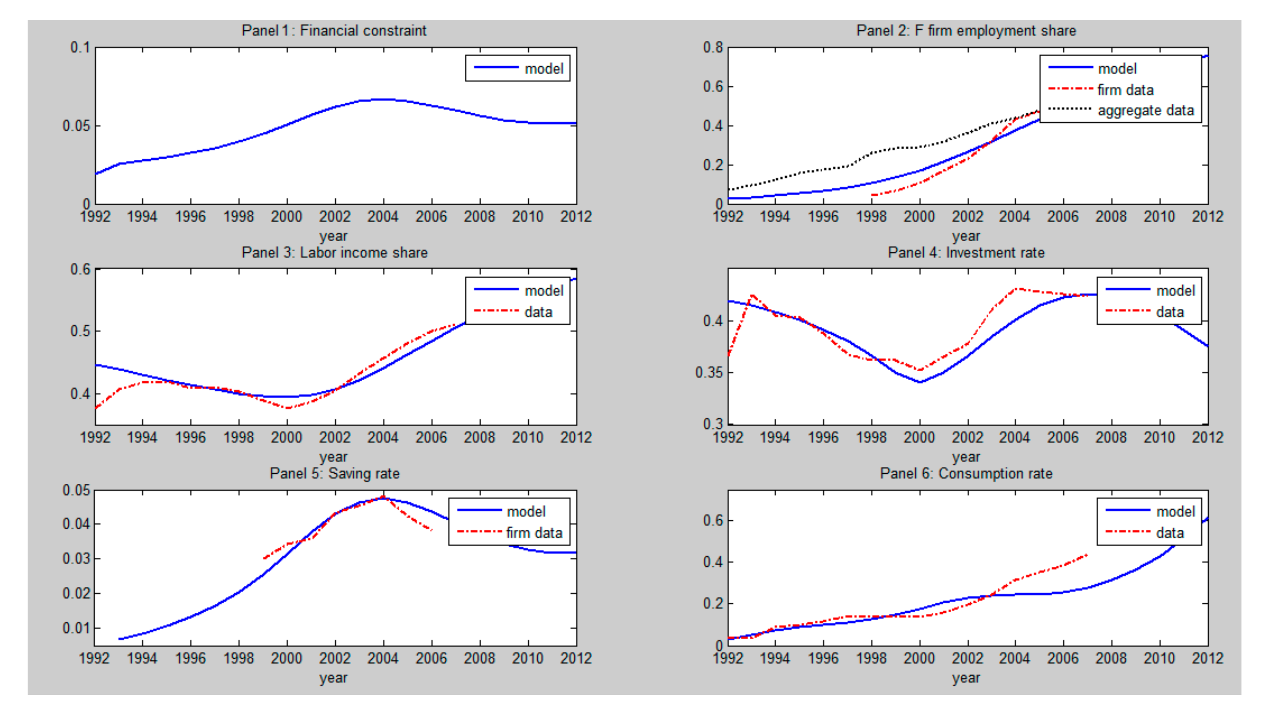Figure 10 describes the transformation dynamic path of employment, wage, investment, labor income share, savings rate and foreign reserve. Due to the financial constraint, Enterprise F can only obtain endogenous financing by occupying the laborers’ remuneration, which leads to the decrease of the labor income share. Thus, in the transformation, the labor income share is decreasing constantly (shown in Panel 3 of the Figure 10). After the transformation, all laborers will be employed by Enterprise F. In the transformation stage, the employment of Enterprise F will increase (shown in Panel 2 of Figure 10). In the meantime, the total savings rate $\raisebox{1ex}{$S_t$}\!\left/ \!\raisebox{-1ex}{$Y_t$}\right.$($S_t={\xi }^w{w}_t{N}_t+{\xi }_t^E\phi m_t$) increases constantly (shown in Panel 5 in Figure 10). The opposite investment rate $\raisebox{1ex}{$I_t$}\!\left/ \!\raisebox{-1ex}{$Y_t$}\right.$($I_{Ft}=k_{Ft+1}+k_{St+1}$) will decrease (shown in Panel 4 in Figure 10).

During the period of economic transformation, employment personnel are constantly allocated to F enterprise, and state-owned banks’ investment in S enterprise is constantly declining, which leads to a decline in the number of domestic loans. However, due to financial constraints, the number of loans to F enterprise is small. With the end of economic transformation, all the labor force is employed by F enterprise. With the continuous improvement of the financial market and the removal of financial constraints, F enterprise is no longer inclined to conduct endogenous financing by “crowding out” the remuneration of workers, and the savings rate will gradually decrease. In the stage of economic transformation, the continuous improvement of financial market will change the current situation in which non-state-owned enterprises mainly use endogenous financing. This is reflected in the increasing borrowing share of non-state-owned enterprises, because non-state-owned enterprises can make more use of exogenous financing. In this process, the proportion of the non-state-owned sector is increasing, and will absorb more and more resources; as a result, its returns are rising.

When the economic transformation is over and all labor is absorbed by the non-state-owned enterprise sector, the increase in its investment will lead to a decline in the investment rate (as shown in Panel 4 in Figure 10). The exogenous financing proportion of non-state enterprises increases during the economic transformation will reduce the proportion of non-state enterprise endogenous financing, and lower funding costs will lead the saving rate of the non-state enterprises to drop year by year. The non-state-owned enterprises do not tend toward “crowding out” of laborers’ remuneration for endogenous financing. This will increase the share of workers’ remuneration in non-state-owned enterprises (Panel 3 in Figure 10). Finally, the obvious result is that as financial markets mature, wages of non-state-owned enterprises will rise and their reduced dependence on endogenous financing will lead to a decline in the savings rate (see Panel 5 in Figure 10).

Next, we turn to the prediction and numerical analysis of the model to explain the characteristics of China’s economy from 1990 to 2014. The model predicts well the high rise in China’s savings rate, the inverted U-shaped change of the investment rate, the U-shaped change of the labor income share, and the continuous increase in employment in the non-state-owned enterprise sector. Parameter settings are shown in

Table 6. Calibration values of model reference parameters.

Variables	v	β	$\mathit{\theta }$	$\mathit{\delta }$	r	T
Parameters	0.03	0.997	0.2	0.1	0.175	50

. The parameters are set as follows: one phase is one year, so that an individual, at the age of 28, will begin to work and then retire at the age of 78 (T = 50). In general, Chinese people work for 30 years and retire at the age of 58. The thesis presumes that r = 0.175, which refers to the one-year deposit rate between 1998–2005 (after deducting the CPI level). According to Bai et al. [69], the capital share is set as 0.5 and the capital depreciation rate is $\delta =0.1$ (World Bank Development Index report). Workers’ growth rate is v, and v = 0.03. Finally, the intertemporal elasticity of substitution is set as $\theta =0.2$. According to Song at el. [5], the discount factor $\beta =0.997$.

Dynamic simulated economy based on the above parameter settings is shown in Figure 10. Panel 1–Panel 6 is the data fitting of the key macroeconomic variables of the model. First, we simulate the financial constraints (see Panel 1 in Figure 10); it can thus be seen that, with the massive restructuring of China’s financial system since the mid-1990s [7], gradually tightening measures were taken(though the purpose of the reform was to strengthen credit efficiency first), the tendency of “centralization” appears in the financial sector [8] which has accompanied the trend of decentralization in the real economy. Due to the lack of substantial progress in the financing environment of China’s financial market, financial institutions give priority to state-owned enterprises as the target of capital delivery, while the financing environment or financial constraints of non-state-owned enterprises have not been improved accordingly. Tighter financial constraints have led to a decline in China’s labor income share.

However, with the improvement of China’s financial market, the degree of financing constraint will be reduced. Second, the labor share in the model’s simulation is consistent with its decline since the 1990s and is U-shaped. In particular, the labor income share has fallen sharply since 2002, coinciding with a disproportionate rise in the saving rate (see Panel 3 in Figure 10). Thirdly, compared with the actual employment, the simulated economy shows accelerated employment transfer and allocation (as shown in Panel 2 in Figure 10). Finally, the total savings rate shows an inverted U-shape because our simulation here matches the average savings rate. The falling savings rate since the 1990s has been accompanied by China’s low consumption rate (see Panel 6 in Figure 10). Financial constraints on non-state-owned enterprises led to an increase in the corporate savings rate, which ultimately contributed to China’s high savings rate. The year-on-year rise since 2000 has coincided with a steady decline in the labor share (see Panel 5 in Figure 10).

From the analysis above, it can be seen that the important feature of the distribution mechanism of the model we constructed is that the existence of financial constraints makes it difficult for capital to flow to enterprises with high production efficiency, and they tend to conduct endogenous financing by “crowding out” workers’ remuneration. With the development of China’s economic transformation, the level of financial development continues to improve, financing constraints continue to ease, entrepreneurs can obtain exogenous financing at a lower cost, and are not inclined to financing through “crowding out” laborers remuneration, causing labor income share decline to ease or even increase.

Model calibration and quantitative prediction show that with the acceleration and completion of China’s economic transformation, China’s savings rate will reach its peak and then decline, while the labor income share will bottom out and rise.

8. Conclusions

The general decline in labor income share is one of the major problems confronted by the global economy today. This paper used firm-level micro-data to explore the reasons for the decline in labor income share from the novel perspective of financial constraints and corporate savings.

In theory, we review the typical facts of the Chinese economy, sort out the possible economic link between the rise in the savings rate and the fall in the labor share, and put forward the viewpoints to be tested. In other words, the existence of financial constraints in China’s imperfect financial market makes non-state-owned enterprises with higher efficiency more inclined to conduct endogenous financing by “crowding out” workers’ remuneration. This is the deep cause for the continuous decline of labor income share since the mid-1990s. Subsequently, based on the diamond model and overlapping generation model, a theoretical model is constructed to introduce financial constraints into the cost of obtaining credit. Proposition 1 and Proposition 2 are then proposed to be tested. Specifically, Proposition 1 is that corporate savings will increase with the increase of financial constraints, and Proposition 2 is that the share of labor income declines as financial constraints increase.

Empirically, based on data from the Chinese Industrial Enterprises from 1999 to 2007, the empirical research finds that, consistent with the theoretical Proposition 1 and Proposition 2, the existence of financial constraints in China’s financial market makes more efficient non-state-owned enterprises more inclined to conduct endogenous financing by “crowding out” workers’ remuneration. This is directly responsible for the steady decline in the labor share since the mid-1990s.

Finally, we carry on the numerical simulation and make a forecast whose results show that in the process of China’s financial market continuing to improve, the financing method of non-state-owned enterprises will gradually be transformed from endogenous financing to exogenous financing, so that enterprises’ “crowding out” labor remuneration will gradually disappear. This will further reduce China’s savings rate, and the labor income share will bottom out eventually.

These research results theoretically explain the imbalance phenomenon that rising savings rate is accompanied by declining labor income share from the perspective of financial constraints in China. The model calibration and fitting prediction show that with the improvement of financing constraints, the labor income share will stop falling and will rise. In the past four decades, the labor income share in the global macro primary distribution of national income has declined significantly [2,3]. This research provides a new possible explanation for the decline of the global labor income share. Considering the large impact of declining labor income share on income inequality [40] and sustainable development caused by income inequality [41,42,43], the empirical results of this paper provide empirical evidence and policy paths for other developing countries with imperfection financial markets [65,66] to carry out financial system reform, increase labor income share and promote sustainable economic development.

This paper is a preliminary study on how financial constraints reduce labor income share, and the impact of financial market imperfections on the economy is comprehensive. Credit constraints may also distort industrial structure and induce technological progress bias, and ultimately affect labor income share, which will be our future research direction. In the context of financing constraints in most developing countries [65], this series of studies will help these countries speed up financial reform and promote sustainable economic development.

References

1. Kaldor, N. A model of economic growth. Econ. J. 1957, 67, 591–624. [Google Scholar] [CrossRef]
2. Blanchard, O.J.; Nordhaus, W.D.; Phelps, E.S. The medium run. Brook. Pap. Econ. Act. 1997, 1997, 89–158. [Google Scholar] [CrossRef] [Green Version]
3. Guscina, A. Effects of globalization on labor’s share in national income. IMF Work. Pap. 2006, 2006, 33. [Google Scholar] [CrossRef]
4. Bai, C.E.; Qian, Z.J. Factor distribution of national income: The Story behind statistics. Econ. J. 2009, 3, 27–41. [Google Scholar]
5. Song, Z.; Storesletten, K.; Zilibotti, F. Growing like china. Am. Econ. Rev. 2011, 101, 196–233. [Google Scholar] [CrossRef] [Green Version]
6. Luo, C.; Zhang, J. Declining labor share: Is China’s case different? China World Econ. 2010, 18, 1–18. [Google Scholar] [CrossRef]
7. Boyreau-Debray, G.; Wei, S.J. Pitfalls of a state-dominated financial system: The case of China. Natl. Bur. Econ. Res. 2005. [Google Scholar] [CrossRef]
8. Park, A.; Shen, M. Refinancing and decentralization: Evidence from China. J. Econ. Behav. Organ. 2008, 66, 703–730. [Google Scholar] [CrossRef]
9. Aziz, J.; Cui, L. Explaining China’s Low Consumption: The Neglected Role of Household Income; International Monetary Fund: Washington, DC, USA, 2007. [Google Scholar]
10. Solow, R.M. A skeptical note on the constancy of relative shares. Am. Econ. Rev. 1958, 48, 618–631. [Google Scholar]
11. Bai, C.E.; Qian, Z.J. Determinants of labor income share: Evidence from China’s provincial panel data. World Econ. 2010, 12, 3–27. [Google Scholar]
12. Li, D.K.; Liu, L.L.; Wang, H.L. U-shaped law of labor share evolution in GDP. Econ. Res. J. 2009, 44, 70–82. [Google Scholar]
13. Luo, C.Y.; Zhang, J. Labor income share in economic development: An Empirical Study based on China’s Industrial Data. Soc. Sci. China 2009, 4, 65–79. [Google Scholar]
14. Harrison, A.E. Has Globalization Eroded Labor’s Share? Some Cross-Country Evidence; University Library of Munich: Munich, Germany, 2005. [Google Scholar]
15. Jayadev, A. Capital account openness and the labour share of income. Camb. J. Econ. 2007, 31, 423–443. [Google Scholar] [CrossRef]
16. Decreuse, B.; Maarek, P. FDI and the labor share in developing countries: A theory and some evidence. Ann. D’économie Stat. 2015, 289–319. [Google Scholar] [CrossRef]
17. Elsby, M.W.L.; Hobijn, B.; Şahin, A. The decline of the US labor share. Brookings Pap. Econ. Act. 2013, 2013, 1–63. [Google Scholar] [CrossRef] [Green Version]
18. Zhao, Q.Y.; Zhang, J.W. A new explanation of the changing trend of China’s labor income share and its Driving mechanism: Based on the perspective of international trade and minimum wage. Financ. Res. 2013, 44–56. [Google Scholar]
19. Bentolila, S.; Saint-Paul, G. Explaining movements in the labor share. Contrib. Macroecon. 2003, 3, 11–25. [Google Scholar] [CrossRef] [Green Version]
20. Ferguson, W.D. Explaining the rising wage-productivity gap of the 1980s: Effects of declining employment and unionization. Rev. Radic. Political Econ. 1996, 28, 77–115. [Google Scholar] [CrossRef]
21. Zavodny, M. Unions and the wage-productivity gap. Economic Review-Federal. Reserve Bank Atlanta 1999, 84, 44. [Google Scholar]
22. Fichtenbaum, R. Do unions affect labor’s share of income: Evidence using panel data. Am. J. Econ. Sociol. 2011, 70, 784–810. [Google Scholar] [CrossRef]
23. McCallum, J. Wage Gaps, Factor Shares and Real Wages//Trade Unions, Wage Formation and Macroeconomic Stability; Macmillan, P., Ed.; Palgrave Macmillan: London, UK, 1986; pp. 294–317. [Google Scholar]
24. Acemoglu, D. Labor- and Capital-Augmenting Technical Change. J. Eur. Econ. Assoc. 2003, 1, 1–37. [Google Scholar] [CrossRef] [Green Version]
25. Zuleta, H. Factor saving innovations and factor income shares. Rev. Econ. Dyn. 2008, 11, 836–851. [Google Scholar] [CrossRef] [Green Version]
26. Huang, X.H.; Xu, S. Analysis of the causes of the decline of the proportion of Labor income in China—Based on the perspective of labor-saving technological progress. Econ. Res. J. 2009, 7, 34–44. [Google Scholar]
27. Zhang, L.; LI, J.Y.; XU, X.X. International trade, biased technological progress and factor income distribution. Econ. Q. 2012, 11, 409–428. [Google Scholar]
28. Gollin, D. Getting income shares right. J. Political Econ. 2002, 110, 458–474. [Google Scholar] [CrossRef] [Green Version]
29. Long, Z.H.; Zhou, H.M. Empirical study on precautionary savings of Urban residents in China. Econ. J. 2000, 11, 33–38. [Google Scholar]
30. Meng, X. Unemployment, consumption smoothing, and precautionary saving in urban China. J. Comp. Econ. 2003, 31, 465–485. [Google Scholar] [CrossRef]
31. Chamon, M.; Prasad, E. Why are saving rates of urban households in China rising? Natl. Bur. Econ. Res. 2008. Available online: https://doi.org/10.3386/w14546 (accessed on 23 December 2021). [CrossRef]
32. Wan, G.H.; Zhang, Y.; Niu, J.G. Liquidity constraints, uncertainty and Household consumption in China. Econ. Res. J. 2001, 11, 35–44. [Google Scholar]
33. Ai, C.; Wang, W. The over-sensitivity of Chinese household consumption under habitual preference: An analysis based on the provincial Dynamic Panel Data from 1995 to 2005. J. Quant. Tech. Econ. 2008, 25, 98–114. [Google Scholar]
34. Yu, Y.D.; Li, J. The Theory and Verification of the Consumption Function of Chinese Residents. Chin. Soc. Sci. 2000, 1, 123–133. [Google Scholar]
35. Wang, W.; Guo, X.Q. Income inequality and China’s high savings rate: A Theoretical and Empirical Study from the Perspective of targeted consumption. Manag. World 2011, 7–25. [Google Scholar] [CrossRef]
36. Kraay, A. Household saving in China. World Bank Econ. Rev. 2000, 14, 545–570. [Google Scholar] [CrossRef] [Green Version]
37. Modigliani, F.; Cao, S.L. The Chinese saving puzzle and the life-cycle hypothesis. J. Econ. Lit. 2004, 42, 145–170. [Google Scholar] [CrossRef] [Green Version]
38. Wang, W. A Review of Researches on the Influence of Income Distribution on Savings Rate. J. Shanghai Univ. Financ. Econ. Philos. Soc. Sci. Ed. 2010, 12, 89–96. [Google Scholar]
39. Li, Y.; Yin, J.F. Research on China’s high savings rate—Analysis of China’s capital flow scale from 1992 to 2003. Econ. Res. J. 2007, 6, 14–26. [Google Scholar]
40. Doan, H.; Wan, G. Globalization and the Labor Share in National Income; Asian Development Bank Institute: Tokyo, Japan, 2017; Available online: https://www.adb.org/sites/default/files/publication/223671/adbi-wp639.pdf (accessed on 23 December 2021).
41. Walker, G. Inequality, Sustainability and Capability: Locating Justice in Social Practice//Sustainable Practices; Routledge: London, UK, 2013; pp. 197–212. [Google Scholar]
42. Martins, N.O. Inequality, sustainability and Piketty’s capital. Ecol. Econ. 2015, 118, 287–291. [Google Scholar] [CrossRef] [Green Version]
43. Masud MA, K.; Nurunnabi, M.; Bae, S.M. The effects of corporate governance on environmental sustainability reporting: Empirical evidence from South Asian countries. Asian J. Sustain. Soc. Responsib. 2018, 3, 3. [Google Scholar] [CrossRef]
44. Morel, L. A Sectoral Analysis of Labour’s Share of Income in Canada; Working Paper of Research Department; Bank of Canada: Ottawa, ON, Canada, 2005. [Google Scholar]
45. Boldrin, M.; Ruiz, C.G. What If Factor Shares Are Not Constant? Implications for Growth and Business Cycle Theories; Working Paper of University of Minnesota; Minnesota Press: Minneapolis, MN, USA, 2006. [Google Scholar]
46. Liu, Y.L.; Mao, R.; Yao, Y. Structural Transformation, financial crisis and the change of China’s labor income share. China Econ. Q. 2018, 17, 609–632. [Google Scholar]
47. Giammarioli, N.; Messina, J.; Steinberger, T. European Labor Share Dynamics: An Institutional Perspective; Economics Working Paper; European University Institute: Fiesole, Italy, 2002. [Google Scholar]
48. Blanchard, O.; Giavazzi, F. Macroeconomic Effects of Regulation and Deregulation in Goods and Labor Markets. Q. J. Econ. 2003, 118, 879–907. [Google Scholar] [CrossRef] [Green Version]
49. Bassanini, A.; Duval, R. Employment Patterns in OECD Countries: Reassessing the Role of Policies and Institutions. OECD Soc. Employ. Migr. Work.Pap. 2006, 127. [Google Scholar]
50. Schneider, D. The Labor Share: A Review of Theory and Evidence; SFB 649 Discussion Paper; Humboldt University: Berlin, Germany, 2011. [Google Scholar]
51. Zhang, S.F.; Lu, X.Q. Changes in labor income share in China: Technology bias or market distortion. Economist 2016, 15–24. [Google Scholar]
52. Diwan, I. Labor Income Shares and Globalization; World Bank Working Paper: Washington, DC, USA, 2000. [Google Scholar]
53. Diwan, I. Debt as Sweat: Labor, Financial Crises, and the Globalization of Capital; World Bank Working Paper: Washington, DC, USA, 2001. [Google Scholar]
54. Zhao, Q.Y.; WEI, X.H.; Zhang, J.W. International Trade, wage rigidity and labor income share. Nankai Econ. Res. 2012, 37–52. [Google Scholar]
55. Yu, M.J.; Liang, Z.H. Trade liberalization and China’s labor income share: An empirical analysis based on the data of manufacturing trade firms. Manag. World 2014, 22–31. [Google Scholar]
56. Jiang, W.; Huang, J.L. International production segmentation, factor endowment and labor income share: A theoretical and empirical study. World Econ. 2014, 37, 28–50. [Google Scholar]
57. Chen, H.; Wang, Y. Research on the Evolution characteristics and industry differences of China’s manufacturing technology progress. Sci. Res. 2015, 33, 859–867. [Google Scholar]
58. Acemoglu, D. Why Do New Technologies Complement Skills? Directed Technical Change and Wage Inequality. Q. J. Econ. 1998, 113, 1055–1089. [Google Scholar] [CrossRef] [Green Version]
59. Acemoglu, D. Technical Change, Inequality and the Labor Market. J. Econ. Lit. 2002, 40, 7–72. [Google Scholar] [CrossRef]
60. Acemoglu, D. Equilibrium Bias of Technology. Econometrica 2007, 75, 1371–1409. [Google Scholar] [CrossRef] [Green Version]
61. Aghion, P.; Bolton, P.A. Theory of Trickle-Down Growth and Development. Rev. Econ. Stud. 1997, 64, 151–172. [Google Scholar] [CrossRef] [Green Version]
62. Garnaut, R. Twenty Years of Economic Reform and Structural Change in the Chinese Economy. In Growth without Miracles; Garnaut, R., Huang, Y., Eds.; Oxford University Press: New York, NY, USA, 2001; pp. 1–18. [Google Scholar]
63. Luo, C.Y.; Chen, L. Will financing constraints lead to a lower share of labor income? J. Financ. Res. 2012, 29–42. [Google Scholar]
64. Abiad, A.; Mody, A. Financial reform: What shakes it? What shapes it? Am. Econ. Rev. 2005, 95, 66–88. [Google Scholar] [CrossRef]
65. Abiad, A.; Bluedorn, J.; Guajardo, J. The rising resilience of emerging market and developing economies. World Dev. 2015, 72, 1–26. [Google Scholar] [CrossRef]
66. Bartram, S.M.; Hou, K.; Kim, S. Real effects of climate policy: Financial constraints and spillovers. J. Financ. Econ. 2021. [Google Scholar] [CrossRef]
67. Kuijs, L. Investment and Saving in China; Working Paper Series 3633; The World Bank Office Beijing: Beijing, China, 2005; Available online: https://documents1.worldbank.org/curated/en/644241468213285959/pdf/wps3633.pdf (accessed on 23 December 2021).
68. Hofman, B.; Kuijs, L. Rebalancing China’s Growth. In Debating China’s Exchange Rate Policy; Goldstein, M., Lardy, N.R., Eds.; Peterson Institute for International Economics: Washington, DC, USA, 2008; pp. 109–121. [Google Scholar]
69. Bai, C.E.; Qian, Z.J.; Wu, K.P. Research on the Determinants of China’s Industrial Sector Distribution of Factors. Econ. Res. J. 2008, 8, 16–28. [Google Scholar]
70. Wan, J.T.; Wei, X.H. The impact of minimum wage regulation on enterprise labor income share: Theoretical analysis and micro-evidence. Study Financ. Econ. 2020, 46, 64–78. [Google Scholar]
71. Zhou, M.; Li, Y.; Yao, X.; Lu, Y. Human Capital expansion and Manufacturing export upgrading in Chinese cities: Evidence from university enrollment expansion. Manag. World 2019, 35, 64–77. [Google Scholar]
72. Modigliani, F.; Miller, M.H. The cost of capital, corporation finance and the theory of investment. Am. Econ. Rev. 1958, 48, 261–297. [Google Scholar]
73. Allen, F.; Qian, J.; Qian, M. Law, finance, and economic growth in China. J. Financ. Econ. 2005, 77, 57–116. [Google Scholar] [CrossRef] [Green Version]
74. Lu, F.; Yao, Y. The rule of law, financial Development and economic Growth under financial repression. Soc. Sci. China 2004, 42–55. [Google Scholar]
75. Dollar, D.; Wei, S.J. Das (wasted) Kapital: Firm ownership and investment efficiency in China; National Bureau of Economic Research: Cambridge, MA, USA, 2007. [Google Scholar] [CrossRef]
76. Riedel, J.; Jin, J.; Gao, J. How China Grows: Investment, Finance, and Reform. China Q. 2008, 196, 924–956. [Google Scholar]
77. Aziz, J.; Li, X. China’s Changing Trade Elasticities; International Monetary Fund: Washington, DC, USA, 2007. [Google Scholar]
78. Shao, M.; Bao, Q.; Ye, N.H. The impact of credit financing constraints on employee income: Empirical evidence from the micro-level of Chinese enterprises. Econ. Q. 2013, 12, 895–912. [Google Scholar]
79. Wei, X.H.; Dong, Z.Q.; Huang, J.L. Does trade union improve labor income share?—Theoretical analysis and empirical evidence from Chinese private enterprises. Econ. Res. 2013, 48, 16–28. [Google Scholar]
80. Judd, C.M.; Kenny, D.A. Process analysis: Estimating mediation in treatment evaluations. Eval. Rev. 1981, 5, 602–619. [Google Scholar] [CrossRef]
81. Baron, R.M.; Kenny, D.A. The moderator–mediator variable distinction in social psychological research: Conceptual, strategic, and statistical considerations. J. Personal. Soc. Psychol. 1986, 51, 1173. [Google Scholar] [CrossRef]
82. Wang, W.; Guo, X.Q.; Ai, C.R. Financial constraints, labor income share decline and China’s low consumption. Econ. Res. 2013, 48, 100–113. [Google Scholar]
83. Nie, H.H.; Jiang, T.; Yang, R.D. The application status and potential problems of China’s industrial enterprise database. World Econ. 2012, 35, 142–158. [Google Scholar]
84. Lu, X.D.; Lian, Y.J. Estimation of total factor productivity of industrial enterprises in China: 1999–2007. China Econ. Q. 2012, 11, 541–558. [Google Scholar]
85. Huang, L.; Liu, S.; Han, Y. The nature of state-owned enterprises and collection of pollutant discharge fees: A study based on Chinese industrial enterprises. J. Clean. Prod. 2020, 271, 122420. [Google Scholar] [CrossRef]
86. Ai, H.; Hu, S.; Li, K. Environmental regulation, total factor productivity, and enterprise duration: Evidence from China. Bus. Strategy Environ. 2020, 29, 2284–2296. [Google Scholar] [CrossRef]
87. Wen, Y.B.; Lu, X.Q. An analysis of the determinants of labor income share change in China: A dual perspective of market competition and institutional quality. Econ. Res. J. 2018, 53, 83–98. [Google Scholar]
Figure 1. China: Labor income share and national savings rate (1993–2007). Sources: China’s Statistical Yearbook: 1993–2007, China Compendium of Statistics and World Bank Database. Notes: National savings rate 1 shall be calculated in accordance with expenditure GDP and final consumption rate; national savings rate 2 shall be calculated in accordance with China’s fund flow statements; national savings rate 3 is from the World Bank Database.
Sustainability 14 00346 g001
Figure 2. Saving rates by sector in China from 1992 to 2007. Sources: Calculated according to the statement of capital flow.
Sustainability 14 00346 g002
Figure 3. Proportion of various components in the initial distribution of income by the enterprise sector. Sources: Calculated according to the statement of capital flow.
Sustainability 14 00346 g003
Figure 4. Decomposing China’s labor income share by sector from 1992 to 2007. Sources: Calculated according to the statement of capital flow.
Sustainability 14 00346 g004
Figure 5. Corporate labor income share for the total enterprises, SOE and Non-SOE. Note: SOE includes state-holding enterprises and collectivity-holding enterprises. Non-SOE includes enterprises that are held by private holding, foreign holding, Hong Kong–Macao–Taiwan holding and other holding. Sources: China Industrial Economy Statistical Yearbook (1999–2003; 2003–2007).
Sustainability 14 00346 g005
Figure 6. Savings rate of all enterprises, state-owned enterprises and non-state-owned enterprises. Note: State-owned enterprises include state-owned holding enterprises and collective holding enterprises. Non-state-owned enterprises include private holding, foreign holding, Hong Kong, Macao and Taiwan holding and other holding. Source: China Industrial Enterprise Database (1999–2003; 2003–2007).
Sustainability 14 00346 g006
Figure 7. Percent of investment financed by banks. Sources: China’s Statistical Yearbook: 1997–2007; China’s economy and trade Statistical Yearbook: 1997–2007.
Sustainability 14 00346 g007
Figure 8. Labor income share change of listed companies in China. Data sources: Labor share 1 is derived from the CSMAR database; Labor share 2 is derived from financial data of CCER general listed companies.
Sustainability 14 00346 g008
Figure 9. Mediating effect.
Sustainability 14 00346 g009
Figure 10. Transition in the calibrate economy. Notes: Panel 1 refers to financial constraints; Panel 2 refers to the employment of Enterprise F; Panel 3 refers to the labor income share; Panel 4 refers to the investment rate; Panel 5 refers to the savings rate; Panel 6 refers to the savings rate. All data are firstly logarithmic, then the HP filter is removed.
Sustainability 14 00346 g010