
Spatio-Temporal Variations of Discharge and Sediment in Rivers Flowing into the Anzali Lagoon


Abstract
:1. Introduction
2. Materials and Methods
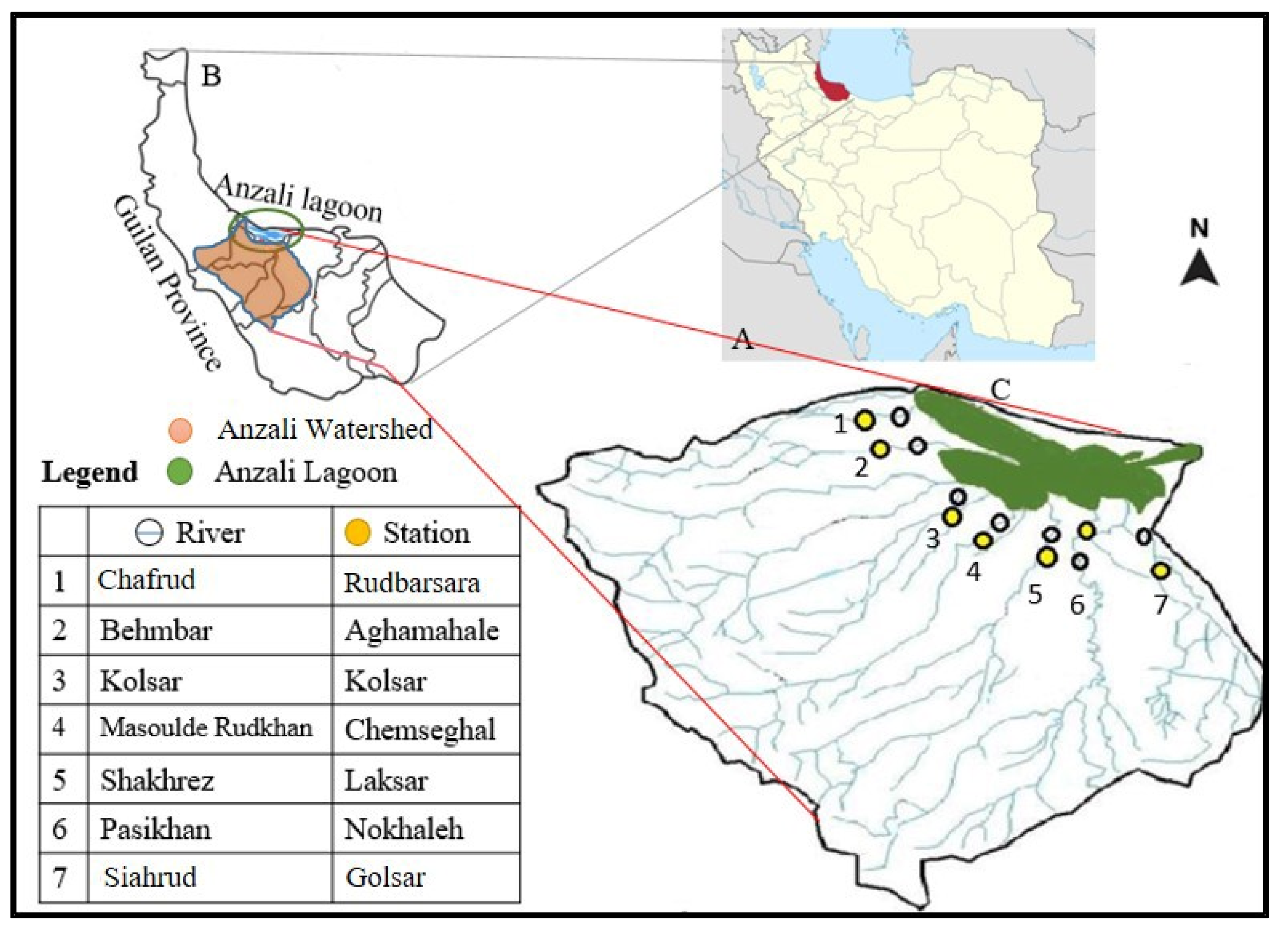
2.1. Study Area
2.2. Data Collection
2.3. Data Analysis
2.3.1. Mann–Kendall Test
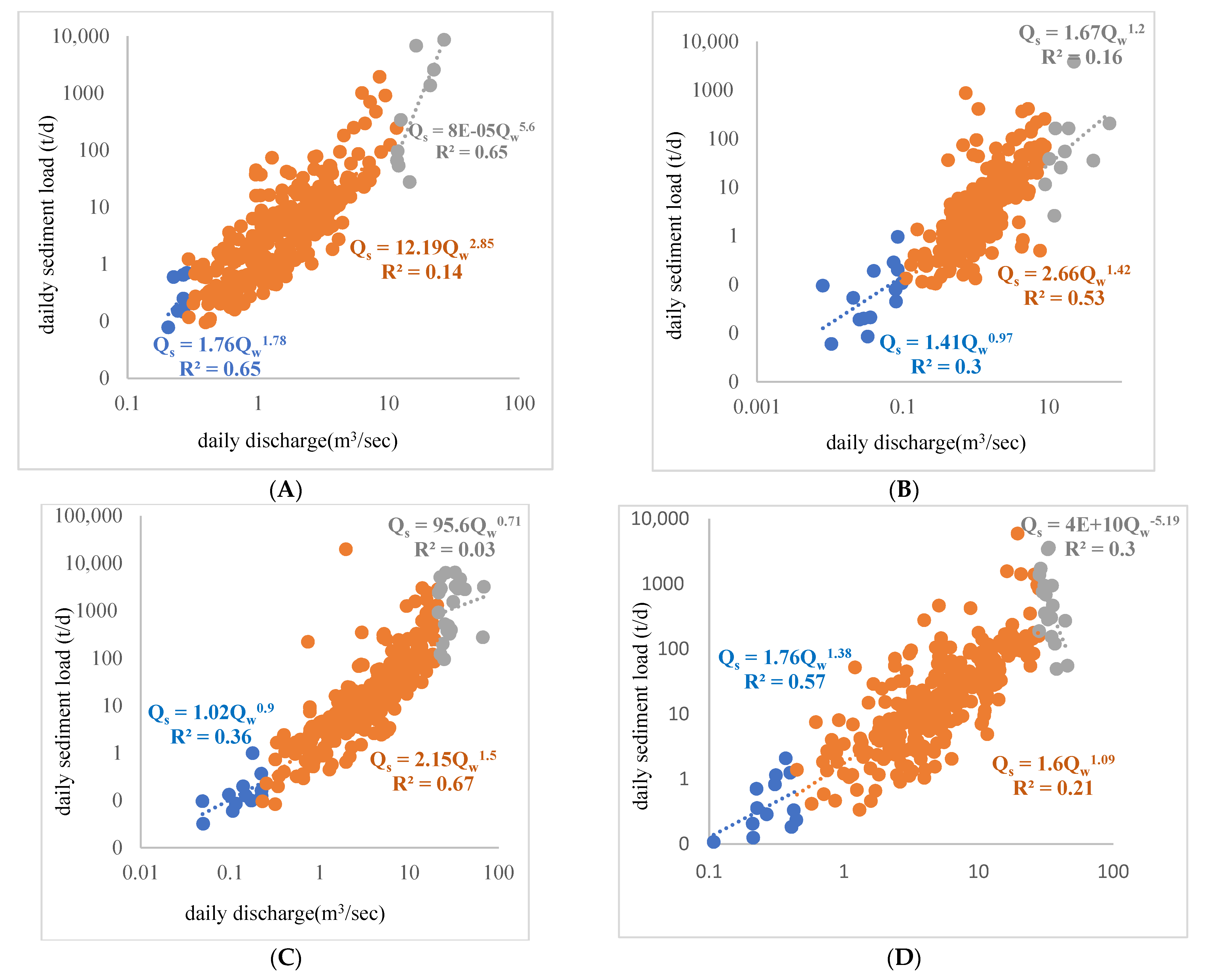
2.3.2. Double-Mass Curve
3. Results
4. Conclusions
Author Contributions
Funding
Institutional Review Board Statement
Informed Consent Statement
Data Availability Statement
Conflicts of Interest
References
- Arnild, J.G. Water resources of the Texas Gulf Basin. Water Sci. Technol. 1999, 39, 121–133. [Google Scholar] [CrossRef]
- Zhai, H.J.; Hu, B.; Luo, X.Y.; Qiu, L.; Tang, W.J.; Jiang, M. Spatial and temporal changes in runoff and sediment loads of the Lancang River over the last 50 years. Agric. Water Manag. 2016, 174, 74–81. [Google Scholar] [CrossRef]
- Amin, S.A.; Mirzaii, H. Measure and estimate the temporal variation of suspended sediment using Sediment curve approach in the Merg River. Geogr. Environ. Sustain. 2017, 3, 13–22. (In Persian) [Google Scholar]
- Refahi, H.G. Water Erosion and Conservation; University of Tehran Publication: Tehran, Iran, 1996. [Google Scholar]
- Crowder, D.; Demissiie, W.; Markus, M. The accuracy of sediment load when log transformation produces nonlinear sediment load-discharge relationship. Hydrology 2007, 336, 250–268. [Google Scholar] [CrossRef]
- Piri, A.; Habibnezhad, M.; Ahmadi, M.; Soleimani, K.; Mosaedi, A. Optimizing the relationship between water discharge and sediment load in Amameh. J. Khazar Agric. Sci. Nat. Resour. 2005, 3, 30–40. [Google Scholar]
- Crawford, C.G. Estimation of suspended sediment rating curves and mean suspended sediment loud. Hydrology 1991, 129, 331–348. [Google Scholar] [CrossRef]
- Vafakhah, M. Comparison of co-kriging and adaptive neuro-fuzzy inference system models for suspended sediment load forecasting. Arab. J. Geosci. 2013, 6, 3003–3018. [Google Scholar] [CrossRef]
- Tuset, J.; Vericat, D.; Batalla, R.J. Rainfall, runoff and sediment transport in a Mediterranean mountainous catchment. Sci. Total Environ. 2016, 540, 114–132. [Google Scholar] [CrossRef] [PubMed]
- Williams, G.P. Sediment concentration versus water discharge. Hydrology 1989, 111, 89–106. [Google Scholar] [CrossRef]
- Mohamadi, A.; Mosaedi, A.; Heshmatpour, A. Determination of the best model to estimate suspended sediment load in Ghazaghli gauge station Gorganroud river. Agric. Sci. Nat. Resour. 2007, 14, 232–240. (In Persian) [Google Scholar]
- Fleming, G. Deterministic model in hydrology. Food Agric. Organ. United Nations 1979, 32, 32–80. [Google Scholar]
- Walling, D.E. Suspended sediment and solute response characteristics of the river Exe, Devon, England. In Research in Fluvial Geomorphology (Proceedings of the 5th Guelph Symposium on Geomorphology); Davidson-Arnott, R., Nickling, W., Eds.; Geoabstracts: Norwich, UK, 1978; pp. 169–197. [Google Scholar]
- Asselman, M.E.M. Fitting and interpretation of sediment rating curves. Hydrology 2002, 234, 228–248. [Google Scholar] [CrossRef]
- Robert, B.T. Estimating total suspended sediment yield with probability sampling. Water Resour. Res. 1985, 21, 1381–1388. [Google Scholar]
- Fang, N.F.; Shi, Z.H.; Lu., L.; Cheng, J. Rainfall, runoff and suspended sediment delivery relationships in a small agricultural watershed of the Three Gorges area, China. Geomorphology 2011, 135, 158–166. [Google Scholar] [CrossRef]
- Lana-Renault, N.; Regues, D.; Nadal-Romero, E.; Serrano-Muela, M.P.; Garcia-Ruiz, J.M. Streamflow response and sediment yield after farmland abandonment: Results from a small experimental catchment in the central Spanish Pyrenees. Pirin. Rev. De Ecol. De Mont. 2010, 165, 97–114. [Google Scholar] [CrossRef] [Green Version]
- Liu, C.; Wang, Z.Y.; Sui, J.Y. Analysis on variation of seagoing water and sediment load in main rivers of China. Hydraul. Eng. 2007, 38, 1444–1452. [Google Scholar]
- Roy, N.G.; Sinha, R. Effective discharge for suspended sediment transport of the Ganga River and its geomorphic implications. Geomorphology 2014, 4, 221–234. [Google Scholar] [CrossRef]
- Wu, B.; Wang, G.; Xia, J.; Fu, X.; Zhang, Y. Response of bankfull discharge to discharge and sediment load in the Lower Yellow River. Geomorphology 2008, 100, 366–376. [Google Scholar] [CrossRef]
- Yuan, Z.J.; Chu, Y.M.; Shen, Y.J. Simulation of surface runoff and sediment yield under different land-use in a Taihang Mountains watershed North China. Soil Tillage Res. 2015, 153, 7–19. [Google Scholar] [CrossRef]
- Tian, S.; Xu, M.; Jiang, E.; Wang, G.; Hu, H.; Liu, X. Temporal variations of runoff and sediment load in the upper Yellow River, China. Hydrology 2019, 568, 46–56. [Google Scholar] [CrossRef]
- Namsai, M.; Bidorn, B.; Chanyotha, S.; Mama, R. Sediment dynamics and temporal variation of runoff in the Yom River. Thailand. Int. J. Sediment Res. 2020, 35, 365–376. [Google Scholar] [CrossRef]
- Noori, H.; Siadatmousavi, S.M.; Mojaradi, B. Assessment of sediment yield using RS and GIS at two sub-basins of Dez Watershed, Iran. Int. Soil Water Conserv. Res. 2016, 4, 199–206. [Google Scholar] [CrossRef] [Green Version]
- Japan International Cooperation Agency (JICA). The study on integrated management for ecosystem conservation of the Anzali wetland in the Islamic republic of Iran. In Final Report: Executive Report; 2005. Available online: https://openjicareport.jica.go.jp/pdf/11784097.pdf (accessed on 19 October 2021).
- Grave, D.S.; Ghane, A. The establishment of the Oriental River Prawn, Macrobrachium nipponense (de Haan, 1849) in Anzali Lagoon, Iran. Aquat. Invasions 2007, 1, 204–208. [Google Scholar] [CrossRef]
- Marzvan, S.; Moravej, K.; Felegari, S. Risk Assessment of Alien Azolla filiculoides Lam in Anzali Lagoon Using Remote Sensing Imagery. Indian Soc. Remote. Sens. 2021, 49, 1801–1809. [Google Scholar] [CrossRef]
- Rafiei, B.; Ghomi, F.A.; Ardebili, L.; Sadeghifar, M.; Sharifi, S.H.K. Distribution of Metals (Cu, Zn, Pb, and Cd) in Sediments of the Anzali Lagoon, North Iran. Soil Sediment Contam. 2012, 21, 768–787. [Google Scholar] [CrossRef]
- Haji, K.; Mostafazade, R.; Esmaeeli, A.; Mirzaii, S. Temporal and spatial variations in the intensity of monthly discharge and sediment concentrations in a number of Hydrometric stations of West Azerbaijan province. Watershed Eng. Manag. 2019, 11, 619–632. (In Persian) [Google Scholar]
- Sobhani, M.; Tajbakhsh, S.M.; Memarian, H. Statistical Trend Analysis of Suspended Sediment Load in Association with Watershed Management Practices (Case Study: Bar Watershed, Neyshabur, Iran). Iran-Watershed Manag. Sci. Eng. 2017, 11, 69–84. (In Persian) [Google Scholar]
- Abbasi, A. 210Pb and 137Cs based techniques for the estimation of sediment chronologies and sediment rates in the Anzali Lagoon, Caspian Sea. Radio Anal. Nucl. Chem. 2019, 322, 319–330. [Google Scholar] [CrossRef]
- Vavdare, S.K.; Sedghi, H.; Sarraf, P. Determination of Sedimentation Rate in Anzali Lagoon of Northern Iran using 137Cs Tracer Technique. Appl. Ecol. Environ. Res. 2019, 17, 1337–1347. [Google Scholar] [CrossRef]
- Rob, J.H.; Koehler, A.B. Another look at measures of forecast accuracy. Int. J. Forecast. 2006, 22, 679–688. [Google Scholar]
- Willmott, C.J.; Matsuura, K. Advantages of the mean absolute error (MAE) over the root mean square error (RMSE) in assessing average model performance. Clim. Res. 2005, 30, 79–82. [Google Scholar] [CrossRef]
- Schaeffer, D.L. A model evaluation methodology applicable to environmental assessment models. Ecol. Model. 1980, 8, 275–295. [Google Scholar] [CrossRef] [Green Version]
- Loague, K.; Green, R.E. Statistical and graphical methods for evaluating solute transport models: Overview and application. Contam. Hydrol. 1991, 7, 51–73. [Google Scholar] [CrossRef]
- Kendall, M.G. Rank Correlation Measures; Charles Griffin: London, UK, 1975; 202p. [Google Scholar]
- Mann, H.B. Nonparametric tests against trend. Econometrica 1945, 13, 245–259. [Google Scholar] [CrossRef]
- Jiang, C.; Zhang, L.; Li, D.; Li, F. Water discharge and sediment load changes in China: Change patterns, causes, and implications. Water 2015, 7, 5849–5875. [Google Scholar] [CrossRef] [Green Version]
- Shi, H.; Hu, C.; Wang, Y.; Liu, C.; Li, H. Analyses of trends and causes for variations in runoff and sediment load of the Yellow River. Int. J. Sediment Res. 2017, 32, 171–179. [Google Scholar] [CrossRef]
- Yue, X.; Mu, X.; Zhao, G.; Shao, H.; Gao, P. Dynamic changes of sediment load in the middle reaches of the Yellow River Basin, China and implications for eco-restoration. Ecol. Eng. 2014, 73, 64–72. [Google Scholar] [CrossRef]
- Zhang, L.; Li, S.; Wu, Z.; Fan, X.; Li, H.; Meng, Q.; Wang, J. Variation in Runoff, Suspended Sediment Load, and Their Inter-Relationships in Response to Climate Change and Anthropogenic Activities over the Last 60 Years: A Case Study of the Upper Fenhe River Basin, China. Water 2020, 12, 1757. [Google Scholar] [CrossRef]
- Hirsch, R.M.; Smith, R.A.; Slack, J.R. Techniques of trend analysis for monthly water quality data. Water Resour. 1982, 18, 107–121. [Google Scholar] [CrossRef] [Green Version]
- Gan, T.Y. Finding Trends in Air Temperature and Precipitation for Canada and Northeastern United States. In Using Hydrometric Data to Detect and Monitor Climate Change. Proceedings of NHRI Workshop No. 8; Kite, G.W., Harvey, K.D., Eds.; National Hydrology Research Institute: Saskatoon, SK, Canada, 1992; pp. 57–78. [Google Scholar]
- Prashanth, K. Mann-Kendall Analysis for the Fort Ord Site. HydroGeoLogic, Inc, Annual Groundwater Monitoring Report; Army Corps of Engineers: Herndon, VA, USA, 2005; pp. 1–7. [Google Scholar]
- Gao, J.H.; Jia, J.; Kettner, A.J.; Xing, F.; Wang, F. Reservoir-induced changes to fluvial fluxes and their downstream impacts on sedimentary processes: The Changjiang (Yangtze) River, China. Quat. Int. 2015, 493, 187–197. [Google Scholar] [CrossRef]
- Huo, Z.; Feng, S.; Kang, S.; Li, W.; Chen, S. Effect of climate changes and water-related human activities on annual stream flows of the Shiyang River basin in arid north-west China. Hydrol. Processes 2008, 22, 3155–3167. [Google Scholar] [CrossRef]
- Li, D.; Lu, X.X.; Yang, X.; Chen, L.; Lin, L. Sediment load responses to climate variation and cascade reservoirs in the Yangtze River: A case study of the Jinsha river. Geomorphology 2018, 322, 41–52. [Google Scholar] [CrossRef]
- Zhao, Y.; Zou, X.; Liu, Q.; Yao, Y.; Li, Y.; Wu, X.; Wang, C.; Yu, W.; Wang, T. Assessing natural and anthropogenic influences on water discharge and sediment load in the Yangtze River, China. Sci. Total Environ. 2017, 607–608, 920–932. [Google Scholar] [CrossRef]
- Li, Z.; Xu, X.; Yu, B.; Xu, C.; Liu, M.; Wang, K. Quantifying the impacts of climate and human activities on water and sediment discharge in a karst region of Southwest China. Hydrology 2016, 542, 836–849. [Google Scholar] [CrossRef]
- Zabardast, L.; Jafari, H.R. Evaluating the trend of changes in Anzali Wetland using remote sensing and providing management solutions. Environ. Sci. 2011, 57, 57. (In Persian) [Google Scholar]
- Shakeri, R.; shayesteh, K.; ghorbani, M. Assessment and prediction of land use changes in the Anzali wetland Basin, Based on Land Change Modeler (LCM). Iran. J. Remote Sens. GIS 2019, 11, 93–114. (In Persian) [Google Scholar]
- Jamieson, P.D.; Porter, J.R.; Wilson, D.R. A test of the computer simulation model Arcwheat 1 on wheat crops grown in New Zealand. Field Crops Res. 1991, 27, 337–350. [Google Scholar] [CrossRef]
- Searcy, J.K.; Hardison, C.H.; Langbein, W.B. Double-Mass Curves. In Manual of Hydrology: Part 1. General Surface- Water Techniques; Geological Survey Water-Supply paper 1541-b; United States Government Printing Office: Washington, DC, USA, 1960; 41p. [Google Scholar]


| Rivers | Stations | Longitude | Latitude | Elevation (m) | Average Discharge (m3/s) | Average Sediment Load (t/day) |
|---|---|---|---|---|---|---|
| Behmbar | Aghamahale | 343,802 | 4,147,503 | −15 | 2.9 | 31.9 |
| Masoulde Rudkhan | Chemseghal | 355,172 | 4,137,526 | −22 | 6.5 | 265.01 |
| Kolsar | Kolsar | 351,742 | 4,140,028 | −23 | 8.12 | 118.2 |
| Shakhrez | Laksar | 360,196 | 4,135,259 | −20 | 14.8 | 332.8 |
| Pasikhan | Nokhaleh | 362,962 | 4,134,794 | −20 | 27.9 | 874.8 |
| Chafrud | Rudbarsara | 331,846 | 4,152,616 | −20 | 2.6 | 88.5 |
| Siahrud | Golsar | 374,668 | 4,128,805 | −20 | 6.44 | 263.57 |
| Station | Parameter | Mar | Apr. | May | Jun. | Jul. | Aug. | Sep. | Nov. | Oct. | Dec. | Jan. | Feb. |
|---|---|---|---|---|---|---|---|---|---|---|---|---|---|
| Rudbarsara | Discharge | 0.68 | 1.92 | −1.04 | 1.16 | −2.05 * | −0.18 | 0.61 | −0.31 | −0.4 | 0.6 | −1.53 | 0.93 |
| Sediment | 0.96 | 0.01 | 0.63 | 0.65 | −3.19 ** | −0.72 | −0.76 | 0.17 | −1.15 | −1.29 | −2.2 * | 0.56 | |
| Aghamahale | Discharge | 2.65 ** | 2.06 * | 3.08 ** | 0.87 | 0.45 | −0.06 | 0.65 | −0.42 | −1.17 | −1.68 | 0.58 | −0.75 |
| Sediment | 1.92 | 0.93 | 2.2 * | −1.19 | 0.08 | −0.48 | −0.16 | −0.44 | −0.75 | −1.14 | −0.03 | −0.9 | |
| Kolsar | Discharge | 1.10 | 1.40 | −2.53* | 0.98 | 0.62 | 1.09 | 1.05 | 1.34 | 1.15 | −0.05 | 0.56 | −1.61 |
| Sediment | 1.04 | 0.87 | −3.43 ** | −0.6 | 0.9 | 1.06 | 0.42 | −0.47 | 0.12 | −0.61 | 1.15 | −1.33 | |
| Chemseghal | Discharge | −0.19 | 0 | −0.19 | 1.86 | −0.3 | 1.15 | 0.8 | 1.23 | 0.77 | 0.04 | −1.07 | −2.21 * |
| Sediment | −0.37 | −0.25 | −0.77 | 1.65 | −0.62 | 0.76 | 0.52 | 0.01 | 0.21 | −0.25 | 0.83 | −2.42 * | |
| Golsar | Discharge | 0.27 | −0.15 | 0.3 | 1.36 | −0.53 | 0.99 | 0.43 | 1.18 | 0.49 | −0.18 | −1.26 | −2.2 * |
| Sediment | 0.28 | 0.25 | −0.09 | 1.65 | −0.62 | 1.03 | 0.16 | 0.01 | −0.06 | −0.53 | −0.7 | −2.39 * | |
| Laksar | Discharge | 0.22 | 2.42 * | 0.09 | −1.08 | −1.28 | −1.04 | −1.1 | −2.06 * | −3.29 ** | −0.91 | −2.11 * | −0.52 |
| Sediment | −0.03 | 2.28 * | −0.34 | −2.14 * | −1.6 | −1.65 | −0.27 | −2.31 * | −1.03 | −1.01 | −2.28 * | 0.04 | |
| Nokhaleh | Discharge | −1.47 | −0.06 | −2.25 * | −0.71 | −1.92 | 0.51 | 1.16 | 0.46 | 1.43 | −0.14 | −1.19 | −1.55 |
| Sediment | −2.18 * | −0.03 | −1.82 | −1.15 | −2.01 * | 1.63 | 1.19 | −0.08 | 1.16 | −0.48 | 0.06 | −1.58 |
| Station | Parameter | Annual | Spring | Summer | Fall | Winter |
|---|---|---|---|---|---|---|
| Rudbarsara | Discharge | −1.1 | −0.19 | −0.71 | −0.28 | −0.42 |
| Sediment | −3.2 ** | 0.5 | −2.5 * | −1.63 | −2.67 ** | |
| Aghamahale | Discharge | 0.14 | 2.48 | −0.82 | −0.33 | −0.93 |
| Sediment | −2.65 ** | 0.88 | −2.3 * | −0.79 | −0.96 | |
| Kolsar | Discharge | −0.64 | −1.5 | 0.65 | −0.37 | −0.34 |
| Sediment | −0.64 | −1.5 | 0.65 | −0.37 | −0.34 | |
| Chemseghal | Discharge | −0.71 | −0.58 | −0.34 | 1.47 | −0.85 |
| Sediment | −1.45 | −0.52 | −0.85 | −0.04 | −0.79 | |
| Golsar | Discharge | −0.65 | −0.37 | −0.73 | 0.92 | −1.14 |
| Sediment | −1.45 | 0.13 | −0.82 | −0.49 | −1.02 | |
| Laksar | Discharge | −0.92 | 0.4 | −1.57 | −1.62 | −1.5 |
| Sediment | −1.84 | −0.12 | −2.34 * | −1.5 | −1.23 | |
| Nokhaleh | Discharge | 0.08 | −2.03 * | −0.76 | 1.52 | −0.59 |
| Sediment | −1.38 | −2.06 * | −1.8 | 0.99 | −1.32 |
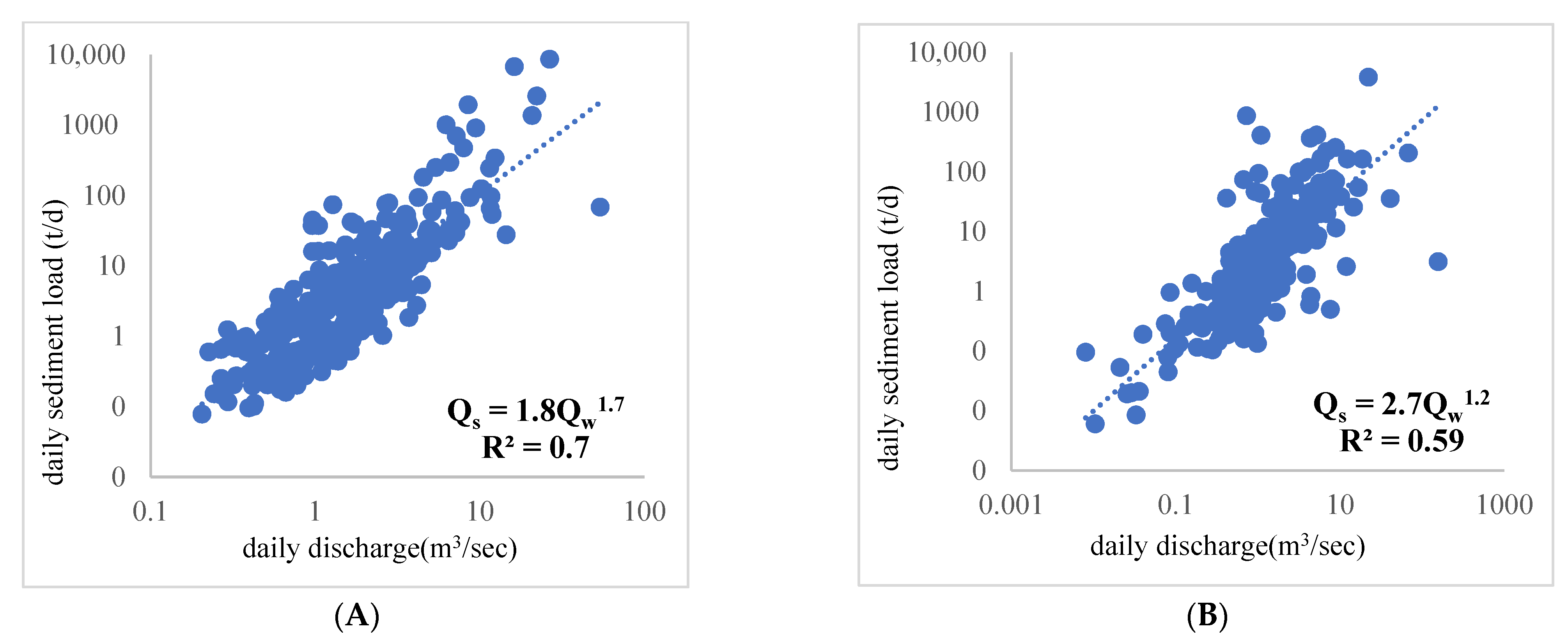
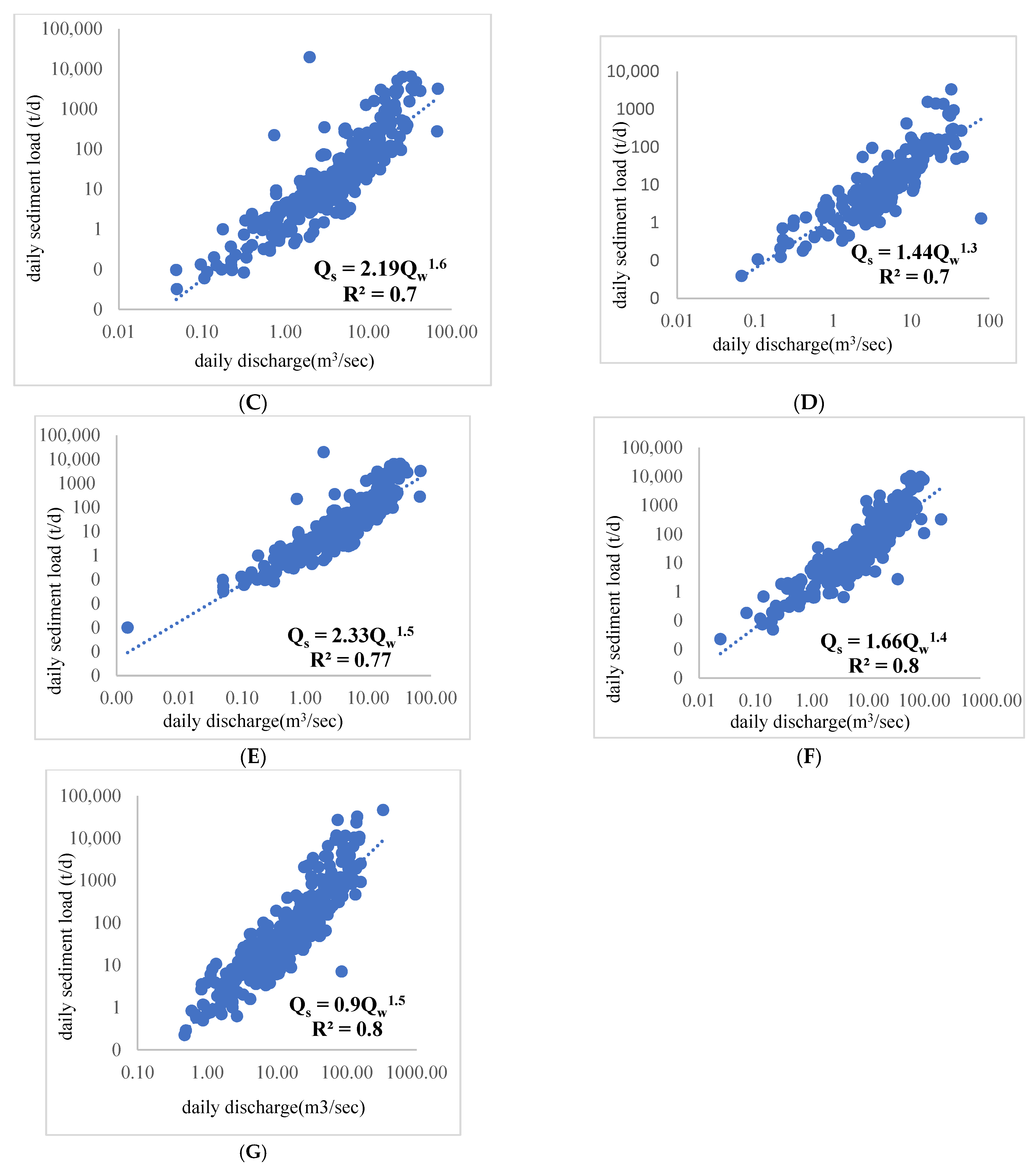
| Hydrometry Station | Polynomial Equation | R2 (%) | RMSE (t/d) | nRMSE (%) | MAE (%) | EF (%) |
|---|---|---|---|---|---|---|
| Rudbarsara | Qs = 1.80Qw1.77 | 0.7 | 6.37 | 0.95 | 0.21 | −0.31 |
| Aghamahale | Qs = 2.71Qw1.21 | 0.59 | 22.51 | 0.98 | 0.94 | −16.3 |
| Kolsar | Qs = 1.44Qw1.3 | 0.72 | 6.9 | 0.21 | 1.58 | 2.78 |
| Chemseghal | Qs = 2.19Qw1.6 | 0.76 | 1.55 | 0.14 | 0 | −0.11 |
| Golsar | Qs = 2.33Qw1.56 | 0.77 | 6.71 | 0.16 | 0.03 | −1.53 |
| Laksar | Qs = 1.66Qw1.46 | 0.8 | 6.93 | 0.12 | 0.01 | 1.43 |
| Nokhaleh | Qs = 0.90Qw1.58 | 0.79 | 9.11 | 0.17 | 0.02 | 1.49 |
| Station | Statistical Indices | Polynomial | Linear | Exponential | Logarithmic |
|---|---|---|---|---|---|
| Rudbarsara | Function | Qs = −2.01Qw2 + 142.63Qw − 235.79 | Qs = 72.25Qw − 100.8 | Qs = 1.9e0.2Qw | Qs = 218.82ln(Qw) − 10.9 |
| RMSE (t/d) | 180.62 | 96.69 | 12.35 | 67.68 | |
| nRMSE (%) | −1294.63 | 584.24 | 443.53 | 1271.9 | |
| EF (%) | 167.49 | 47.99 | 0.78 | 23.52 | |
| MAE (%) | 20.23 | −10.15 | 3.56 | 1.03 | |
| R2 | 0.3 | 2 | 0.3 | 0.1 | |
| Aghamahale | Function | Qs = −0.13Qw2 + 21.24Qw − 13.92 | Qs = 3.05Qw + 23.2 | Qs = 2.9e0.04Qw | Qs = 34.972ln(Qw) + 25.9 |
| RMSE (t/d) | 61.71 | 23.75 | 17.6 | 26.19 | |
| nRMSE (%) | 214.37 | 80.77 | 559.47 | 71.37 | |
| EF (%) | 0.84 | 0.96 | 1 | 0.97 | |
| MAE (%) | 2.1 | 5.28 | −20.77 | 2.82 | |
| R2 | 0.3 | 0.01 | 0.04 | 0.03 | |
| KOLSAR | Function | Qs = −0.29Qw2 + 25.4Qw − 76.5 | Qs = 11.8Qw − 13.51 | Qs = 3.94e0.11Qw | Qs = 84.221ln(Qw) − 36.8 |
| RMSE (t/d) | 83.49 | 53.9 | 12.29 | 34.64 | |
| nRMSE (%) | −109.13 | −398.99 | 311.86 | 521.56 | |
| EF (%) | 7.35 | 7.67 | 2920.14 | 1.7 | |
| MAE (%) | −32.31 | −55.24 | −165.09 | 16.79 | |
| R2 | 0.21 | 0.1 | 0.3 | 0.11 | |
| Chemseghal | Function | Qs = −0.2Qw2 + 64.5Qw − 122.5 | Qs = 53.14Qw − 79.05 | Qs = 4.24e0.19Qw | Qs = 225.47ln(Qw) − 9.21 |
| RMSE (t/d) | 81.15 | 65.93 | 8.96 | 93.26 | |
| nRMSE (%) | −300.93 | 2447.12 | 148.28 | 198.81 | |
| EF (%) | 125.63 | 59.23 | 0.14 | 15.54 | |
| MAE (%) | 31.75 | 3.11 | 0.79 | 11.03 | |
| R2 | 0.12 | 0.1 | 0.5 | 0.04 | |
| Golsar | Function | Qs = −0.27Qw2 + 64.3Qw − 120.76 | Qs = 53.1Qw − 78.139 | Qs = 4.02e0.20Qw | Qs = 203.35ln(Qw) + 23.1 |
| RMSE (t/d) | 138.54 | 123.84 | 11.18 | 104.47 | |
| nRMSE (%) | −114.72 | −158.36 | 278.14 | 368.37 | |
| EF (%) | 9.27 | 7.63 | 0.45 | 3.22 | |
| MAE (%) | −49.22 | −63.39 | 3.53 | −12.32 | |
| R2 | 0.12 | 0.1 | 0.5 | 0.04 | |
| Laksar | Function | Qs = −0.21Qw2 + 55.6Qw − 359.8 | Qs = 33.5Qw − 164.08 | Qs = 9.51e0.07Qw | Qs = 332.53ln(Qw) − 317.92 |
| RMSE (t/d) | 279.92 | 181.56 | 49.6 | 260.17 | |
| nRMSE (%) | −107.74 | −110.65 | 521.55 | −163.48 | |
| EF (%) | 9.11 | 3.7 | 0.27 | 7.73 | |
| MAE (%) | 0.56 | −8.4 | −7.75 | −190.14 | |
| R2 | 0.37 | 0.3 | 0.4 | 0.14 | |
| Nokhaleh | Function | Qs = 0.4Qw2 + 0.97Qw + 1.7 | Qs = 69.4Qw − 1064.6 | Qs = 15.9e0.04Qw | Qs = 1099.1ln(Qw) − 2028.3 |
| RMSE (t/d) | 79.72 | 740.02 | 53.71 | 1364.89 | |
| nRMSE (%) | 4689.48 | −69.51 | 337.83 | −110.58 | |
| EF (%) | 1.38 | 122.7 | 0.67 | 417.94 | |
| MAE (%) | 26.73 | −536.09 | −10.8 | −1268.69 | |
| R2 | 0.58 | 0.4 | 0.57 | 0.13 |
Publisher’s Note: MDPI stays neutral with regard to jurisdictional claims in published maps and institutional affiliations. |
© 2022 by the authors. Licensee MDPI, Basel, Switzerland. This article is an open access article distributed under the terms and conditions of the Creative Commons Attribution (CC BY) license (https://creativecommons.org/licenses/by/4.0/).
Share and Cite
Khalilivavdareh, S.; Shahnazari, A.; Sarraf, A. Spatio-Temporal Variations of Discharge and Sediment in Rivers Flowing into the Anzali Lagoon. Sustainability 2022, 14, 507. https://doi.org/10.3390/su14010507
Khalilivavdareh S, Shahnazari A, Sarraf A. Spatio-Temporal Variations of Discharge and Sediment in Rivers Flowing into the Anzali Lagoon. Sustainability. 2022; 14(1):507. https://doi.org/10.3390/su14010507
Chicago/Turabian StyleKhalilivavdareh, Sohrab, Ali Shahnazari, and Amirpouya Sarraf. 2022. "Spatio-Temporal Variations of Discharge and Sediment in Rivers Flowing into the Anzali Lagoon" Sustainability 14, no. 1: 507. https://doi.org/10.3390/su14010507
APA StyleKhalilivavdareh, S., Shahnazari, A., & Sarraf, A. (2022). Spatio-Temporal Variations of Discharge and Sediment in Rivers Flowing into the Anzali Lagoon. Sustainability, 14(1), 507. https://doi.org/10.3390/su14010507