1. Introduction
Thermal properties of building partitions are one of the basic aspects considered in the context of sustainable construction development, which focuses on reducing the consumption of energy and natural resources. They are considered key factors in increasing the energy efficiency of the building sector by reducing energy consumption for both heating in winter and cooling in summer, thus reducing greenhouse gas emissions. This issue is extremely important for the design of new buildings, but also for sustainable renovation of historic ones. The main parameter describing thermal properties of building partitions is the thermal conductivity of the materials applied, which strongly depends on their moisture content.
The results of numerous field studies, e.g., [
1,
2,
3,
4], show that the moisture content
ψ of capillary-porous materials of outer walls in operated buildings exceeds the values adopted in the design process. The increased moisture content leads to a deterioration of outer walls’ technical conditions. First of all, the thermal insulation of walls decreases, for whose determination it is necessary to know the values of the thermal conductivity of the materials used depending on their moisture content and the nature of moisture distribution over the volume. The thermal conductivity of the same material with the same moisture content may differ several-fold depending on the distribution of moisture in the material [
5]. For this and other reasons mentioned in [
5,
6,
7], experimental assessment of the thermal conductivity of moist capillary-porous materials does not always yield satisfactory results. Therefore, it is necessary to develop engineering methods for calculating the thermal conductivity of materials based on mathematical modeling of the joint processes of heat and moisture transfer. The ability to freely simulate the value of the thermal conductivity of a material at different levels of moisture content will not only enable the sustainable design of new buildings but can also be used to solve problems related to renovation, such as thermal insulation and damp protection of historic buildings.
As in [
7], moist capillary-porous materials are considered by us as inhomogeneous three-component systems consisting of a solid skeleton 1, gas (vapor–air mixture) 2 and liquid (water) 3. The methods of generalized conductivity combined with geometric modeling of the structure are used [
5] when constructing dependences to determine the effective thermal conductivity of such systems.
Liquid and gas in the pore space of the solid skeleton of the model were presented as a binary system whose structure depends on the moisture content, determined from the ratio of the moisture content
to porosity
P of the material
. To clarify the type of binary system structure, it is necessary to determine the relationship between the actual value
and some boundary values
and
(
<
), at which there is a transition from one structure to another. A rough estimate of the boundary values
and
can be performed according to the graphs given in [
5] and constructed for only one value of the porosity of the material
. A more accurate estimate of these values was considered in [
7,
8]. If the ratio is established
, then the liquid is distributed in the form of isolated inclusions. When
, the liquid becomes a continuous component of a binary system. Finally, at
, a continuous distribution of the vapor–air mixture will change to a distribution in the form of isolated inclusions in the center of the cells.
The calculation of the effective thermal conductivity of a material in the entire range of changes in the moisture content can be performed by the method of sequential conversion of a three-component system to a binary one [
5]. According to this method, a binary system consisting of a gas and a liquid (pore space) is considered first, and then the next binary system of a solid skeleton and a pore space is considered. In such a case, the final result of the calculations will give an underestimated assessment of the thermal conductivity [
7]. Another drawback is that the thermal conductivity of a binary system of a vapor–air mixture and a liquid is proposed to be determined by the formulas obtained under the condition that the contact angle is
. It is known [
8,
9] that ideal wetting is not typical for porous building materials and
.
These disadvantages lead to significant errors in calculations [
7], and to eliminate them, a more reasonable approach should be used, which simultaneously takes into account the thermal conductivities and volumetric concentrations of all three components at contact angles
from
to
. By using this approach, equations were obtained to determine the effective thermal conductivity of materials with isolated and continuous liquid inclusion structures [
7]. However, with the moisture content of the pores
and
, a smooth transition from one structure to another was not ensured, which led to some inaccuracies in calculations. In this work, additional equations are constructed that render it possible to calculate the effective thermal conductivity of capillary-porous materials in the entire possible range of changes in the pore moisture content and eliminate the shortcomings of the work [
7]. Details of calculating the thermal conductivity of moist capillary-porous materials are considered and are demonstrated by examples using experimental data for samples of wall ceramics.
2. Equations for Determining the Effective Thermal Conductivity of Moist Porous Materials with Closed Gas Inclusions
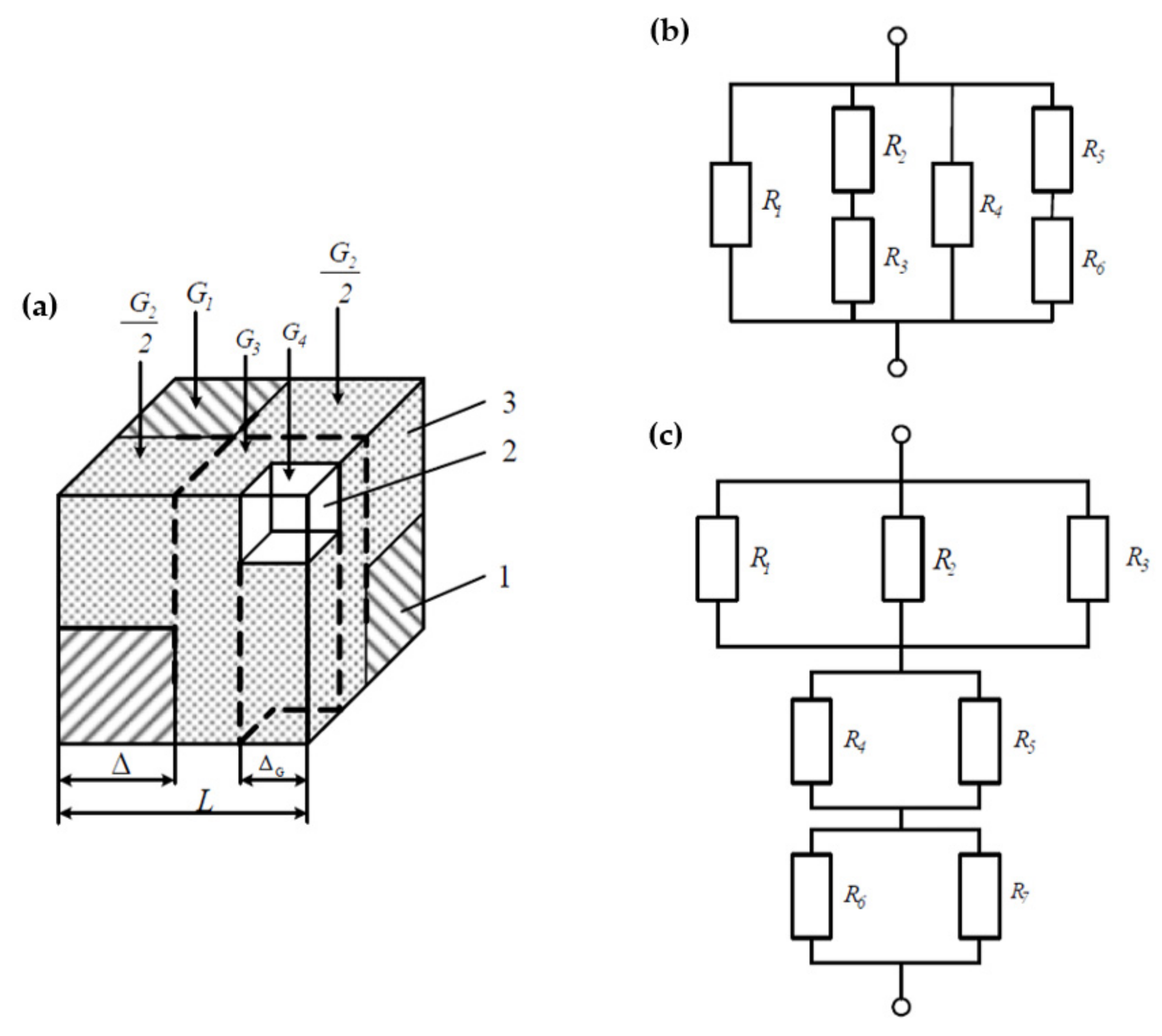
In the case of closed gas inclusions, the model of the real structure of a moist porous material constructed taking into account the assumptions of the theory of generalized conductivity [
5] for the eighth part of the unit cell has the form shown in
Figure 1a. The total heat flux
, consisting of interconnected fluxes
, flowing through unit cell individual elements, the total area of which
, passes through the considered unit cell parallel to its lateral faces.
Let us consider the derivation of the dependence for determining the effective thermal conductivity
of a given unit cell when it is divided by infinitely thin adiabatic planes parallel to the heat flux
and impenetrable for individual components of the heat flux (
). As a result, the volume of the unit cell was broken into 8 homogeneous elements. The thermal resistance of the
i-th element is calculated by the formula
where
—length of the heat flux (height) of the
i-th element, m;
coefficient of thermal conductivity of the i-th element, W/(m·K);
cross-sectional area of the i-th element, m2.
The heat flux
passes through the element of the rigid skeleton having a length
, transverse cross-section
, and thermal conductivity
. According to Formula (1), we have the resistance
The heat flux
with a cross section
passes through the liquid and solid components with resistances
The heat flux
with a cross section
passes only through the liquid component with resistance
Finally, the heat flux
with a cross section
passes through the gas and liquid components with resistances
The connection diagram of the unit cell resistances is shown in
Figure 1b. In this case, the total thermal resistance of the unit cell
is determined as follows:
The total thermal resistance of an element of the volume
, filled with a homogeneous substance with thermal conductivity
, is found by the formula
Upon rewriting Formula (6) taking into account (7) and (2)–(5), after simple transformations, we obtain the dependence for determining the effective thermal conductivity of a three-component system with the gas component in the form of an isolated inclusion, with adiabatic division of the unit cell
where
.
In what follows, we will show the derivation of the equation for determining the effective thermal conductivity of the same three-component system with the isothermal division of the unit cell. We divide the unit cell, shown in
Figure 1a, by two planes perpendicular to the total heat flux into three layers of different thicknesses. The thickness of the first (upper) layer is
, the second (middle) layer is
, and the third (lower) layer is
. In each layer, the components are separated by adiabatic planes parallel to the general heat flux. As a result, the first layer consists of three elements, and the second and third layers of two elements, the thermal resistance of which can be determined by Formula (1).
For the first layer, we obtain the following resistances:
For the second layer, we have the following two resistances:
We also have two resistances for the third layer:
The connection diagram of thermal resistances of the three layers of a unit cell is shown in
Figure 1c. For such a scheme, the total thermal resistance of the unit cell
can be written as follows:
After substituting the resistances determined by formulas (9)–(11) into relation (12) and taking into account Formula (7), we obtain a dependence for determining the effective thermal conductivity
of the three-component system with isothermal division of the unit cell shown in
Figure 1a
where, as in Formula (8),
.
With a known volumetric concentration of the solid skeleton
, the value of
c can be determined by formula [
10]
On the other hand, if the value of c is known, then one can determine
[
10]
as well as the porosity of the material
As for the value of
, it is necessary to show the scheme for its calculation. With a known value of
and a wetting angle
, we determine the boundary value of the pore moisture content
using the results of [
7]. If the contact angle is unknown, then based on the data for quartz sand, sandstone [
9], and polymer [
8], it can be taken as equal to 45°. For example, using Formula (6) of [
7], for
and
c = 0.5, we obtain
. Then the volumetric concentration of closed gas inclusions in the pores is equal to
and, respectively, in the material
. By definition,
. With a decrease in the contact angle
, the value of
increases. Thus, for
and
, we have
. Note that the inequality
holds for
and
.
Calculations by formulas (8) and (13) give the lower and upper estimates of the effective thermal conductivity of a moist porous material, and its final value should be determined as the arithmetic mean .
In what follows, we consider the derivation of the formula for a system whose gas and liquid components are continuously distributed, interpenetrating each other. The pore moisture content
is between two boundary values
. In this range, according to the percolation theory [
5], two independent approaches are possible. In the first approach, the structure of the gas component is specified as the main one, whereas in the other, the structure of the liquid component is specified.
3. Thermal Conductivity of a Three-Component System with a Specified Structure of the Gas Component
This case in the form of the eighth part of the unit cell is shown in
Figure 2. When deriving the dependences, it is assumed that the size
found for a closed gas inclusion in the center of the cell does not change (
) with an increase in the volume concentration of gas
. Then, the increase in
leads to an increase only in the size
of the gas channels connecting the gas inclusion of size
in the center of the cells. In this case, the condition
must be met.
After the division of the unit cell shown in
Figure 2 with adiabatic planes and the implementation of the procedure used to find Formula (8), a dependence is obtained to determine the effective thermal conductivity
(lower estimate) of the three-component system with a continuous inclusion of the gas component
where
.
After dividing the same unit cell by isothermal planes into four layers and determining the thermal resistances of each layer, and after transformations, as in the derivation of Formula (13), we obtain the dependence for determining the effective thermal conductivity
(upper estimate) of the three-component system under consideration
where, as in (17),
.
Let us determine the value of
cm at a known volumetric gas concentration
.
Figure 2 shows that the volume of the pore channels is
. On the other hand, the same volume is equal to
, where
is the total volume of gas in the cell. After dividing these volumes by the cell volume
, we come to the equation
solving which we find the value of
.
According to Formula (19), at
we have
. This indicates the disappearance of gas channels connecting the gas inclusions in the center of the cells. The range of formulas (8) and (13) is obtained by formulas (17) and (18). In this case, formulas (17) and (18) provide a transition from a structure with a continuous gas phase (
Figure 2) to a structure with isolated gas inclusions (
Figure 1).
4. Thermal Conductivity of a Three-Component System with a Specified Structure of the Liquid Component
In this case, the unit cell has the form shown in
Figure 3. For the cell under consideration, the formulas for calculating the lower
and upper
estimates were obtained for the evaluation of the effective thermal conductivity of moist capillary-porous materials using the method described above.
After dividing the unit cell (
Figure 3) with adiabatic planes, we obtain
where
The dependence obtained by dividing the same unit cell with isothermal planes has the form:
where, as in (20),
The
value is related to the volume of the liquid at the rod node of the solid skeleton of the unit cell
. The moisture content of the material in the rod node
is determined from the condition that the pore moisture content is equal to the lower boundary value
. Then, we obtain
.
Figure 3 shows that the volume of the liquid at the node is
. By dividing the left and right sides of this expression by the volume of the unit cell
and denoting
, we obtain the cubic equation
solving which we obtain the physically justified root
(with a known value
) and, therefore, the value
.
In accordance with the theory of percolation [
5], we assume that with an increase in the total moisture content of the material
, the moisture content in the network node
does not change (
). With a known difference
, the
value can be determined. As shown in
Figure 3, the volume of liquid
distributed over the length
of the three rods of the unit cell is equal to
. By dividing this equality by the cell volume
, we obtain a quadratic equation with an unknown
the positive root of which gives the desired value of
.
If after the application of Formula (23), it turns out that , then it is necessary to use formulas (17) and (18) to determine the thermal conductivity of the material.
From Formula (23) it follows that at
we obtain
. Then Formulas (20) and (21) are transformed to the forms of (23) and (28), presented in [
7], which describe the structure of a three-component system with isolated liquid inclusions. Thus, Formulas (20) and (21) provide a smooth transition from the structure with a continuous liquid component to a structure with isolated inclusions of liquid and vice versa. In addition, in the absence of a liquid component, these formulas take the form of the known dependences formulated for a system with two interpenetrating components [
5] at the adiabatic
and isothermal
division of a unit cell. Here,
.
5. Limitations of the Application of the Formulas
To determine limitations of the application of the formulas obtained herein, we use the dependence of the pore moisture content
on the boundary values
and
in the following form:
where
K is a coefficient varying within the lower
and upper
boundaries. It is obvious that
.
According to the assumptions made, formulas (20) and (21) can be used for determining the values of the coefficient from the lower boundary of to some , for which . It is easy to assume that the results of calculating the thermal conductivity by formulas (20) and (21) will differ from the results obtained by formulas (17) and (18), since the former neglect the presence of the gas inclusion in the center of the unit cell, and the latter does not take into account the uneven distribution of the liquid component. It was of interest to determine the value of , up to which formulas (20) and (21) can be used, and at the same time compare the results obtained by formulas (20), (21) and (17), (18) for this . A similar comparison was made for other values from the range . It required doing calculations according to the indicated formulas.
These calculations were performed using a three-component system with the constant volume concentration of the solid skeleton
(
,
) and thermal conductivity
W/(m·K). The thermal conductivity of the gas and liquid components,
W/(m·K), and
W/(m·K), respectively, was also constant. Concentrations of the gas and liquid components varied depending on the moisture content of the system. The wetting angle
θ based on the data from [
8,
9] was taken as equal to 45°.
First, let us determine the boundary values of the moisture content with respect to
and
at a wetting angle
According to [
8]
Then we calculate the moisture content in the cell node . The value was found from the solution of the cubic Equation (22). Having given from the range , using Equation (26), we calculate the pore moisture content , by which we determine the concentration of the liquid component , and then, using Equation (23), we determine . Using the method of successive approximations, we selected , at which (accuracy 0.0001). Concentrations m3 = 0.4288 and were found for this . Further, using formulas (20) and (21), the thermal conductivities λ W/(m·K) and W/(m·K) were determined, and the estimate of the effective thermal conductivity W/(m·K) of the three-component system was calculated.
At the same concentrations of the components, the corresponding thermal conductivities W/(m·K), W/(m·K), and W/(m·K) were found by formulas (17) and (18). The last result for exceeded the previous one by 1.77%. The smallest increase by 1.1% was observed at .52, and the largest was at the lower border of , amounting to 9.68%. At the upper border, , the relative difference was 2.22%. We came to similar results after performing calculations for other values of the parameters с and θ. From a physical point of view, for , more accurate results should be given by formulas (20) and (21). Formulas (17) and (18) can be applied in a rather narrow range of from to .
6. Preparation of Initial Data for the Calculation
To perform calculations using the obtained formulas, it is necessary to know the volume concentrations and thermal conductivities of the components. With the known apparent density and moisture content of the material, as well as the density of the solid skeleton , which can be determined using pycnometry, the concentrations of the components are determined quite simply:, and .
The thermal conductivity of water (liquid component)
W/(m·K) is easy to find by the formula obtained by approximating the data [
11]
where
is temperature in °C.
The thermal conductivity of vapor–air mixture
(gas component) is the sum of the thermal conductivity of dry air
and thermal conductivity of vapor
generated by diffusion transfer of vapor in the pore space. The first parameter is determined by formula [
6]
The
value is determined by formula [
5], based on the Krisher dependence [
12],
where
—diffusion coefficient of water vapor in still air, m2/s;
—coefficient of resistance to vapor diffusion through the pore space;
—molecular weight of water vapor, kg/mol;
—universal gas constant, J/(mol·K);
—temperature of water vapor, K;
—total pressure of water vapor and air, Pa;
—partial pressure of water vapor, Pa;
—specific heat of water vaporization at the temperature t, J/kg.
When determining the diffusion coefficient of water vapor, the formula proposed by
R. Schirmer in 1938 is usually used [
12,
13]:
The derivative
can be determined using reference data or by formula [
12]
The dependence of the specific heat of water vaporization on temperature after approximation of the reference data has the form:
The vapor diffusion resistance coefficient
for a continuous gas component (,
), according to [
8,
14], can be determined by the formula
where
is calculated from Formula (14) after substitution of the solid component concentration
with the gas component concentration
. For closed gas inclusions (
Figure 1,
)
μ = 1.0.
In the first approximation, the thermal conductivity of the solid component can be determined using Equations (24) and (25), in which and are taken to be equal to the thermal conductivity of dry material , and then the values of the thermal conductivity of the solid skeleton are found by the method of iteration for the adiabatic and isothermal division of the unit cell. The average value is taken for subsequent calculations.
Thus, to calculate the thermal conductivity of a moist material, a minimum amount of experimental data for a dry material is required, i.e., the apparent density of the material and its skeleton density , as well as the thermal conductivity . The rest of the initial data can be determined by calculations.
7. Calculation Examples
The features of calculating the effective thermal conductivity of a moist capillary-porous material according to the formulas will be demonstrated by examples using experimental data for clay bricks presented in
Table 1, obtained by us, and published in [
15]. However, there is no information about the skeleton density
in [
15].
To determine the density
we constructed a linear regression equation based on data from eight pairs of values of
and
for clay bricks with apparent density
from 1530 to 2120 kg/m
3The above equation based on the
F (Fisher) test is effective with a confidence level of 0.95. The thermal conductivity of clay bricks depends on a large number of factors, and its measured values in the
n-element test show a significant dispersion characterized by the standard deviation
. Based on the data of a representative test obtained on moist ceramic samples with apparent density
from 1550 to 1850 kg/m
3 [
16], the coefficient of variation
(the ratio of
s to the sample mean
) was 0.16 (16%). According to our data obtained for nine dry samples with apparent density
ρ from 1510 to 1900kg/m
3, the coefficient of variation was 0.073.
Example 1. For three brick samples, the following average values were determined: the apparent density
kg/m3, the density of the solid skeleton
kg/m3 according to pycnometry, and the thermal conductivity of material in the dry state,
W/(m∙K), and in the water saturated state, (
)
W/(m∙K). The thermal conductivity was measured by a stationary method at a temperature of 20 °C. The contact angle
was taken as equal to 45°. The same temperature and angle θ values were also used in the remaining examples.
In this case, we have volumetric concentration of the solid component , at which, according to (14), and porosity ; concentration of liquid and gas components; and boundary values and , and and , calculated by formulas (27), (28), and (26). The moisture content in the cell node , which from the solution of Equation (22) was worked out. Then, by solving Equation (23), was determined. From the inequality it follows that it is necessary to use formulas (20) and (21) for calculating the thermal conductivity. As already noted, this can be confirmed using the coefficient determined by Formula (26). At , we have the actual coefficient , whose value does not exceed , which determines the upper boundary of applicability of Formulas (20) and (21), and which is found from the condition To perform calculations using these formulas, it is necessary to determine the values of the thermal conductivities of the components at the assumed temperature of 20 °C. The thermal conductivity of the solid component was determined using formulas (24) and (25), in which and were equated to W/(m∙K). Then the values W/(m·K) and W/(m·K) were found by the method of successive approximations to calculate the accepted W/(m·K).
Before determining the thermal conductivity of the gas component
, it was worked out that its concentration
exceeds the gas concentration in the center of the unit cell
; therefore, the gas component is continuous (
Figure 2). In this case, the vapor diffusion resistance coefficient
is determined by Formula (35). Using Equation (31), the thermal conductivity of the diffusing vapor
W/(m∙K) was calculated. According to Formula (30), the thermal conductivity of dry air is equal to
W/(m∙K). The thermal conductivity of the gas component (vapor–air mixture) is found by summation [
5]
W/(m∙K).
The thermal conductivity of the liquid component, calculated by Formula (29), is equal to W/(m∙K).
After completing the initial data, the thermal conductivity W/(m∙K) was calculated according to Formula (20) and W/(m∙K) according to Formula (21), and the effective thermal conductivity of the material was found W/(m∙K), which turned out to be 5.53% lower than the experimental value.
Example 2. According to [
15]
, a clay brick with apparent density kg/m3 had the thermal conductivity
W/(m∙K) in a dry state and
W/(m∙K) in a water-saturated state (
). The density of the skeleton of the material
kg/m3 was determined by Formula (36). Further, as in example 1, the initial data necessary for the calculation were established, and according to formulas (20) and (21), the lower W/(m∙K) and upper W/(m∙K) estimates of the thermal conductivity of the material were determined. The accepted estimate of the effective thermal conductivity of the material W/(m∙K) is 9.2% lower than the experimental value.
Example 3. According to [
15]
, for a clay brick we have kg/m3,
W/(m∙K), and
W/(m∙K) at
(water saturation). By Formula (36),
kg/m3. On the basis of this information, as before, the initial data were prepared by calculations using formulas (20) and (21):
W/(m∙K), and
W/(m∙K). The average value
W/(m∙K), taken as an estimate of the effective thermal conductivity of the material, turned out to be 8.25% lower than the experimental value
W/(m∙K). As is shown in Table 1, the deviations of the calculated values of λ from the experimental ones observed in these examples are practically two times less than the mentioned coefficient of variation
(relative standard deviation). Therefore, there is reason to believe that the proposed formulas with reliable experimental data are capable of predicting the thermal conductivity of moist capillary-porous wall materials with sufficient accuracy. 8. Conclusions
Several equations were constructed to determine the effective thermal conductivity of moist capillary-porous materials, the pore moisture content of which, with free liquid absorption, may vary from hygroscopic level to full saturation. These materials were considered heterogeneous three-component systems consisting of a solid skeleton, gas (vapor–air mixture), and liquid (water). Thermal conductivities and volumetric concentrations of all components were simultaneously taken into account, and the methods of the theory of generalized conductivity were used for the analysis of heat transfer in such systems. The structure of the solid skeleton was modeled by an ordered structure of identical unit cells of the simplest, cubic shape.
Changes in the binary structure of interconnected liquid and gas components were analyzed as the pores were filled with liquid. First, liquid inclusions, then continuous components of liquid and gas, and, finally, closed gas inclusions were considered. The geometric model of the three-component unit cell of each of these structures was described according to the theory of percolation, and for each unit cell, equations were constructed to determine its thermal conductivity during adiabatic and isothermal division. Moreover, limitations of the application of these equations were determined.
From a physical and practical point of view, it is expedient, first of all, to use formulas (20) and (21), which provide a smooth transition from a structure with a continuous liquid component to a structure with isolated liquid inclusions and vice versa, and allow determination of the thermal conductivity of a moist material up to the state of free saturation with water. The scope and method of preparing preliminary data for calculations were explained. The details of the calculations according to the proposed formulas were demonstrated by examples using experimental data for clay bricks. It was found that formulas (20) and (21) are capable of predicting the thermal conductivity of wet capillary-porous wall materials with sufficient accuracy.
The developed methodology of calculation of thermal conductivity of moist capillary-porous materials can be useful for the sustainable design of new buildings and renovation of historic ones.


 ,
, 


