Abstract
Particulate matter has become one of the major issues in environmental sustainability, and its accurate measurement has grown in importance recently. Low-cost sensors (LCS) have been widely used to measure particulate concentration, but concerns about their accuracy remain. Previous research has shown that LCS data can be successfully calibrated using various machine learning algorithms. In this study, for better calibration, dynamic weight was introduced to the loss function of the LSTM model to amplify the loss, especially in a specific band. Our results showed that the dynamically weighted loss function resulted in better calibration in the specific band, where the model accepts the loss more sensitively than outside of the band. It was also confirmed that the dynamically weighted loss function can improve the calibration of the LSTM model in terms of both overall performance and local performance in bands. In a test case, the overall calibration performance was improved by about 12.57%, from 3.50 to 3.06, in terms of RMSE. The local calibration performance in the band improved from 4.25 to 3.77. Such improvements were achieved by varying coefficients of the dynamic weight. The results from different bands also indicated that having more data in a band will guarantee better improvement.
1. Introduction
Particulate matter has become one of the world’s major air pollution issues, and its impact on people and society has been widely investigated and highlighted. Particulate matter affects public health in both the short and long term, causing respiratory and cardiovascular diseases [1]. High concentrations of particulate matter have a wide range of adverse effects. In October 2013, the International Cancer Institute (IARC) under the World Health Organization (WHO) classified particulate matter as a Group 1 carcinogen, similar to asbestos and benzene, which have serious adverse effects on humans. WHO announced that, in 2014 alone, seven million people died earlier than expected due to particulate matter [2]. WHO has suggested as a guideline that an air quality of PM2.5 should be maintained at an annual average of 10 μg/m3 and a daily average of 24 μg/m3 or less, and many countries, including South Korea, follow such criteria. As such, checking the concentration of particulate matter has already become a daily routine and even publics adjust their expenditures to reduce the particulate matter emissions [3].
To deliver more accurate information about ambient concentrations of particulate matter to the public, the government has established measuring stations with high-cost equipment [4]. The Korean Ministry of Environment has adopted the beta-ray absorption method and the gravimetric method as standard approaches for measuring particulate matter in the atmosphere. In this study, these methods are called the standard method of the government (SMG). The beta-ray absorption method measures the mass concentration of sampled particulate matter using the change in beta-ray intensity when it is transmitted through the sample. The gravimetric method directly determines the mass of the ambient particulate matter by measuring the difference in weight of a filter before and after sampling [5]. These standard methods demand skilled operators, large space and high investment, because they involve sensitive operation and management issues.
Optic sensors used with the infrared ray scattering method are low-cost sensors (LCS) and can complement the SMG measurement temporally and spatially [6,7]. Despite their relatively low reliability and accuracy compared to the SMG, LCS are widely utilized for measurement because they offer convenient, economical, and practical usage. In particular, LCS can improve their measurements with high temporal and spatial resolution due to their low cost to install [8]. Most indoor air purifiers contain LCS to measure indoor air quality, which has different characteristics than the outdoor atmosphere. These LCS can be used to not only measure air pollution, but also to detect the particulate matter in other domains such as wildfires [9], marine monitoring [10], and building constructions [11].
2. Literature Review
2.1. The Limitation of Low-Cost Sensors Compared to the Standard Methods of the Government
LCS performance can be distorted by various factors that become reasons for their inaccuracy [12,13]. As LCS do not sample and dry the particulate matter, microscopic droplets can distort the scattering of the infrared rays [14]. The absorption of infrared rays by humid air lowers sensor performance [15]. The data quality is also diminished in extreme conditions such as sand storms [16]. It is also sensitive to local events such as wind gusts and cigarette smoke, so that data measured by LCS is sometimes inaccurate in high temporal resolution [17]. When conducting this study, we noted that, for some LCS with suction fans, dust covered the suction hole forming a dense web-like structure, which strongly distorted the measurement.
Although manufacturers calibrate their error, the LCS usually overestimate the concentration of particulate matter because of differences between the actual environment and the environment in which pre-calibration was performed. Sometimes, the pre-calibration does not consider the distorting factors [18]. Some recalibration models that contain regional meteorological conditions have been studied [19]. On-site recalibration is required in the actual field or environment where LCS are placed [13,20,21].
Since LCS are more frequently used in living areas, more caution has recently been given to their accuracy and calibration. Studies have investigated their calibration considering the error-causing factors. Liu et al. [22] developed a package for LCS used to measure PM2.5 emitted by traffic on a road. They improved the reliability of measurement by calibrating with meteorological factors such as temperature and humidity. Zheng et al. [23] investigated their performance under in-field conditions and suggested that nonlinear calibration using weather factors such as relative humidity can improve the sensor performance.
2.2. Deep Learning Applications for Calibrating Low-Cost Sensors
The calibration methods of LCS can be categorized into physical mechanism-based models, parametric models, and nonparametric models such as machine learning algorithms [24]. The mechanism-based models incorporate the relative humidity for calibration because it distorts the optical measurement of LCS. The parametric models, such as regression models, are easy to apply but make it difficult to capture the nonlinear relationship between various factors that affect on-site LCS.
Many previous studies have adopted machine learning algorithms for calibration because of their high performance solving nonlinear relationships. Wang et al. [25] showed that the random forest model performed better than the linear regression model for calibrating LCS. Johnson et al. [26] showed that the gradient boosting model using meteorological data as input could significantly improve the calibration of low-cost sensors compared with the linear regression method. Loh and Choi [27] calibrated sensors with SVM, k-nearest neighbors, random forest, and extreme gradient boosting algorithms using a web query of government-approved data to calibrate LCS. Wang et al. [28] verified the powerful calibrating capacity of machine learning algorithms by comparing multiple linear regression, support vector regression, and random forest regression models. The latest machine learning algorithms have been successfully applied to calibrate LCS [29]. Rengasamy et al. [30] applied a dynamically weighted loss function to improve the performance of deep learning models without modifying their architecture.
2.3. Band-Sensitive Calibration for Low-Cost Sensors
The public perception of air pollution is often more influenced by the level of bad air quality, shown in Table 1, than the actual value of measured concentration itself, since they are more familiar with the levels identified in the government regulations [31,32]. Concentrations related to the level of air quality are carefully determined to evaluate the potential health effect to public [33]. The Korean government has adopted four levels of PM2.5, as shown in Table 1. Different regulations and enforcements are applied to different levels. Accordingly, the particulate matter concentration near the upper or lower limits of individual levels require more-precise calibration than any other values. In conditions where the amount of the particulate matter is a little distance away from the limits, people are less sensitive to error in measurement. As a result, we argue that more-precise calibration should be conducted at the limits of two levels, which are designated “Bad” and “Very bad” in Korea, as shown in Table 1.

Table 1.
The four levels of PM2.5 and their corresponding concentration in South Korea.
The novel idea in this research is to assign a different importance to errors in the machine learning training process, according to the concentration of particulate matter. This will make errors occurring in a specific band of concentration more sensitive to training. The contribution of this research is to suggest a methodology to improve calibration by giving more weights to errors in specific concentration bands than those outside the band. Users can set their band of interest, which should then be trained with a relatively high importance in a machine learning model, so that the model responds more sensitively to errors within the band. For example, those who have a stake in a specific particulate matter concentration can set a band around that concentration.
In locations such as nurseries and kindergartens, managing indoor particulate matters is an important issue to protect the health of babies and children. That is, especially in Korea, why those locations try to maintain indoor particulate matter below a level of “Bad”, i.e., Level III, and why their managers are more concerned with the concentrations near the limits of Levels II and III. This study is thus designed to provide better calibration near those limits for their more-accurate estimation by assigning specially devised weights to the concentrations near the limits. As an illustration, in-field concentrations of PM2.5 were measured using an LCS at the same location where an SMG was being operated. The measured data from the LCS were calibrated to the data of the SMG using an LSTM model. During training by the LSTM model for calibration, dynamic weight was applied to the loss function to make a certain band more sensitive to error.
3. Methodology
A recurrent neural network (RNN) is suitable for training sequences such as time series data because of its characteristic of updating the weights of neurons by recursively referencing the previous state of the output layer. However, a vanilla RNN model is known to have limited long-term dependency. Hochreiter and Schmidhuber [34] proposed the long short-term memory (LSTM) model which, by designing a neural network structure, can explicitly overcome the long-term dependency problem. The LSTM model conveys a current input sequence to each gate to control how much of the previous information should be conserved, and how much of the current information should be accepted.
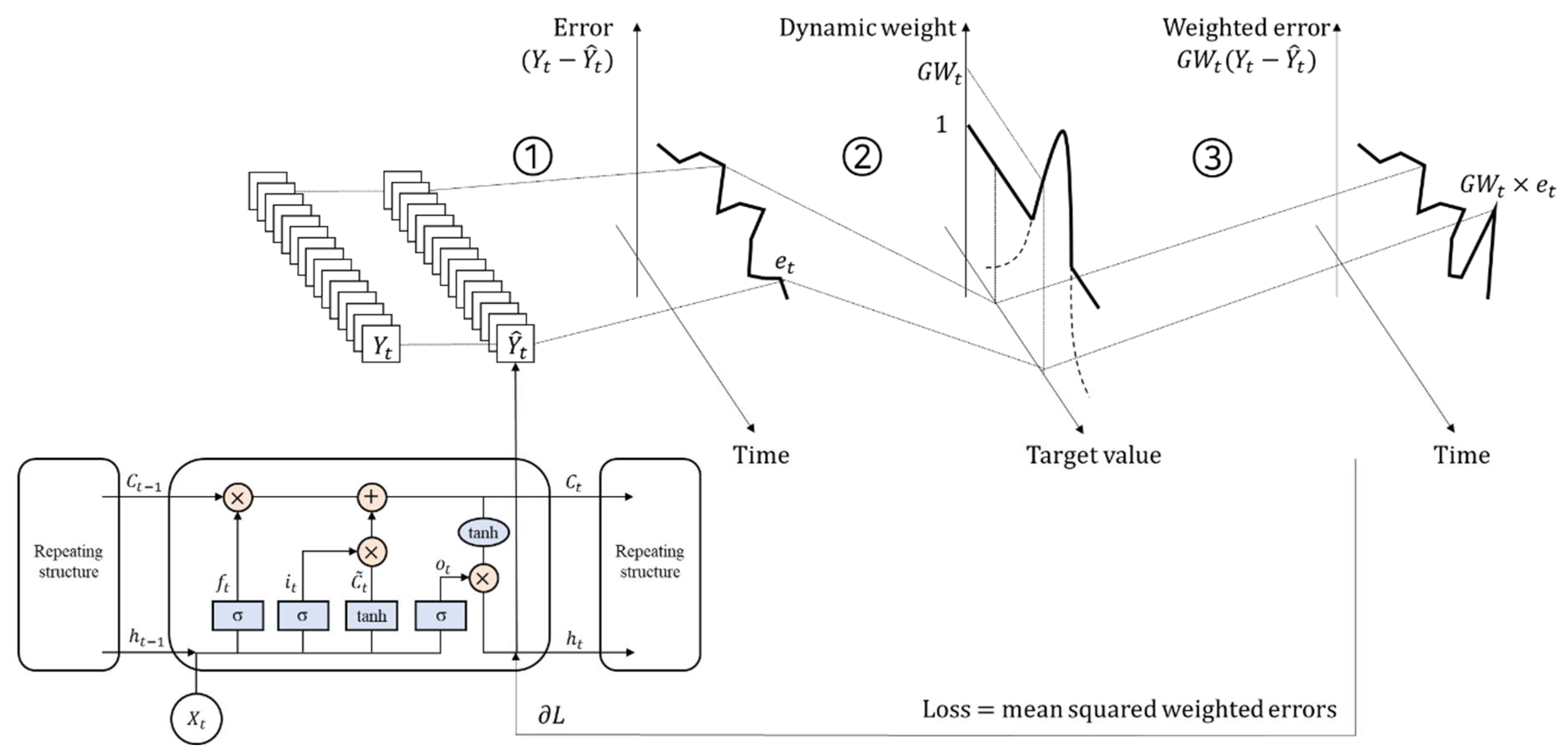
As illustrated in Figure 1, the LSTM model was introduced with a dynamic weight as follows. The architecture of the LSTM model was identical to that of the original study [34]. However, errors are amplified in a band of interest in below process after feedforward propagation.
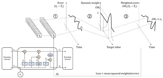
Figure 1.
The concept of the LSTM model with a dynamic weight. After feedforward propagation, ① the errors are calculated from outputs of the LSTM and target values; ② some errors are amplified according to their dynamic weight; and ③ the loss is calculated by loss function, i.e., the MSE in this study, and the gradient is back-propagated to update weights and biases in the LSTM model.
- The errors are calculated from the outputs of the LSTM model and target values;
- Errors occurred in the band of interest are amplified using their dynamic weight;
- The loss is calculated by loss function, i.e., the mean square error (MSE) in this study, and the gradient is back-propagated to update weights and biases in the LSTM model.
The mean squared error (MSE) in Equation (1) is a common loss function for time series prediction and regression tasks, including calibration with the LSTM model. As it is literally the mean of squared error between the target and prediction, it indicates that there are no more- or less-important errors in training, regardless of the target value.
is from SGM and is output from LSTM model
where a, b and c are coefficients of a Gaussian function . is the length of target variable and its prediction .
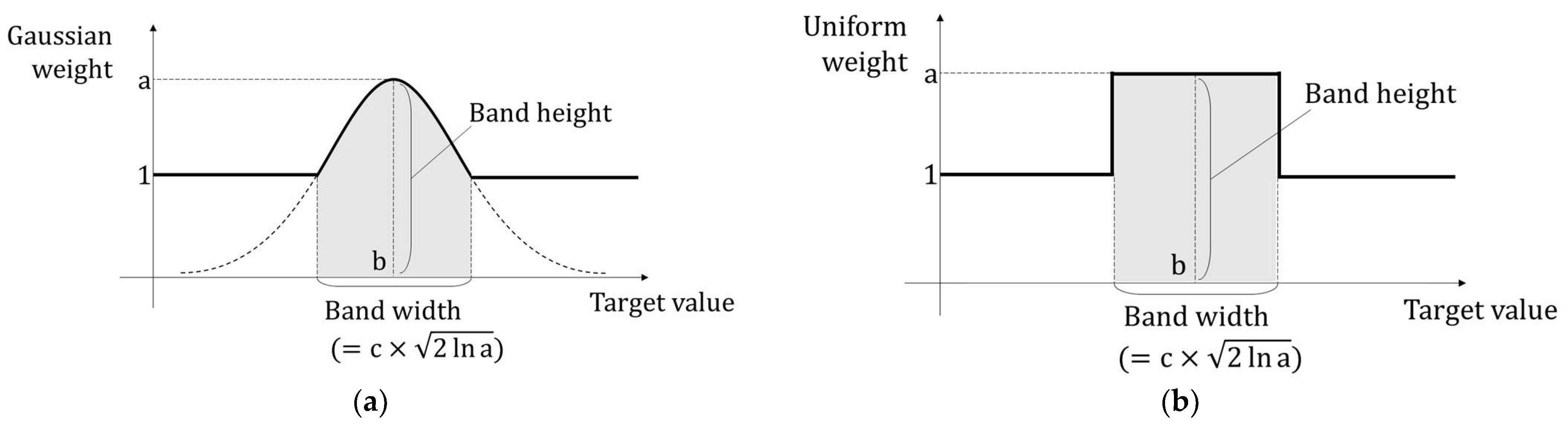
As shown in Figure 1 and Equations (2) and (4), we introduced Gaussian weights to MSE. The weight function is a symmetric shape with a peak. It smoothly decreases from the peak, especially slowly just around the peak. Simple Gaussian weight leads the LSTM model to ignore errors at very low or high target values because the Gaussian function converges to zero at the tails. As shown in Equation (4), a band determined by the coefficients of Gaussian function was introduced to overcome this ignorance. The Gaussian coefficient b determines the center of a band. The coefficients of a and c control the band width, which determines the boundary where the Gaussian weight is not less than one. Additionally, a uniformly weighted MSE in Equations (3) and (5) with the same height and width as the Gaussian case was also used for comparison. Figure 2 shows the weight functions that were introduced.
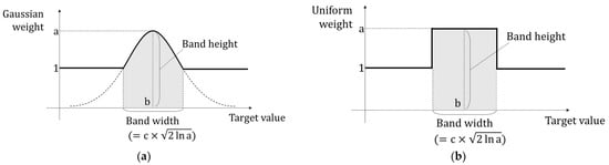
Figure 2.
Two types of weights given to the loss function of the LSTM models: (a) Gaussian weight, and (b) uniform weight.
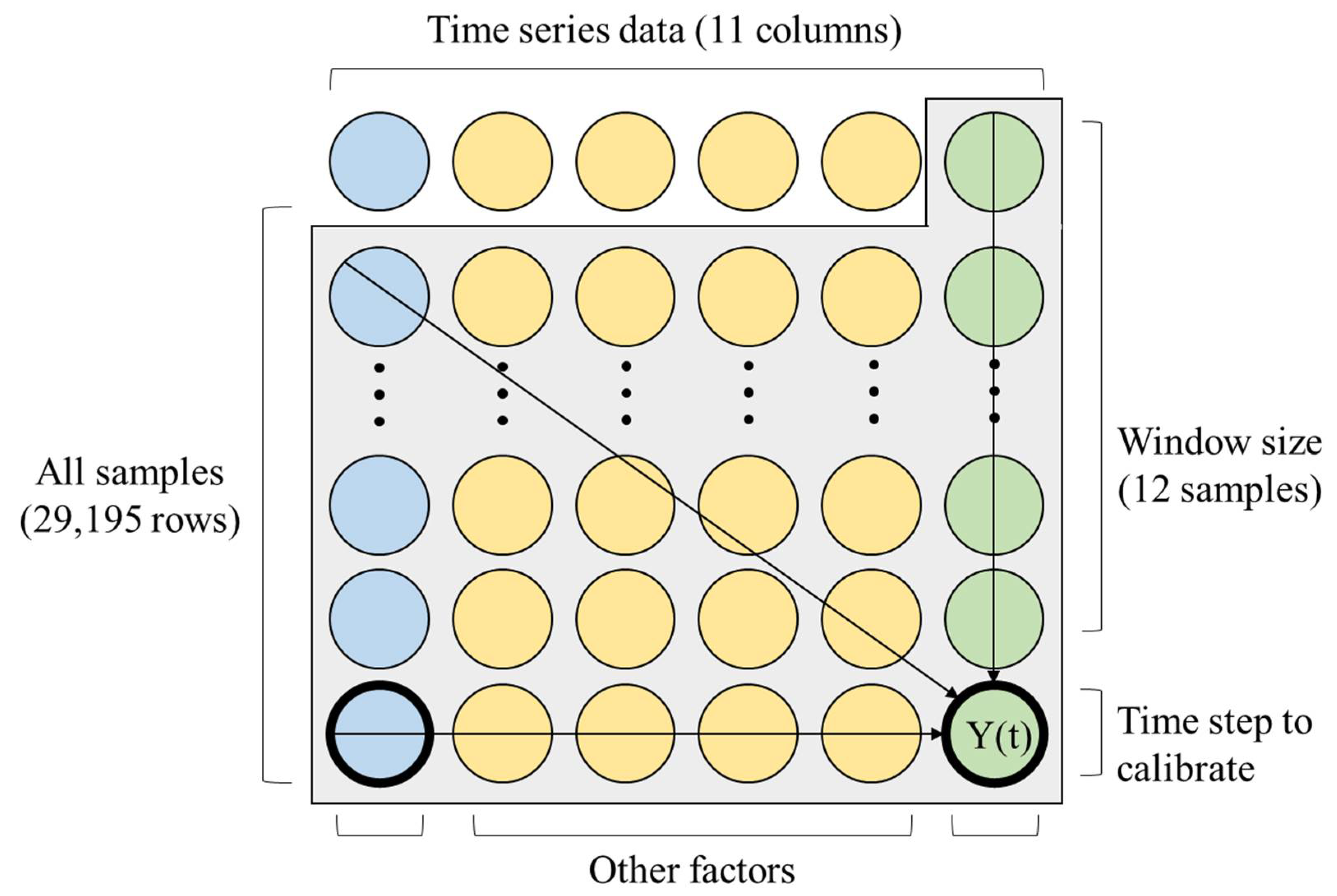
Figure 3 shows the input and output structure trained to the LSTM model. The blue, yellow, and green circles indicate the input data. The green circles also indicate the output target value. At each step, a set of rows in the gray frame was shifted into the model, just to convey the input sequences and target value to the LSTM model. The window-sized length of the input sequences in the grey frame was conveyed to train the model at the same time. The time step for the output could be set to one because calibration does not require multi-dimensional outputs. The task given to the LSTM model was calibration, which coercively adjusts the measurement from the LCS, indicated by the bold circle in the left bottom corner, to the target value from a reference measurement, the bold circle in the right bottom corner in Figure 3. Note that the output of the LSTM model is not a future value, but the present value at the same time.
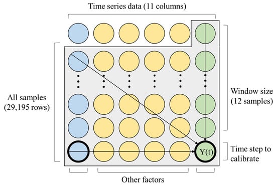
Figure 3.
The task for the LSTM model and the structure of the input sequence and output.
The calibration performance of the LSTM model was evaluated by root mean squared error (RMSE) in Equation (6) and mean absolute percentage error (MAPE) in Equation (7) to complement each other. RMSE can be considered an error but it is scale-dependent on the target value. MAPE converts the error to percentage to overcome the disadvantage of the RMSE, but it is exaggerated at low target values. The calibration performance can be more-effectively evaluated by calculating both metrics.
4. Experimental Setup and Preprocessing
4.1. Experimental Setup and Data Collection
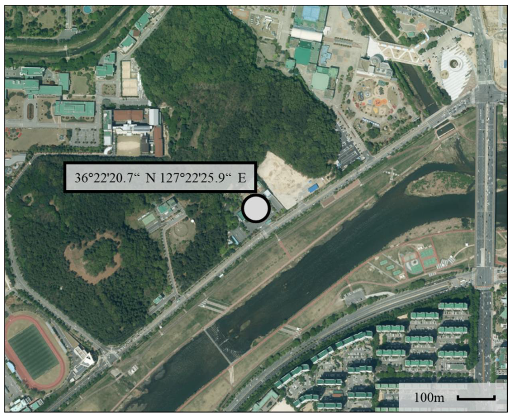
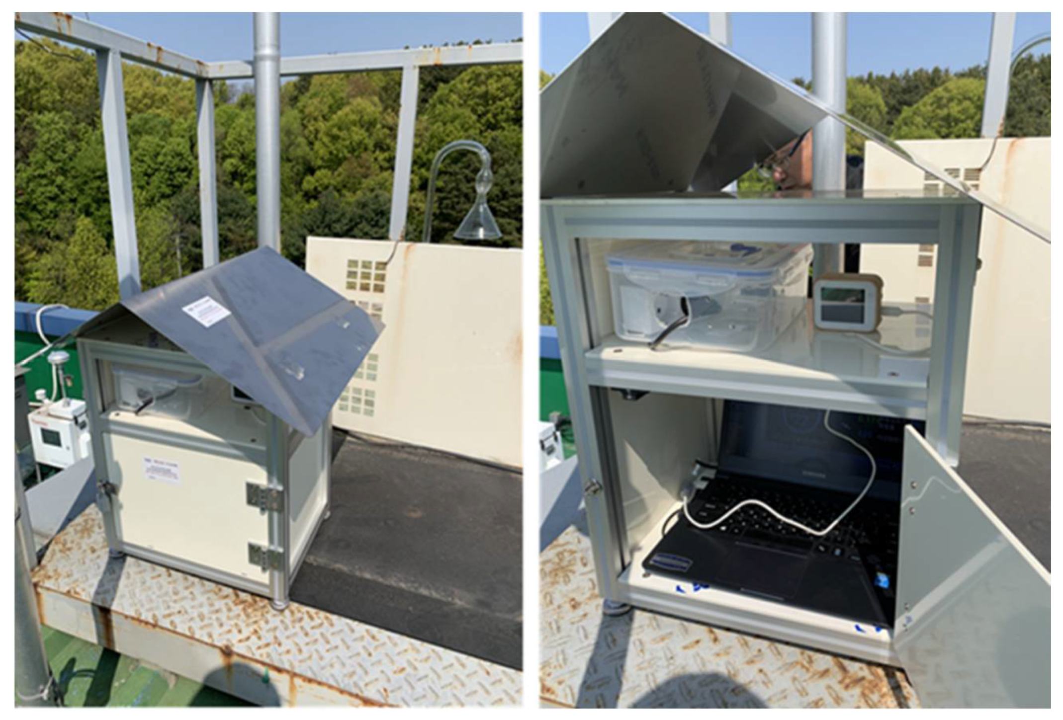
Figure 4 and Figure 5 show the experimental setup at the Daejeon Institute for Health and Environment where the concentration of PM2.5 was measured by the SMG, using the beta-ray absorption method and gravimetric method, for public use in Daejeon city. A commercial LCS product containing a PMS 7003M manufactured by Plantower [35] was installed next to the air sampler of the equipment. The experimental installation required a roof to protect the sensor from rainfall and direct sunlight. The sensor was placed at the height of the air sampler to maintain a distance to avoid heat interference. There was no interruption of air flow near the sensor.
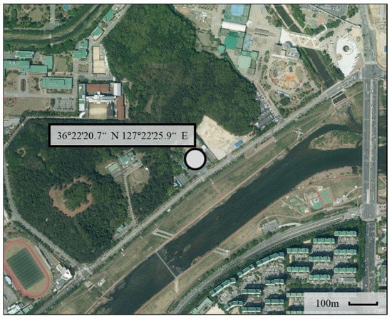
Figure 4.
The research site used to measure data with the low-cost sensor and the beta-ray sensor.
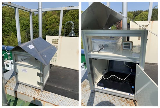
Figure 5.
The experimental setup at the research site. The low-cost sensor is placed at the same height as the sampler of beta-ray sensor. The roof blocks direct sunlight and rainfall.
PM2.5 was measured every 10 s from May 2020 to August 2020 using the LCS with the PMS 7003M. The same PM2.5 was also measured by the SMG using a 5014i Beta Continuous Ambient Particulate Monitor from Thermo Fisher Scientific, Waltham, MA, USA [36]. The SMG measured every 5 min and its measurement was used as the target value in the LSTM model. The data from the LCS was averaged every 5 min to match the target values of the SMG. A total of 29,195 observations were used as the input sequence for the LSTM model.
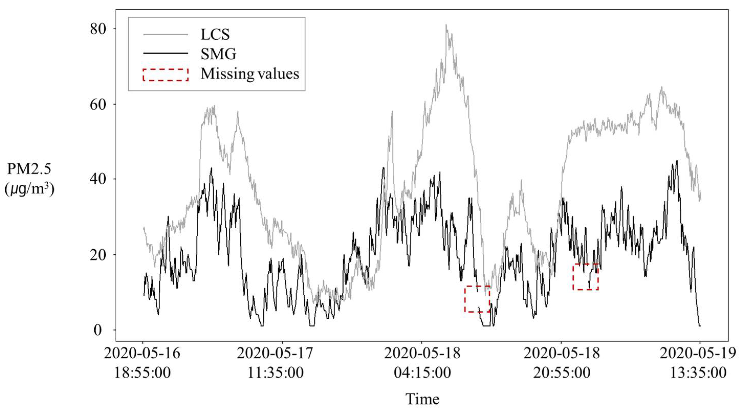
Figure 6 shows the actual measurements by the LCS in gray and those by the SMG in black. Both measurements follow same trend but an overestimation is observed in the LCS measurement. Figure 7 describes the distribution of collected data using a histogram. The histogram shows positive skewness with a right tail.
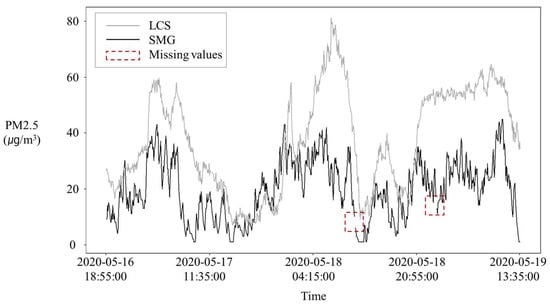
Figure 6.
The example of measurement. The plots in gray and black represent the measurements by the LCS and SMG, respectively.
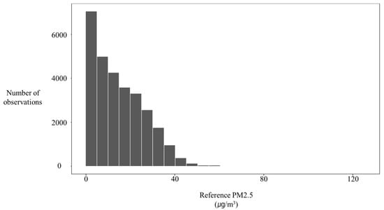
Figure 7.
The bar histogram of collected PM2.5 concentrations. (The histogram shows positive skewness with a right tail.)
Previous studies [23,25,26,27,28] suggested that integrating other factors, including air pollutants and meteorological data, improved the calibration performance of the LSTM model. This study, therefore, included those data for our analysis. The former was obtained from Air Korea which is an agency of the Korean Ministry of Environment, while the latter was from the Korea Meteorological Administration.
4.2. Data Preprocessing
Table 2 briefly shows all the data, with statistics. The missing values were simply imputed by the last observation carried forward method because their portion was negligible to the total observations and their individual durations were not long but only short segments, as shown in Figure 6. The data was normalized using Equation (8) before being trained by LSTM as input sequences. This was carried out to convert the data of different scales to a dimensionless one. The entire body of data was split into three sets, of training, validation, and test, representing 56, 14, and 30 percent of the total observations, respectively. To conserve the time-series order and continuity, k-fold cross validation was not applied. Data preprocessing and fittings were implemented in an R environment. Training and calibration process by LSTM model were implemented in a Google Colaboratory environment.
where is input for LSTM model.
Table 2.
Description of the measured and collected data.
4.3. Training and Hyperparameter Optimization
All the LSTM models in this study, with different combinations of Gaussian coefficients and types of weight given to the loss function, were evaluated by averaging the training and test results 20 times. For example, the LSTM model with a simple MSE loss function was trained and tested 20 times, and then the performance of this model was represented by the mean of the 20 different RMSEs and MAPEs. To guarantee that all the individual models were each the best in performance, each model was trained until it achieved its best performance. The results of many iterations required at least 1200 epochs to reach the global minimum of validation loss, i.e., the best performance, and hundreds of epochs after the global minimum, overfitting, appears. Therefore, an early stopping rule was devised so that each model stopped training unless a new minimum of validation loss appeared in 50 epochs after a threshold of 1200 epochs.
To more-accurately evaluate the LSTM models of the dynamically weighted loss function, used to calibrate the LCS measurements, the three parameters (a, b and c) in Eqn. 4 were adjusted and applied to the LSTM models. Their combinations are shown in Table 3, which indicates the sections whose related results are individually discussed.
Table 3.
Experimental setup with Gaussian coefficients of the loss function.
Other hyperparameters of the LSTM model were also determined by trial and error, as shown in Table 4. It was sufficiently iterated to obtain the hyperparameters where the LSTM model achieved the best performance. The window size for the input sequence was determined to be 12, which means one hour, to reflect the short-term distorting factors. Stacking an additional layer improved the performance of the models. It was concluded that 10 hidden neurons were sufficient to learn the nonlinear relationship in the input data, while the performance of models with additional hidden neurons was poorer. The dropout technique was applied by randomly turning off 30% of the hidden neurons for each epoch to avoid overfitting.
Table 4.
The hyperparameters for LSTM models.
5. Results and Discussion
5.1. Effect of Dynamic Weight on Calibration Performance
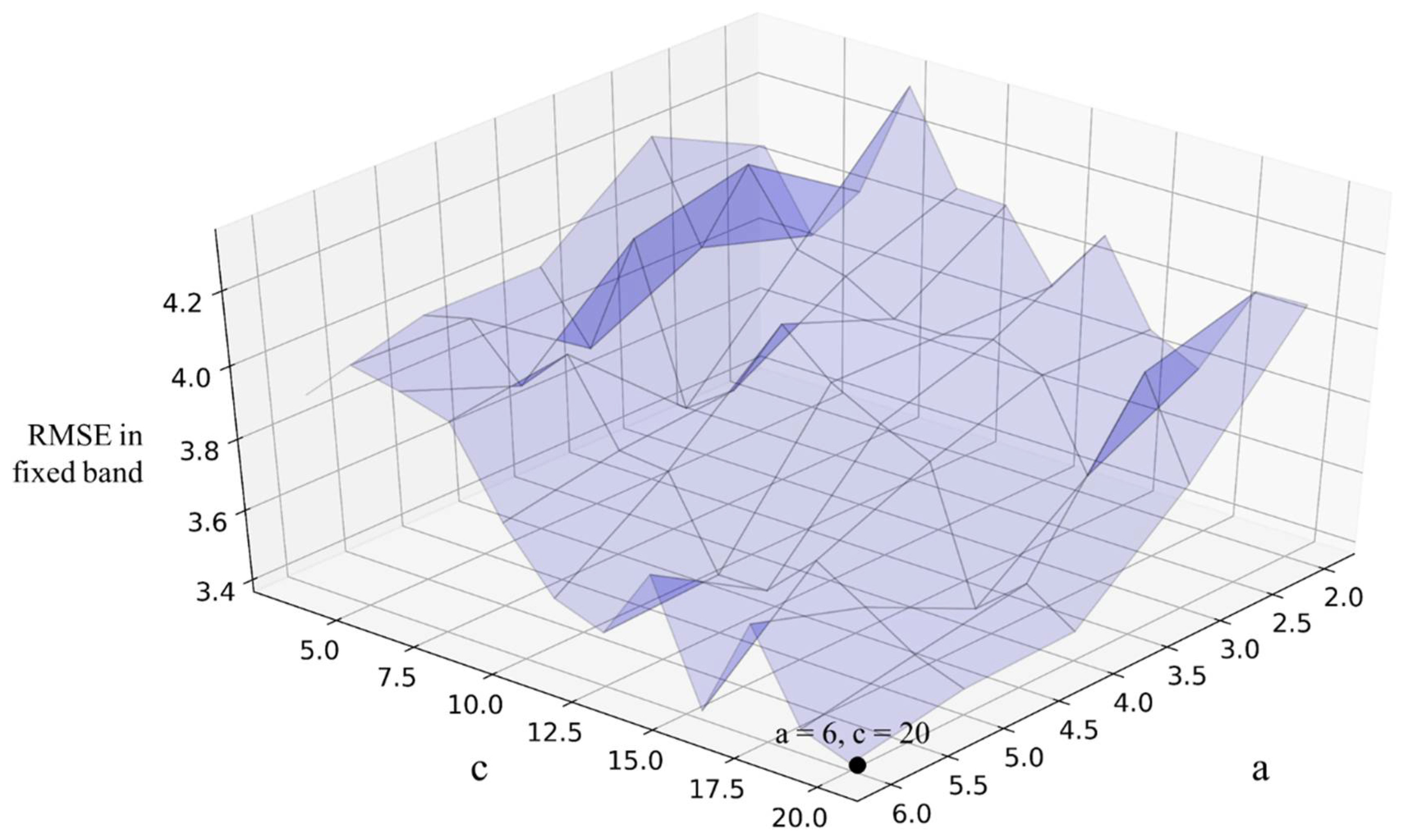
The Gaussian coefficients in Equation (4) controlled the weights at the peak and band width, and the LSTM models with their different combinations were compared with the RMSE in the band. It was obvious that the model’s performance depends on how the dynamic weight is given, because the model responds to errors in observations within the band. The Gaussian coefficient b was set at 20 and a fixed band represented a range of 15 to 25 of PM2.5. Coefficient a was changed from 2 to 6 by increments of 1, and coefficient c was changed from 3.5 to 20 by increments of 1.5.
The effect of band width on calibration performance can be observed in Figure 8. The tendency to incline in the right bottom direction indicates that the weight at peak, which means Gaussian coefficient a, mainly determined the performance in a band. It was confirmed that the RMSE value near the peak decreased as coefficient a increased, except when c was 3.5 and 5. In addition, calibration performance near the peak was improved. That is, the calibration performance near the peak can be improved by a given weight. The change in c had no effect. The best performance near the peak was when a = 6 and c = 20. It can be explained that the Gaussian function decreased more slowly near the peak as c increased. Therefore, observations in a fixed band would have similar weights for calculating loss.
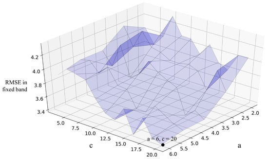
Figure 8.
The change in RMSE in a fixed band with different coefficients for the dynamic weight. Coefficients a and c determine the height of the peak and the width of the band, respectively. The dynamic weight with coefficients at the black point on the graph showed the best calibrating performance in a fixed band with RMSE of 3.77.
The effect of dynamic weight on loss function is shown in Table 5. The use of a dynamically weighted MSE loss function improved the calibration performance meaningfully in terms of RMSE and MAPE. For the overall calibration performance, a Gaussian-weighted MSE with a coefficient (6, 20, 20) showed the best performance, with an RMSE of 3.06 and MAPE of 61.53. An improvement in calibration performance was observed in the band as the band width increased, while the peak weight and band center remained constant. This is thought to result because the weight decreases more slowly near the peak, as previously mentioned.
Table 5.
Comparison of LSTM models with different combinations of coefficients in a Gaussian-weighted MSE loss function. All RMSEs and MAPEs are represented by their average and standard deviation in parenthesis.
5.2. Effect of Different Weight Functions on Calibration Performance
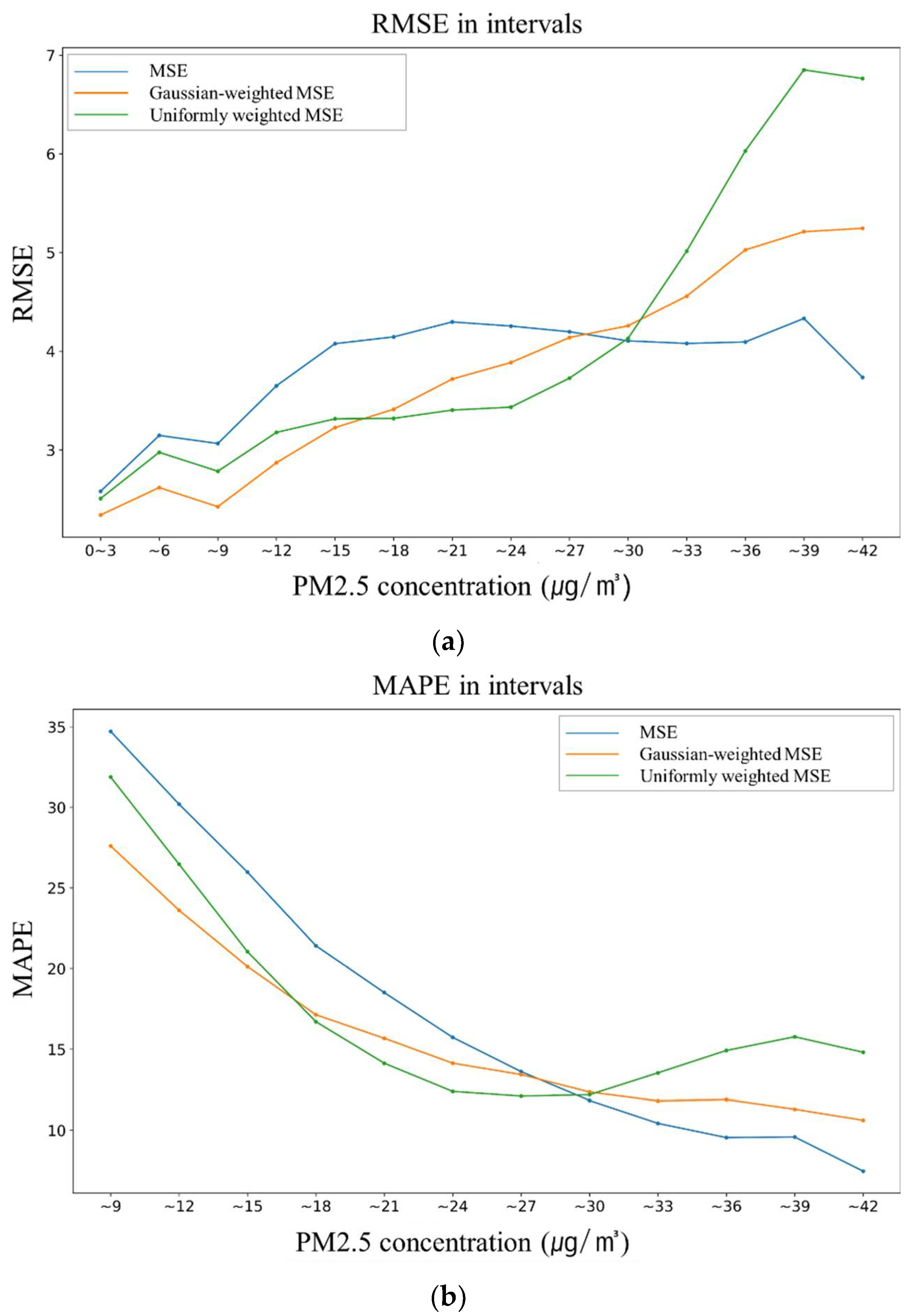
Since coefficients a and c in both bands were similar when the best RMSE was observed, we chose (a, b, c) to be (6, 20, 20). In addition, then, LSTM models with differently weighted loss functions were compared to check the calibration performance within given individual intervals. In the data used as the test set, the interval was divided according to the target value of PM2.5 and the calibration performance. When the target value was very low, the MAPE was highly distorted and meaningless, so it was calculated from a target value of 6 or higher. Both graphs in Figure 9 clearly show that a weighted loss function near the peak improves the calibration performance, causing a trade-off at a concentration of PM2.5 above 30. That is, the RMSE and MAPE values in a given band improved, while they became worse outside of the band. Comparing the MSE with no weight and Gaussian-weighted MSE, under 27 the calibration performance was improved, but it deteriorated above 27. A better improvement and larger trade-off were observed for the uniformly weighted MSE.
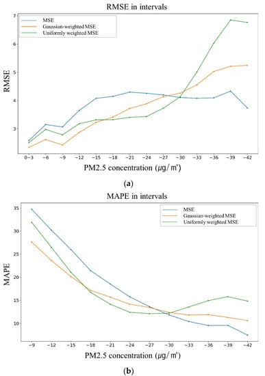
Figure 9.
The calibration performance of the LSTM models with different types of weight functions: (a) the RMSE in each interval; and (b) the MAPE in intervals.
5.3. Effect of the Center of the Weighted Band on Calibration Performance
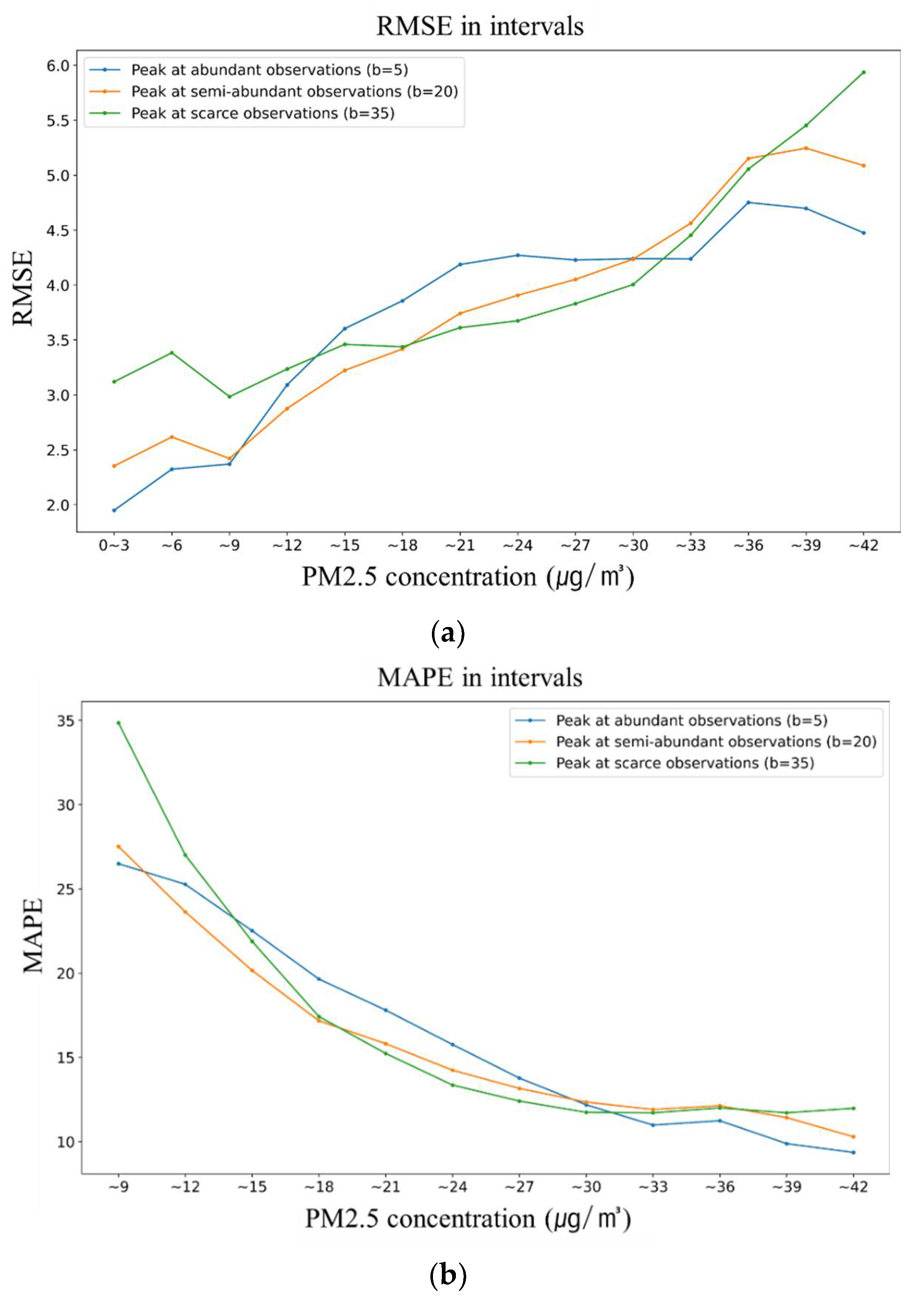
We additionally checked the performance of the model by assigning the band center at 35 μg/m3 of PM2.5, as shown in Table 6. As shown in Figure 10, in the right-skewed data, it was predicted that, when the peak was placed in a section with relatively small observations (b = 35), the performance indicators—RMSE and MAPE—of a very low concentration are lower than those of other cases and, at the same time, they were not improved on the peak. Rather, it performed better by predicting better near the peak, not on the peak. It was even confirmed that the performance slightly improved when the peak was set at 20.
Table 6.
Comparison of the LSTM models with different types and centers of weighted band. All RMSEs and MAPEs are represented by their average and standard deviation in parenthesis.
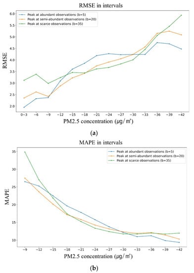
Figure 10.
The calibration performance of the LSTM models with different centers on the weighted band: (a) the RMSE in each interval; and (b) the MAPE in intervals.
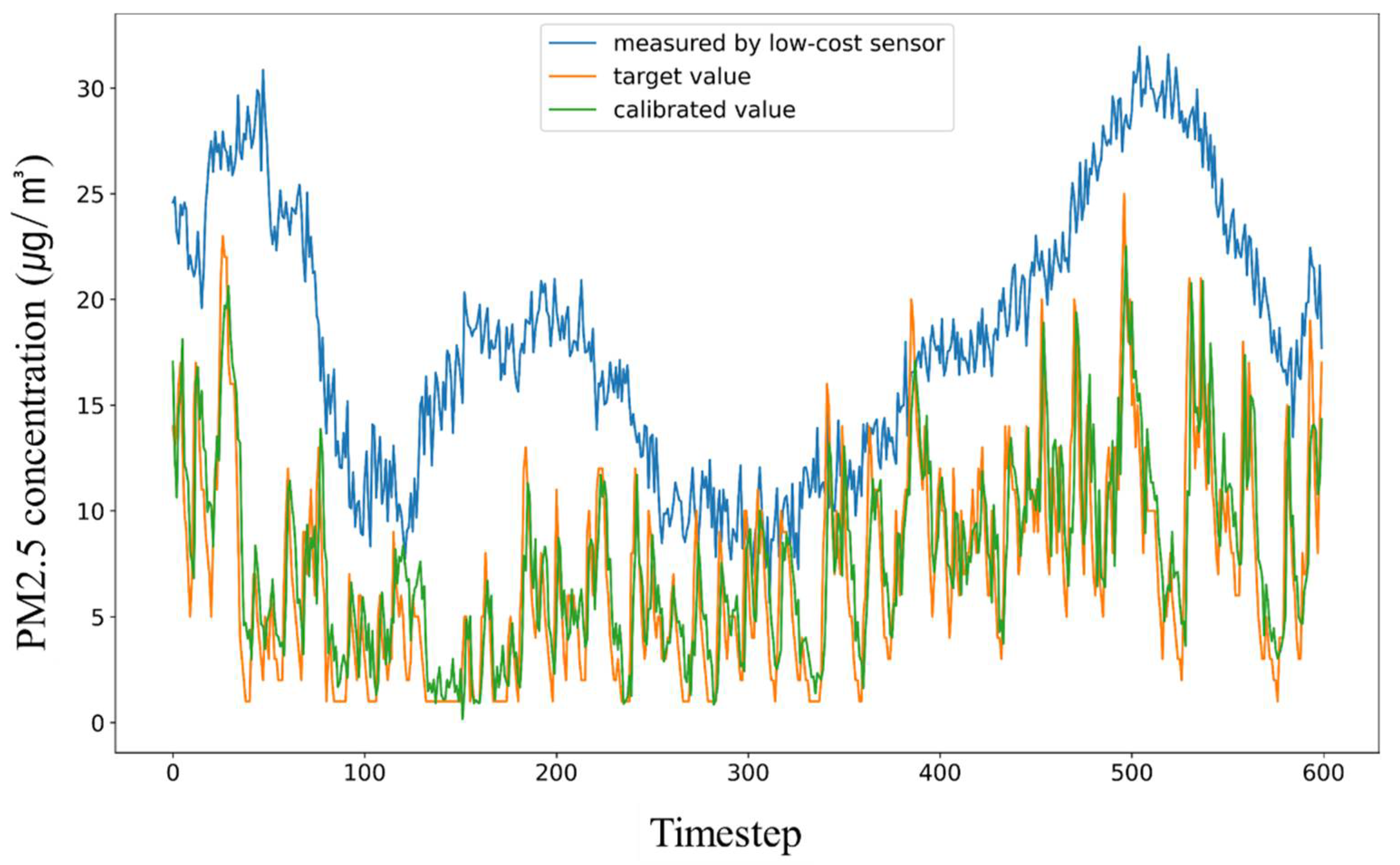
Figure 11 shows the calibration at (6, 20, 20), which exhibited the best calibration performance in Table 5. Its RMSE and MAPE are, respectively, 3.06 and 61.53. The measurement by LCS, shown in blue, was calibrated coercively and resulted in the green plot, which is very similar to the target plot in orange. This result illustrates that the calibration was successful.
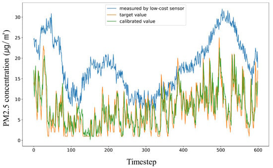
Figure 11.
The result of calibration using the LSTM model with Gaussian-weighted MSE loss function. Only the first 600 observations were plotted for visibility.
6. Conclusions
Particulate matter has become a serious environmental issue, and public attention has resulted in heightened demand for daily information about the concentration of particulate matter. As a result, the economic LCS method has come to be widely used for various purposes. However, there is some concern about its inaccuracy due to distortions resulting from its technological limits, meteorological factors and other local environmental conditions. Previous studies have demonstrated that calibration using machine learning algorithms successfully eliminated the inaccuracy to a certain degree.
The present study applied a dynamic weight to the loss function of the LSTM model to obtain further improvement in the calibration of the LCS data. Since the calibration is a regression task, the MSE was used as the loss function in common. We customized the MSE loss function with two types of weights, Gaussian and uniform weights. The performance of the LSTM model with the loss functions was investigated with different combinations of coefficients. The best calibration performance with dynamically weighted loss function was 3.06 in terms of RMSE, improved by about 12.57% from 3.50, compared to the case without weights. The calibration performance only in the band improved from 4.25 to 3.77.
For our experiment and analysis, an LCS was installed at the research site to collect data under the same conditions as the reference concentration obtained by authorized government measurements. Data about distortion factors from previous studies were collected together. The hyperparameters were optimized by careful trial and error and individual models with different weights were implemented to find the best performance. The performance was evaluated using average RMSE and MAPE from iterations, to avoid random aspects, especially with regard to the initialization of weights and bias in the LSTM model. Further development for the generalization of the suggested calibration methodology can be achieved by setting up more sensors and measuring longer periods in future research.
It was concluded that further improvement in calibration could be achieved by applying dynamic weight to semi-abundant or abundant observations (i.e., big data). It is also suggested to apply dynamic weight on band wide enough to cover the full range of target values. When the Gaussian-shaped weight was applied, the calibration performance of the LSTM model smoothly improved, going to the tail. The uniform weight on a given band resulted in better calibration, but it also resulted in a larger trade-off out of the band. Therefore, the type of weighting function should be considered in relation to the purpose. In terms of the overall performance of the calibration model, the Gaussian weight was more recommendable than uniform weight in this study.
It should be noted that this study was based on a relatively simple task for the LSTM model, because calibrating LCS does not require multistep regression. If a more difficult task is given, and thus the LSTM model becomes more complex, the effect of dynamic weights may appear differently. In addition, it should be noted that the concentrations of particulate matter collected as data were relatively low. The application of our LSTM model to higher concentrations should be further tested in the future. The coefficients for weighting function in this study were optimized for each distribution by calculating the RMSE in a band.
Another notable lesson was that data distribution should be considered in advance, before determining the coefficients of dynamic weights. In this study, observations with PM2.5 concentrations larger than 33 μg/m3 were only 4.5%, 7.4%, and 1% of the training, validation, and test sets, respectively. It is thought that the positive skewness of data in this study resulted in the unsuccessful improvement at the right tail, while improvement was shown in the other parts of the observations.
Author Contributions
Conceptualization, J.R. and H.P.; methodology, J.R. and H.P.; software, J.R.; validation, J.R. and H.P.; formal analysis, J.R.; investigation, J.R.; resources, J.R.; data curation, J.R.; writing—original draft preparation, J.R.; writing—review and editing, H.P.; visualization, J.R.; supervision, H.P.; project administration, H.P.; funding acquisition, H.P. All authors have read and agreed to the published version of the manuscript.
Funding
This research was supported by the Basic Science Research Program through the National Research Foundation of Korea (NRF) funded by the Ministry of Education grant number [2018R1D1A1B07050208] and by Disaster-Safety Platform Technology Development Program of the National Research Foundation of Korea (NRF) funded by the Ministry of Science and ICT grant number [2019M3D7A1094364].
Data Availability Statement
Not applicable.
Conflicts of Interest
The authors declare no conflict of interest. The funders had no role in the design of the study; in the collection, analyses, or interpretation of data; in the writing of the manuscript, or in the decision to publish the results.
References
- WHO. Health Effects of Particulate Matter: Policy Implications for Countries in Eastern Europe, Caucasus and Central Asia; WHO: Geneva, Switzerland, 2013; Volume 1, pp. 2–10.
- WHO. 7 Million Premature Deaths Annually Linked to Air Pollution; WHO: Geneva, Switzerland, 2014. Available online: https://www.who.int/news/item/25-03-2014-7-million-premature-deaths-annually-linked-to-air-pollution (accessed on 30 March 2022).
- Jung, H.J. The Impact of Ambient Fine Particulate Matter on Consumer Expenditures. Sustainability 2020, 12, 1855. [Google Scholar] [CrossRef] [Green Version]
- Cho, E.M.; Jeon, H.J.; Yoon, D.K.; Park, S.H.; Hong, H.J.; Choi, K.Y.; Cho, H.W.; Cheon, H.C.; Lee, C.M. Reliability of Low-Cost, Sensor-Based Fine Dust Measurement Devices for Monitoring Atmospheric Particulate Matter Concentrations. Int. J. Environ. Res. Public Health 2019, 16, 1430. [Google Scholar] [CrossRef] [PubMed] [Green Version]
- Choi, S.; An, J.; Jo, Y. Review of analysis principle of fine dust. Korean Ind. Chem. News 2018, 21, 16–23. [Google Scholar]
- Gao, M.L.; Cao, J.J.; Seto, E. A distributed network of low-cost continuous reading sensors to measure spatiotemporal variations of PM2.5 in Xi’an, China. Environ. Pollut. 2015, 199, 56–65. [Google Scholar] [CrossRef] [Green Version]
- Bodor, M. A Study on Indoor Particulate Matter Variation in Time Based on Count and Sizes and in Relation to Meteorological Conditions. Sustainability 2021, 13, 8263. [Google Scholar] [CrossRef]
- Liang, C.J.; Yu, P.R. Assessment and Improvement of Two Low-Cost Particulate Matter Sensor Systems by Using Spatial Interpolation Data from Air Quality Monitoring Stations. Atmosphere 2021, 12, 300. [Google Scholar] [CrossRef]
- Holder, A.L.; Mebust, A.K.; Maghran, L.A.; McGown, M.R.; Stewart, K.E.; Vallano, D.M.; Elleman, R.A.; Baker, K.R. Field Evaluation of Low-Cost Particulate Matter Sensors for Measuring Wildfire Smoke. Sensors 2020, 20, 4796. [Google Scholar] [CrossRef]
- Matos, T.; Faria, C.L.; Martins, M.S.; Henriques, R.; Gomes, P.A.; Goncalves, L.M. Development of a Cost-Effective Optical Sensor for Continuous Monitoring of Turbidity and Suspended Particulate Matter in Marine Environment. Sensors 2019, 19, 4439. [Google Scholar] [CrossRef] [Green Version]
- Trilles, S.; Vicente, A.B.; Juan, P.; Ramos, F.; Meseguer, S.; Serra, L. Reliability Validation of a Low-Cost Particulate Matter IoT Sensor in Indoor and Outdoor Environments Using a Reference Sampler. Sustainability 2019, 11, 7220. [Google Scholar] [CrossRef] [Green Version]
- Jagatha, J.V.; Klausnitzer, A.; Chacon-Mateos, M.; Laquai, B.; Nieuwkoop, E.; van der Mark, P.; Vogt, U.; Schneider, C. Calibration Method for Particulate Matter Low-Cost Sensors Used in Ambient Air Quality Monitoring and Research. Sensors 2021, 21, 3960. [Google Scholar] [CrossRef]
- Sayahi, T.; Kaufman, D.; Becnel, T.; Kaur, K.; Butterfield, A.E.; Collingwood, S.; Zhang, Y.; Gaillardon, P.E.; Kelly, K.E. Development of a calibration chamber to evaluate the performance of low-cost particulate matter sensors. Environ. Pollut. 2019, 255, 113131. [Google Scholar] [CrossRef] [PubMed]
- Jayaratne, R.; Liu, X.T.; Thai, P.; Dunbabin, M.; Morawska, L. The influence of humidity on the performance of a low-cost air particle mass sensor and the effect of atmospheric fog. Atmos. Meas. Tech. 2018, 11, 4883–4890. [Google Scholar] [CrossRef] [Green Version]
- Wanjura, J.D.; Shaw, B.W.; Parnell, C.B.; Lacey, R.E.; Capareda, S.C. Comparison of continuous monitor (TEOM) and gravimetric sampler particulate matter concentrations. Trans. Asabe 2008, 51, 251–257. [Google Scholar] [CrossRef]
- Mei, H.; Han, P.F.; Wang, Y.N.; Zeng, N.; Liu, D.; Cai, Q.X.; Deng, Z.Z.; Wang, Y.H.; Pan, Y.P.; Tang, X. Field Evaluation of Low-Cost Particulate Matter Sensors in Beijing. Sensors 2020, 20, 4381. [Google Scholar] [CrossRef]
- Brattich, E.; Bracci, A.; Zappi, A.; Morozzi, P.; Di Sabatino, S.; Porcu, F.; Di Nicola, F.; Tositti, L. How to Get the Best from Low-Cost Particulate Matter Sensors: Guidelines and Practical Recommendations. Sensors 2020, 20, 3073. [Google Scholar] [CrossRef]
- Schwarz, A.D.; Meyer, J.; Dittler, A. Opportunities for Low-Cost Particulate Matter Sensors in Filter Emission Measurements. Chem. Eng. Technol. 2018, 41, 1826–1832. [Google Scholar] [CrossRef] [Green Version]
- Zusman, M.; Schumacher, C.S.; Gassett, A.J.; Spalt, E.W.; Austin, E.; Larson, T.V.; Carvlin, G.; Seto, E.; Kaufman, J.D.; Sheppard, L. Calibration of low-cost particulate matter sensors: Model development for a multi-city epidemiological study. Environ. Int. 2020, 134, 105329. [Google Scholar] [CrossRef]
- Badura, M.; Batog, P.; Drzeniecka-Osiadacz, A.; Modzel, P. Evaluation of Low-Cost Sensors for Ambient PM2.5 Monitoring. J. Sens. 2018, 2018, 5096540. [Google Scholar] [CrossRef] [Green Version]
- Sousan, S.; Gray, A.; Zuidema, C.; Stebounova, L.; Thomas, G.; Koehler, K.; Peters, T. Sensor Selection to Improve Estimates of Particulate Matter Concentration from a Low-Cost Network. Sensors 2018, 18, 3008. [Google Scholar] [CrossRef] [Green Version]
- Liu, X.T.; Zhao, Q.; Zhu, S.C.; Peng, W.J.; Yu, L. An experimental application of laser-scattering sensor to estimate the traffic-induced PM2.5 in Beijing. Environ. Monit. Assess. 2020, 192, 1–15. [Google Scholar] [CrossRef]
- Zheng, T.S.; Bergin, M.H.; Johnson, K.K.; Tripathi, S.N.; Shirodkar, S.; Landis, M.S.; Sutaria, R.; Carlson, D.E. Field evaluation of low-cost particulate matter sensors in high-and low-concentration environments. Atmos. Meas. Tech. 2018, 11, 4823–4846. [Google Scholar] [CrossRef] [Green Version]
- Liang, L. Calibrating low-cost sensors for ambient air monitoring: Techniques, trends, and challenges. Environ. Res. 2021, 197, 111163. [Google Scholar] [CrossRef] [PubMed]
- Wang, Y.W.; Du, Y.J.; Wang, J.N.; Li, T.T. Calibration of a low-cost PM2.5 monitor using a random forest model. Environ. Int. 2019, 133, 105161. [Google Scholar] [CrossRef] [PubMed]
- Johnson, N.E.; Bonczak, B.; Kontokosta, C.E. Using a gradient boosting model to improve the performance of low-cost aerosol monitors in a dense, heterogeneous urban environment. Atmos. Environ. 2018, 184, 9–16. [Google Scholar] [CrossRef] [Green Version]
- Loh, B.G.; Choi, G.H. Calibration of Portable Particulate Matter-Monitoring Device using Web Query and Machine Learning. Saf. Health Work. 2019, 10, 452–460. [Google Scholar] [CrossRef]
- Wang, W.C.V.; Lung, S.C.C.; Liu, C.H. Application of Machine Learning for the in-Field Correction of a PM2.5 Low-Cost Sensor Network. Sensors 2020, 20, 5002. [Google Scholar] [CrossRef]
- Li, T.Y.; Hua, M.; Wu, X. A Hybrid CNN-LSTM Model for Forecasting Particulate Matter (PM2.5). IEEE Access 2020, 8, 26933–26940. [Google Scholar] [CrossRef]
- Rengasamy, D.; Jafari, M.; Rothwell, B.; Chen, X.; Figueredo, G.P. Deep Learning with Dynamically Weighted Loss Function for Sensor-Based Prognostics and Health Management. Sensors 2020, 20, 723. [Google Scholar] [CrossRef] [Green Version]
- Ryu, Y.H.; Min, S.K. What matters in public perception and awareness of air quality? Quantitative assessment using internet search volume data. Environ. Res. Lett. 2020, 15, 0940b4. [Google Scholar] [CrossRef]
- Byun, S.; Kim, S.Y. Has Air Pollution Concentration Increased over the Past 17 Years in Seoul, South Korea?: The Gap between Public Perception and Measurement Data. J. Korean Soc. Atmos. Environ. 2020, 36, 240–248. [Google Scholar] [CrossRef]
- Kim, H.; Kang, K.; Kim, T. Measurement of Particulate Matter (PM2.5) and Health Risk Assessment of Cooking-Generated Particles in the Kitchen and Living Rooms of Apartment Houses. Sustainability 2018, 10, 843. [Google Scholar] [CrossRef] [Green Version]
- Hochreiter, S.; Schmidhuber, J. Long short-term memory. Neural Comput. 1997, 9, 1735–1780. [Google Scholar] [CrossRef] [PubMed]
- Yong, Z. Digital Universal Particle Concentration Sensor: PMS7003M Series Data Manual. 2017. Available online: https://eleparts.co.kr/data/goods_old/data/DS_PMS7003M.pdf (accessed on 30 March 2022).
- Model 5014i Beta Continuous Particulate Monitor: Automated Ambient Particulate Measurement Utilizing Beta Attenuation. 2020. Available online: https://www.thermofisher.com/document-connect/document-connect.html?url=https://assets.thermofisher.com/TFS-Assets%2FCAD%2FSpecification-Sheets%2FD00882.pdf (accessed on 30 March 2022).

Publisher’s Note: MDPI stays neutral with regard to jurisdictional claims in published maps and institutional affiliations. |
© 2022 by the authors. Licensee MDPI, Basel, Switzerland. This article is an open access article distributed under the terms and conditions of the Creative Commons Attribution (CC BY) license (https://creativecommons.org/licenses/by/4.0/).