Abstract
Japan is becoming depopulated, with declining fertility rates and massive urban agglomeration due to emigrations from rural areas, which results in rural–urban disparities. As demographic and social divisions between rural and urban areas increase, maintenance of infrastructure and social facilities becomes much more difficult. For social and demographic sustainability, accurate predictions of long-term population distributions are needed. This study improves the Cohort Component Analysis (CCA) into two aspects of “dependent structure” in the model system. The migration sub-model is expanded to include related structures between available job opportunities and the available workforce in each region, which are specified using the spatial autoregressive model. The advantage of the improved CCA to provides rational future projections by considering the longitudinal changes in the spatial distribution of the workforce. The simulation of the proposed model gives an alternative long-term impact of population distribution in Japan, which is compared with the conventional CCA. The results show that the future Japanese populations will become more concentrated in urban areas, with a lower fertility rate. Furthermore, the manufacturing employees will be attracted to metropolitan areas or to regions with industrial zones, and that the number of retailers will undergo changes over time, even in urbanized areas.
1. Introduction
In developed countries, depopulation has become a global phenomenon over the last few decades. The primary cause of current depopulation is declining total fertility rates, which result from a process known as demographic transition [1]. Fertility rates for women of all age groups have declined since 1950, not only in developed countries, but also in developing countries [2]. As the population problem becomes a major concern, an accurate prediction of population development trend has become a top priority, allowing for effective regional planning and decision making [3]. To build effective public plans in regions of depopulation with declining fertility, the structure of population, with its transitions, i.e., the long-term population predictions for the target areas, should be appropriately made.
Cohort component analysis (CCA) is widely used as a standard model for regional population prediction in many developed countries [4,5,6,7], due to its capability for producing key demographic characteristics, including age, gender, natural increase/decease, and social increase/decrease. CCA relies on a simple extension of past trends to provide predictions, and it tends to target the larger levels of geography. In regional planning, population prediction for relatively small areas, such as municipalities, provides fundamental but essential information. Such estimates not only provide population projections for each municipality for long time horizon, but also the spatial pattern of population distribution for some cross-sections, which enables elaborate planning to integrate several public domains [8]. Therefore, with growing demand for detailed demographic information on smaller-scale levels, it is essential to develop the population prediction method, based not only on the assumptions of past trends, but also on the detailed socioeconomic characteristics of each region.
As declining fertility has become a global issue, population prediction, which focuses on fertility rate simulation, has attracted the interest of researchers. Pifarré i Arolas [9] studied the relationship between unemployment and fertility, finding that the higher level of structural unemployment decreases fertility. Policies for increasing fertility rate will not have short-term effects, but they would have significant long-term effects on the population or on economic growth [10]. In population economics, fertility rate (i.e., CWR) is considered to be an aggregated decisions made by females or couples to maximize their utility [11]. In developed countries, women emphasize professional careers and begin postponing family formation and childbearing [12]. Furthermore, the social and economic environments of families with children are substantially different between urban and rural areas. Therefore, the promotion of children in a family requires several policies with complex and comprehensive viewpoints, and countermeasures that account for regional differences in the living environment.
Many recent population studies have focused on migration [13] because it is considered to be the primary demographic transition that shapes national patterns of human settlement [14]. In societies with low fertility and mortality rates, migration has become an important social phenomenon—ones that is relatively more significant in population prediction than birth and death rates. However, most of the previous studies refer to those rates as being a social issue, and so, the quantitative discussion focuses on its impact on spatial settlement patterns. Migration is a phenomenon that is affected by the socioeconomic characteristics of its origin and destination [15] and it can be divided into a couple of spatial domains: international and domestic/internal, but the interests of them are not symmetrical. In contrast, only a few quantitative population prediction studies have focused on domestic/internal migration. Previous studies [16,17] have shown interest towards international migration, due to the economic or social conflict between migrants and residents, while less attention is paid towards internal migration, even though the volume of internal migrants is greater than the international migrants. Migration is more responsive to short term policies, whereas fertility rate is a parameter regarding long-term decision making, and it is not well known whether it is responsive or stable in response to changes in policy options [10]. Therefore, internal migration prediction needs to be justified with spatially heterogeneous parameters, and with the use of complex prediction methods, especially on the subnational level [18]. To improve the effectiveness of spatial population prediction models, much more attention should be paid to internal migration.
Domestic migration is also essential for the study of agglomeration economies. Economic motivations such as land use policies and house price dynamics [19], and income and job opportunities [20], are factors into domestic migration. Additionally, environmental factors such as climate change, rapid-onset events (e.g., hurricanes or tsunamis) and seismic activity also influence the determinants of migration flows [21]. The impacts vary depending on the stage of national development, but rapid domestic migration can lead to an imbalance between the supply and demand of infrastructure in both urban and rural regions. Therefore, domestic migration and economic growth need to be much more focused. The Japan Policy Council argued that the migration of young cohorts from rural regions to urban regions has indirectly caused the nation’s average fertility to decrease. Rural-to-urban migration and the interaction of agglomeration economies in urban areas can generate a negative relationship between income and fertility across regions [22]. This finding is supported by Liao et al. [23], who found that work-seeking domestic migration and fertility decisions interplay within the process of economic development, and that migration and fertility rates are higher in less-developed areas than in areas with advanced economies. Domestic migration also promotes regional innovation [24]. Matanle [25] pointed out that the industrialization and urbanization that occurred in Japan throughout the post-World War II era was accompanied by rapid economic growth. Domestic migration has long-term impacts on regional economic prosperity; it acts as a regulating valve, assisting with achieving the efficient allocation of economic resources across regions. In China, more than 100 million seasonal workers migrated internally in 2004 [26], and according to a 2001 census, India had more than 300 million migrants flow into urbanized areas [27]. These studies highlight the deep interaction between domestic migration and working opportunities or industrial structures.
Our study contributes to the literature by proposing a novel method for modeling future demographic structures. This proposed method combines CCA with a migration model that includes spatial dependencies. Specifically, this study applies spatial dependencies to predict the migration of specific cohorts at the municipality level, using the SAR model. We then combine the predicted migration outputs with the natural change population, calculated through CCA, to obtain the predicted cohort-based population for a first interval year. This population calculation can then be repeated until a final target year is reached. A comparison of repeated applications for the proposed model with the existing CCA method is performed, to clarify impacts upon the projected future population. With this development, the following three questions are set to be answered. The first question is how heterogeneous CWR will affect on the transitions in the population distribution of children, women, and the elderly in municipalities, compared with conventional CCA. The second question is which cohort will be more attracted to urban agglomeration in the output of the proposed CCA model. The third question is how interregional migration in our model is related to the level of urbanization. This question will be tested through the use of urbanized indices in terms of the industrial characteristics.
The remainder of this paper is organized as follows. In Section 2, we present previous studies on population predictions and spatial dependencies. Section 3 reviews the literature on the Japanese population, as well as its urbanization and migration trends. In Section 4, we explain the existing CCA methodology used for national population prediction. In Section 5, we develop our proposed methodology that integrates CCA with the SAR model to analyze population distribution, predict future demographic structures, and summarize the estimated results. In Section 6, we present a comparison of existing CCA predictions with the results of our proposed approach. We also discuss population distribution in terms of urbanization indices and population translation in terms of CWR. Concluding remarks and future challenges are presented in Section 7.
2. Review of the Literature
A review of previous studies revealed that population predictions are calculations of future population development, based on certain assumptions regarding the evolution of the components of demographic change, which are typically made based on the latest trends [18]. This trend-oriented model implicitly includes many socioeconomic factors. Since Malthus proposed the well-known mathematical model for growth estimation under unlimited resources in 1798, many models have been developed with more tractable structures to meet regional planning requirements. Although time-series regression models provide adequate population prediction power [28], they do not reflect the dynamics of demographic subgroups. A cohort is a special population group, often defined by sex and age, in population prediction. Cohort studies were originally developed in medical, demographic, and generational studies because they allow for the examination of specific groups of interest, such as place of residence, occupation, or environmental exposure [29]. Cohort component analysis (CCA) examines cohorts and certain parameters, such as mortality rate, fertility rate or child–woman ratio (CWR), and migration rate [15,30]. CCA has the advantages of simplicity and interpretability, and it is used as a standard model for regional population prediction in the U.S., Japan, and other countries [4,5,6,7]. For instance, Vanella and Deschermeier [31] proposed a probabilistic CCA that uses simulation techniques based on stochastic models for fertility, mortality, and migration, to forecast the population according to age and sex. In addition, Smith et al. [6] conducted a population prediction under acceptable parameter assumptions using different sources of data.
Several population studies have focused on the domestic migration rate, but only a few have focused on the spatial dependence between neighboring regions [32]. When spatial dependence is substantial, its inclusion in modeling will improve the quality of the population prediction [33]. The reason for these dependencies is that the spatial extent of daily activities is often not closed in a municipality to live. As demography is an inherently spatial social science, especially for small areas [34,35], its demographic trends are not specifically observed at an area, but also at the neighboring areas of the area [36]. In other words, the functions of daily activities, such as work, shopping and healthcare are actually supported among the neighborhoods of that municipality. Economic or social factors, such as the labor force requirements of local industries, wholesalers, and retailers, might affect the number of migrations, as well as the spatial dependency. However, it is also possible that there is a reverse causal relationship, in which the locations of the above factors are influenced by the populations of the neighboring regions. Thus, the causal relationships between economic or social factors and migration or population is bidirectional. A model that includes spatial dependency can clarify whether specific cohorts are attracted to urban areas, thereby causing spatial agglomeration.
Developing a population prediction method that incorporates spatial dependency regarding migration and changes in industrial distribution into a CCA would, due to its recursive structure, yield a probable future development path of population and industry. Spatial models describe spatial dependencies among neighbors, and recent developments in statistics and computing resources have allowed for the explicit modeling of spatial relationships [37]. Among these spatial statistical models, the spatial autoregressive (SAR) model is the most appropriate for including spatial dependencies [38]. The existing knowledge-based regression approach for population forecasts typically estimates the relationships between population changes and its causal factors in the estimation period, and then applies the estimated parameters for population projection. The regression approach for population forecasting is being increasingly used in urban planning, climate change and infrastructure systems, because the regression approach does not only provide population projections, but also estimate the relationships between population change and its possible driving factors. [39].
Previous studies regarding with Japanese demography [25] are mainly focused on larger geographic scales—at the national or prefecture levels. However, in recent years, interest in the migration phenomenon has been changed for much smaller spatial units, so as to consider the spatial heterogeneity. Smaller spatial units of demographic studies have been conducted; for example, Stawarz et al.’s internal migration study of Germany (which played a vital role in the creation of Japan’s current local government) [19], or the prediction of the Southern California population by Feng et al. [40]. Our study’s approach was made at the municipality level, such as “shi” (city) and “chō-son” (town and village). According to our knowledge regarding literature reviews, this study is the first comprehensive attempt to apply the SAR model for the labor force movement among the municipalities in Japan as a sub model of population prediction.
3. Description of the Japanese Population, Migration, and Urbanization Trends
In Japan, emigration from rural regions to larger cities has continued since the 1950s, and the total population of the country has decreased since 2009, because of a declining number of births. According to Figure 1a, the annual number of births in Japan has declined from 1.9 million in the 1970s, called the “secondary baby boom,” to 1.01 million in 2015, and the number of deaths has continuously increased from 1980 to 2015. In Japan, the total fertility decreased to below 2.0 in 1975, and it bottomed out at 1.26 in 2005, which was the lowest observation since World War II. In 2015, the rate increased to 1.46; however, this was still far below the replacement level of fertility. Among the Japanese prefectures in 2015, Okinawa had the highest fertility rate of 1.94, while Tokyo had the lowest fertility rate of 1.17.
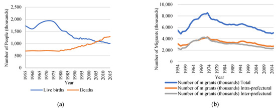
Figure 1.
(a) Live births and deaths in Japan; (b) Number of domestic migrants in Japan.
Japan has also been facing a rapid aging problem over recent decades, and this aging problem will become more intense when the second baby-boomer generation reaches their 60s in 2040. According to the OECD Regional Statistics, while the working-age population in Japan declined by 8.5%, the elderly population increased by 32%, accounting for over a quarter of the Japanese population in 2014. Rural areas in Japan are aging faster than urban ones. Almost 30% of the population in rural areas is over 65 years old, while it is under a quarter of the population in urban areas. In a depopulated society, economically active/working-age groups face particular tension. They must support and educate younger generations while also providing older generations with health care or nursing. Moreover, the country will also face the problem of fewer younger generations being able to join the workforce because of declining birth rates. The causes of the steep drop in births in Japan are as follows: social support for families, in which both parents work outside the home, is scarce, and childcare support from retired generations has become difficult because more households are separated; that is, there are fewer multi-generational households. Because of the pressure to work for economic reasons, many families of reproductive age tend to forgo having children. Even though the above circumstance is not severe in rural areas, which have higher fertility rates, social migration to urban areas, mainly due to job searching, has continued. This will accelerate the population decline, owing to the lower fertility rate in urbanized areas.
As shown in Figure 1b, the number of annual domestic migrants peaked during the mid-1960s and early 1970s. This is due to industrial development during this period, which caused population movements for employment reasons in the industrial sector. After 1972, the number of interregional migrants drastically decreased, due to the severe economic challenges faced by the industrial sector, such as the 1973 oil crisis. Rapid industrialization and urbanization disrupted the balance of the spatial distribution of the population, and urban areas absorbed this inflow by expanding outward into the suburbs. This caused the Tokyo metropolitan area to become one of the largest cities in the world, and exacerbated depopulation in the countryside of Japan. The migration rate increased again after 1995, and the number of inter-prefectural migrants increased yet again after 2011. According to the 2015 population census [41]—eight prefectures, including three metropolitan areas (Tokyo, Osaka, and Nagoya)—had a positive net migration, while the other thirty-nine prefectures had a negative net migration. This statistic shows that Japanese people are highly mobile from rural areas to urban areas. There are several disadvantages in agriculture, such as lower labor inputs because of mechanization, lower wages, and climate change, all of which make stable management difficult. Moreover, reproductive generations are deterred by the poor availability of services in rural areas, including healthcare, education, and transportation. These factors cause people to move from rural areas to urban ones. As rural regions lose population, they face difficulties in maintaining public facilities and social welfare, such as schools and hospitals. This causes the younger population to migrate from rural areas to larger cities in pursuit of better academic and job opportunities. Such population losses have triggered policy concerns regarding the economic and demographic sustainability of rural areas in Japan.
In recent decades, all economies in developed countries have faced slowdowns due to depopulation and aging. An aging and a declining population leads to a decrease in the labor force. This puts further downward pressure on economic growth, due to reduced production caused by the declining labor force, accompanied by an increasing proportion of retired people. Temporary international immigration to compensate for worker shortages is seen as a possible solution that is quicker and more effective in resolving workforce problems in Japan. In 2015, the population of foreign residents in Japan was 1,752,368, which amounted to 1.4% of the total population, which was an increase of 104,331 from 2010 [41]. However, foreign residents are concentrated in urban, suburban, and industrial zones because the Japanese government restricts foreign immigration to only those with specialized and technical skills. The vast majority of these immigrants are also not allowed to bring their family members, and are expected to return to their respective countries after their terms in Japan has ended. Even though accepting foreign residents in this manner can solve the workforce shortage in Japan, it will not raise national fertility. Therefore, immigration under the current policy of the Japanese government could lead to even more rapid agglomeration and urbanization in existing urbanized areas, and deepen the spiral of community aging and depopulation in rural areas [42]. The arguments by Matanle and Sato suggest that the country’s industrial structure and workforce distribution are related, and thus, determining the relationship between demographic change and the industrial structure of the country is necessary for an adequate description of population dynamics.
4. Existing Methodology: Cohort Component Analysis
The ordinary cohort component analysis (CCA) adopted by the Japanese government relies on a simple extension of past trends to provide predictions. In other words, CCA predicts what the population distribution in a target year would be if the current model structure is repeated. CCA assumes the following parameters for each age and sex group: (1) the initial population, (2) the survival rate, (3) the ratio of children to women in the reproductive generation only, (4) the sex ratio of the 0–4 age cohort, and (5) the migration rate. Table 1 displays the parameter settings for CCA by the Japanese government. The core equation of CCA consists of three components in recursive form, denoted as:
where P(i, t) is the initial population of municipality i at initial year t, and NC(i, t) is the natural increase (or decrease if it is negative) in the difference between births and deaths between t and t + k. NM(i, t) is the net migration: the difference in the number of immigrants and emigrants into or from municipality i, between t and t + k. In this study, k is ordinarily set to 5, because of the Census interval of Japan.
Because the population increases that are not caused by immigration only occur in the first cohort (i.e., when a child is born), the survival rate of the cohort can be used instead of the natural increase. The equation, including the survival rate is shown in Equation (2):


Table 1.
Parameter settings using Cohort Component Analysis (CCA).
Table 1.
Parameter settings using Cohort Component Analysis (CCA).
| Parameter | Descriptions |
|---|---|
| Initial Population (Pin (i, x∼x + n)) | (2010) 5-year age cohorts for both sexes in Japan at the municipality level. |
| Survival Rate (S i, x∼x + n) | |
| Cohort Age-specific Child–Women Ratio (CWR i, x∼x + n) | |
| Relative Disparities forCWRi, t (R i) | |
| Child–Women Ratio () or Fertility Rate () | , is adopted from national population projection data. |
| Sex Ratio (SR) for Ages 0–4 |
where is the survival rate of a cohort in the next period, n = 4 for 5-year age groups, and stand for immigration and emigration of municipality i in the period t to t + k, respectively.
To model the natural increase (childbirth) for the first cohort, we assumed a cohort-based child–women ratio (CWR). CWR is measured at the municipal scale, which assumes that the relative disparities of the municipalities are held, by dividing the total CWR of the municipality by the average CWR of the initial year, 2010. This assumption is commonly introduced for the reference (conventional) CWR and our proposed model. The future CWR for municipalities is calculated by multiplying the average CWR of the predicted intervals, which are adopted from the national population prediction data of Japan, 2010–2040, with the medium-fertility assumption that relative disparities in the municipalities are held. The sex ratio at birth (SR) was set as the average value of 105.2 from the actual observations from 2006 to 2010, and was assumed to be constant for both models.
The population of newly born male and female children after 2015 was calculated according to the following equations:
The CCA in this study was based on the initial population in 2010 from the population census of Japan by the Statistics Bureau, Ministry of Internal Affairs and Communications [43], to predict the population in 2015. The predicted population in 2015 was applied again as the initial (input) population in 2020, and the above procedure was repeated until 2040. To predict the population from the base year to the subsequent year, the survival rates according to age and sex are required. The survival rates obtained from the two life tables for subsequent periods are necessary. Life tables are used to measure the mortality, survivorship, and life expectancy of a population of varying ages. In our study, we used the cohort-based life table of the Japanese population in 2010, where age x∼x + 4 is expressed as x years of cohort, and year t = 2010, 2015, 2020, …, 2035.
On the statistics of migration, the population in Japan shows a tendency for exits to exceed entries in terms of international migration. In addition, the net domestic migration by sex was relatively stable. Therefore, the 2012 population projections for Japanese municipalities by the National Institute of Population and Social Security Research Japan assumed the averages of the sex- and age-specific net migration rates between 2004 and 2009 (using the values for four years, and excluding the maximum and minimum values for each age) and smoothed out the rates to remove random fluctuations. These were then set as being constant for the net migration rate of Japanese people for 2015 and onward. In the national population prediction method (CCA), the migration parameter is assumed to be constant, which is not reliable for predicting for the transition trend, and other spatial dependencies, such as workforce cannot be observed.
5. Proposed Model System: Integration of CCA with the SAR Model
The steps of the proposed approach are illustrated in Figure 2. In our approach, the combined models of CCA and spatial statistics were applied for population prediction. The first step of the estimation, which commences from the initial year, is to estimate the surviving population by calculating the age- and sex-specific survival rates for the corresponding cohorts, and to estimate the number of deaths and the child–woman ratio, to obtain the number of births by the end of the interval. This step provides the natural increase and decrease for each cohort at the initial interval. The second step is to apply the natural increase and decrease in each initial cohort, to obtain the population after the interval. The third step is to calculate the immigration and emigration of each cohort during an interval, by applying the SAR model, considering the locations of the industrial workers. These migrant cohorts are social increases or decreases in each municipality, and the predicted population at the end of the interval is obtained. This process is repeated at each interval to reach the final target year.
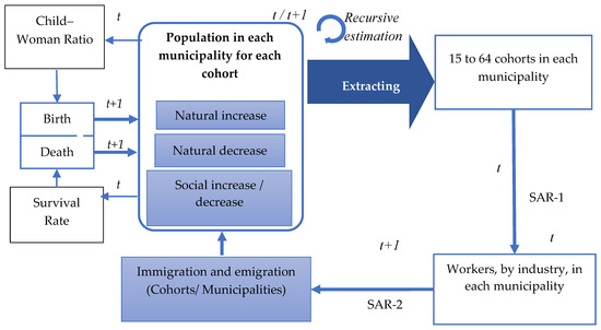
Figure 2.
Proposed prediction methodology flow (integration of CCA with the SAR model).
As shown in Figure 2, the proposed methodology consists of the conventional CCA framework, and of the migration and labor force models, using SAR. These are used to observe the changes in the number of immigrants and emigrants for each cohort, as well as the shifts in retail and manufacturing employees in each interval.
5.1. Spatial Autoregressive Model (SAR)
The following section presents details regarding the SAR model calculations for migration prediction. The spatial dependency among the spatial units was modeled using spatial regression. The models were used to examine the relationship between the dependent variable and the explanatory variables, such as income, employment, and population levels.
The simplest regression model is the standard ordinary least squares (OLS) model, which typically estimates the relationship between a dependent variable and the causal factors. Using OLS to estimate the spatial effects presents a problem: the OLS will not converge to the true values of the parameters. Therefore, a spatial regression model was developed [44]. Understanding the spatial structure assists with the separation of the different potential factors influencing the spatial distribution of the dependent variable. Among the spatial statistical models, the spatial autoregressive (SAR) model is widely applied to calculate the spatial dependency effects on the expected values of the objective variable.
Generally, the concept of the spatial autoregressive model is that neighboring regions have more influence on each other than on distant regions. For example, in region A, a new industry begins operation, which could add several employment opportunities. The inflow of new laborers and their families to region A would increase its population. Some new employees and their families may choose to live in region B, the neighbor of region A, where housing prices are relatively low and well connected with public transport services. In this case, the population growth in region B is caused by the population growth in region A.
Spatial dependencies can be measured by using standard global and local spatial statistics. The global and local measures of spatial autocorrelation are Moran’s I and local Moran’s I statistics. To examine the necessity of the SAR model, the estimation of Moran’s I was used. Moran’s I is a correlation coefficient that measures the spatial autocorrelation between a vector of a georeferenced variable and its spatial lag; that is, the weighted average of the neighboring variables. A higher Moran’s I indicates a stronger spatial autocorrelation or more evident clustering, which should be modeled by a spatial statistical model.
The SAR model is as follows:
The SAR structure can be transferred into an induced form that clearly shows the generating process of the dependent variable, as shown in Equation (6). Anselin [45] noted the model is a “mixed regressive or spatial autoregressive” model.
Vector Y is the georeferenced dependent variable. Matrix X contains exogenous explanatory vectors, and β is the associated regression parameter vector. In our approach, the model will result in a spatial correlation between the explanatory variable and the error term. Therefore, the SAR specification can include the spatial correlation in “Xβ.” SAR was used because we assumed that dependent variable Y (number of migrations) would be an index of regional attractiveness or job opportunities. W is a weighting matrix with neighboring regions, and the associated scalar parameter ρ reflects the strength of spatial dependence. The spatial weight matrix, W, is an nonnegative matrix that has an element of W, which gives the weight at two locations, i and j. In this model, (I − ρW)−1 is non-singular, and product of (I − ρW)−1 , which equals the variance–covariance matrix, is positive-definite. The error vector in Equation (6) shows the dependent structure among the regions. For spatial correlation, we considered the observations as being independent of one another, with each being identically distributed. In this study, we used contiguity matrices to show two spatial correlations with their shared boundary. For contiguity matrices, an element, w[i, j], has a value of 1 if units i and j share a common border, and 0 for the others.
In defining the spatial-weighting matrices, normalization of the matrices is necessary. Generally, there are two types of normalization in the spatial weighting matrices. The first is traditional row normalization:
The second is spectral normalization, which is created by dividing the entries by the absolute value of the largest eigenvalue of the matrix, and is easier to interpret than traditional row normalization.
τ is the largest of the moduli of the eigenvalues of the unnormalized spatial weighting matrix, w*. In this study, we designed the spatial weighting matrices based on spectral normalization.
In spatial statistical models that contain spatial lags of the dependent variables, an interpretation of the parameters is more complicated, as models expand the information set to include information from neighboring regions. This may lead to erroneous conclusions if we use a direct interpretation of the coefficients of the models, such as linear regression models, which can be directly interpreted as the dependent variable, and will affect the explanatory variable. Previous studies [46,47] have suggested that models containing spatial lags of the dependent variable require special interpretation of the parameters. Therefore, in our model, the results were interpreted through a discussion of the direct effect (any given explanatory variable will affect the region itself) and indirect effects (potentially affecting the dependent variable for all other regions). Note that the direct effect is caused by the explanatory variable in the target area, and the indirect effect is caused by the objective variable in neighboring regions, which results in the weighted explanatory variable of the neighboring regions, shown in Equation (6).
In this study, the basic equation, Equation (5), is applied to the industrial employee ( model as SAR model (1), and to the immigration ( and emigration models as SAR model (2).
SAR (1):
SAR (2):
The dependent variable of (SAR-1) is workers by industry, and the explanatory variables are the working-age cohorts (ages 15 to 64). The dependent variables of the migration model (SAR-2) are immigration and emigration by cohort for each municipality. [Migration population, (two types)] × [5-year-old class (19 classes)] × [gender (two types)] = 76 models were estimated. The explanatory variables are the number of retailers and the changes in the number of employees in the secondary industry. In our calculation, the effect of parent migration (20 and above) is also considered in the migration of the child populations (ages 0–4, 5–9, 10–14, and 15–19). In this study, the migration models are estimated separately for immigration, emigration, and industrial characteristics, to clarify the spatially lagged impact of the explanatory variables on the dependent variable. Because of the properties of the regression model, the expected value of the dependent variable, calculated using the estimated model, is consistent with the average of the dependent variable. Therefore, the total number of immigrants and emigrants is consistent with the total of the dependent variable. Therefore, the proposed procedure is consistent with the control total of the data (i.e., the sum of migrants) used in the model estimation. Once the model is estimated, the prediction of the dependent variable is repeated until it reaches the projected year (2040 in our study).
We used the 2010 initial population data from the population census of Japan [48] and estimated data every 5 years from 2015 to 2040. Immigration and emigration, grouped according to cohort and the industrial characteristics, consist of both the Japanese and non-Japanese populations in the municipality. According to the data availability at the municipalities level in 2010, we only incorporated the industrial characteristics as local indices in this study. Usage data were obtained from Geographic Data (ArcGIS Data Collection 2015, Esri Japan) and e-Stat of Japan. The target area included 1858 municipalities. Table 2 presents the descriptive statistics of the variables used in the proposed method.

Table 2.
Descriptive statistics for SAR.
5.2. Summary of SAR Estimation
Our previous study [49] provides a detailed explanation of the model estimation and its results. In this study, we only describe the application of the model steps and summarize the outcome results. Before estimating the population distribution with urbanization factors, we calculated Moran’s I to test the necessity of the spatial statistical model. According to the significance of the Moran’s I test (Table A1), it is appropriate to apply the spatial statistical approach (SAR) in our estimation. The spatial correlation parameters of all working-age cohorts were positive and highly significant in our estimation (Table A2). From these outcomes, we can state that the distribution of the population is indeed affected by urbanization factors (the movement of retailers and manufacturing employees). In our approach, we assumed that the number of retailers represents the geographical characteristics of urban agglomeration, which can explain whether cohorts are attracted to urbanized areas. Regarding the influence of industrial characteristics on the population distribution, we also assumed that primary, secondary, and tertiary employees, and overall industrial employee workforces could be explanatory variables in our model. However, our discussion only focused on the effects of the number of employees from secondary industries (manufacturing industry employees), because they are located in limited areas, such as manufacturing or industrialized zones; for example, the Pacific coastal belt (“Taiheiyo Belt”). The migration of the manufacturing industry’s workforce is the highest among all three industries, which could be a main factor in the expansion of urban areas.
6. Discussion
6.1. Comparison between CCA Output and the Proposed Approach
For comparison, we evaluated our proposed approach (the integration of CCA with the SAR model) against the medium fertility variant population projection for Japan, using conventional CCA (the data for the population projection with conventional CCA are from the Portal Site of the Official Statistics of Japan (E-Stat) [48]). Table 3 displays the differences in the population predictions between the CCA and the proposed approach. Both models showed a decline in the total annual population. In the final predicted year of 2040, the CCA predicted a nationwide population of around 110.92 million, while our approach predicted a decrease in population to around 109.73 million. The children’s cohorts (ages 0–4, 5–9, 10–14, and 15–19) and all of the working-age cohorts (ages 15–64) are predicted to decrease throughout the entire prediction period (2015 to 2040), even though the elderly cohorts (65 and over) will increase in both prediction methods. Our proposed approach predicted fewer children and elderly populations in 2040 than the CCA’s prediction, whereas the predicted population of the working-age cohorts (25–29, 30–34, 35–39, 40–44, 45–49, 50–54, 55–59, and 60–64) in 2040 is higher in our proposed approach than in the CCA.

Table 3.
Population of Japan according to cohort.
The migration prediction results from the CCA with the output of the proposed model (SAR) are shown in Figure 3a,b. The estimated spatial population distribution using the proposed approach was more distinctively different among the municipalities than via the CCA. In the CCA, only urban municipalities will gain immigrants, and most rural municipalities will suffer from emigration. In our approach, rural municipalities also enjoy immigration, as shown in Figure 3b. Our approach observed that population distribution is more skewed, which means that strong population concentrations are present in municipalities that have population attractiveness factors such as industrial development, and that emigration from rural municipalities is larger than immigration, because rural municipalities lack population attractiveness factors. Therefore, we can state that our approach delves deeper into observations of spatial movement or population distribution prediction.
Although future cohort-based populations can be observed in the conventional CCA, potential economic and urbanization indices for future demographic shifts are neglected.
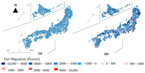

Figure 3.
(a) Net migration for 2040 using CCA; (b) Net migration for 2040 using SAR.
In recent studies, Vollset et al. [50], developed a conventional CCA with statistical models for forecasting mortality, fertility, and migration, to determine the potential economic and geopolitical effects of future demographic shifts. In addition, our previous study [49] clarified the necessity for considering spatial dependencies in population prediction by applying the spatial statistic approach, which can include spatial factors. These studies point out that the integration of CCA with various statistical model analyses, which is highlighted in the present demographic prediction study, is useful for assessing future socioeconomic and urbanization indices. The proposed integration of CCA with a spatial statistical approach enables us to observe the transformation of urbanization factors and the relationship between these factors with population distribution.
6.2. Distribution of Urbanization Indices: Retailers and Manufacturing Employees
Figure 4a,b and Figure 5a,b, respectively, show the distribution of the estimated density of retailers and of manufacturing employees from 2010 to 2040, at the municipality level. From the estimated distribution of retailer densities, in the initial year (2010) in Figure 4a, 130 municipalities had retailer densities that were larger than 1000 persons/km2 (red and orange colors), and these were primarily distributed in four main metropolitan areas (Tokyo, Yokohama, Osaka, and Nagoya). The 1195 municipalities with retailer densities of less than 50 persons/km2 (blue color) were distributed in all of the other areas. However, in 2040, as shown in Figure 4b, only 39 municipalities will have retailer densities that are larger than 1000 persons/km2 (red and orange colors), and the number of municipalities with retailer densities of less than 50 persons/km2 (blue color) will increase to 1300. Comparing the estimated retailer densities during 2010 and during 2040, 73% of municipalities will lose retailer workers by 2040, including the major metropolitan areas.
Among the industrial employee predictions estimated using Equation (10), manufacturing employees is the only variable that can be used to observe the increasing population. In 2010, as shown in Figure 5a, the municipalities with a manufacturing employee density of larger than 1000 persons/km2 (red and orange colors) amounted to 56, most which are distributed within four main metropolitan areas: Tokyo, Yokohama, Osaka, and Nagoya. The number of municipalities with a manufacturing employee density of less than 50 persons/km2 (blue color) was 1100, which were distributed in all other areas. The distribution of manufacturing employees can also be observed in the coastal regions, as specific industrial zones are mainly located on the coast of Japan. As shown in Figure 5b, we can observe that, in 2040, manufacturing employees will be distributed in municipalities with population densities that are larger than 1000 persons/km2 in all 14 major urban areas: Tokyo, Yokohama, Osaka, Nagoya, Sapporo, Fukuoka, Kobe, Kawasaki, Kyoto, Saitama, Hiroshima, Sendai, Chiba, and Kitakyushu. Even in rural areas, 890 municipalities will enjoy an increase in manufacturing employees by 2040.
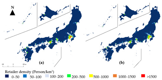
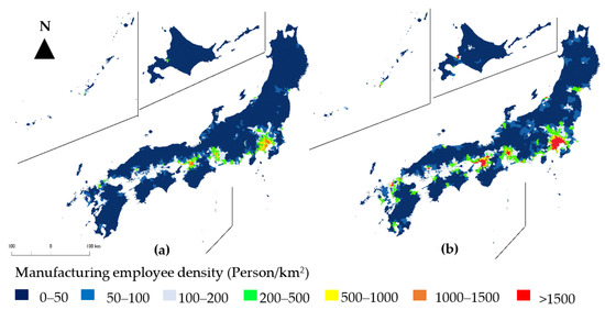

Figure 4.
Distribution of estimated retailer density. (a) Distribution of estimated retailer density in 2010; (b) Distribution of estimated retailer density in 2040.

Figure 5.
Distribution of estimated manufacturing employee density. (a) Distribution of estimated manufacturing employee density in 2010; (b) Distribution of estimated manufacturing employee density in 2040.
We observe that the retailer density will be much more skewed than that of manufacturing employees in 2040. This reveals that in industrial manufacturing, employees will be more attracted to industrialized areas, which might be located in metropolitan or developed regions. The retailer density decreases over time, even in urbanized areas.
6.3. Transition of Population According to Urbanization Indices
In this section, we focus on secondary industry and retail workers as urbanization indicators, and we clarify the correspondence between these indicators and population transitions. We divided the study population into three main population groups: child population (0 to 14 cohorts), female childbearing population (cohorts of women aged 15 to 49), and elderly population (65 and over cohorts). Changes in the urbanization index according to the population of the three groups were observed in a normally distributed bar graph. We confirmed that if the graph tilted to the left, the population moved to urban areas; if it tilted to the right, the population moved to rural areas. By comparing the bell curves of the normal distribution, we can clearly express the differences between 2010 and 2040.
Figure 6a–c indicates the number of retailers compared to the children, female childbearing, and elderly population transitions for 2010 and 2040, respectively. The transitions of all age groups with the number of retailers are normally distributed and skew to the left, which indicates that people will move to urbanized areas with higher retailer indices. From the comparison of the normal distribution curves, we can observe that the number of retailers will decrease by 2040. According to Figure 6d–f, employees in the second industry are normally distributed in all three cohorts, in both 2010 and 2040. The gap in the distributions between 2010 and 2040 clearly shows an increase in the number of employees in secondary industries. Both graphs in 2010 and 2040 are skewed to the left, and the population distribution of employees in the secondary industry moved to the right between 2010 and 2040. Such a transition indicates that a massive population will move from rural areas to urbanized areas. These graphs demonstrate that the future population distribution in Japan will be more concentrated in urbanized areas, whereas rural areas will suffer from depopulation, coupled with a lack of labor.
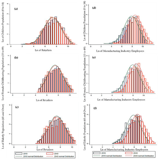
Figure 6.
Distribution of population according to urbanization indices (2010 to 2040). (a) Retailers with children population (0 to 14); (b) Retailers with female childbearing population (15 to 49); (c) Retailers with elderly population (65 and over); (d) Manufacturing industry employees with children population (0 to 14); (e) Manufacturing industry employees with female childbearing population (15 to 49); (f) Manufacturing industry employees with elderly population (65 and over).
6.4. Population Distribution in Terms of Child–Women Ratio (CWR)
To find a factor behind the population distribution over a period, it is essential to examine the spatial distribution of the CWR and the population distribution across all regions, which is significant in terms of the long-term demographic dynamics. Note that we assumed that the relative distribution of the CWR over the region did not change, but that its average over the period changed. According to Figure 7, the average CWR in 2015 was 1.3798. It is expected to gradually decrease until it reaches 1.3302 by 2025, whereupon it will increase slightly starting from 2030, and reach 1.3457 in 2040. The rates have increased slightly as the CWR for women in their 30s and 40s have increased in recent years. Figure 8a,b show the distributions of CWR across all municipalities in 2010 and 2040, respectively, to confirm the relationship between newborn cohorts and the population distribution. From these figures, we can see the spatial distribution of CWR. Some municipalities in Okinawa and Hyogo will enjoy a higher CWR of over 1.9, and 129 municipalities will be consistently above the national average of 1.3457. Almost all urban municipalities, especially Tokyo, Hokkaido, and Kyoto, will have the lowest CWR in 2040.
The relationship between CWR and the three population groups—children, female childbearing, and the elderly—demonstrates how the population is distributed according to the municipalities’ CWRs. Figure 9a–c show the relationship between municipalities’ CWRs and the three groups of populations in 2010 and 2040, respectively. All graphs revealed that the relationship changed over time for all of the age groups. According to Figure 9a, the peak of the CWR with the children’s cohort changes from around 1 in 2010, to around 0.8 2040. The approximated normal curve in 2040 shifted slightly to the left from that in 2010. Figure 9b illustrates that from 2010 to 2040, all female childbearing groups will move from municipalities with higher CWR to those with lower CWR. Figure 9c shows that the spatial distribution of the elderly group was distributed to municipalities with higher CWRs in 2010, and that it will not significantly change by 2040. According to Figure 9a–c, the municipalities with CWRs ranging between 0.8 to 0.9 will have the highest populations for all age groups, and the overall population will shift to municipalities with lower CWRs.
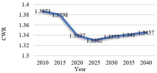
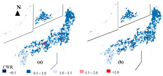
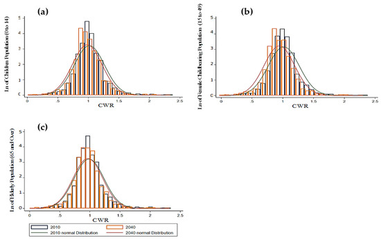

Figure 7.
Medium CWR assumption (Source: https://www.e-stat.go.jp, accessed on 1 March 2021).

Figure 8.
(a) CWRs of municipalities in 2010; (b) CWR of municipalities in 2040.

Figure 9.
Distribution of population by CWR (2010 to 2040). (a) CWR with children population (0 to 14); (b) CWR with female childbearing population (15 to 49); (c) CWR with elderly population (65 and over).
7. Conclusions
Population losses with urban agglomeration in Japan have triggered policy concerns regarding economic and demographic sustainability. To preserve social sustainability, it is essential to understand the agglomeration and depopulation phenomena occurring in Japanese municipalities over the long term. In this study, we proposed an integrated CCA with a spatial statistical approach that can estimate internal migration (immigrants and emigrants) for individual cohorts with spatial dependencies. The estimated results incorporate cohort migration combined with natural increase and decrease prediction, using CCA. Predictions of demographics, population distribution, and the migration of people according to cohort were performed through recursive population estimations.
The conventional CCA only provides information on the future population. However, our approach can provide the distribution of a population and the related urban indices. Our findings prove that the consideration of these factors definitely influences estimations of the future population. This improved population prediction can also assist with clarifying not only the future population’s distribution, but also workforce agglomeration at the municipality level. In this study, we also clarified population movements in terms of CWR to observe shifts in the distribution of children, women, and elderly populations between regions in the future. In addition, by comparing both methods, we can observe how population distributions differ under different assumptions.
The three questions raised with the study’s purpose can be answered as follows. For the first question, the proposed model predicts there will be a slightly smaller total population in 2040 than the conventional CCA. Specifically, the model predicts that there will be fewer children and elderly populations than are predicted when using the CCA. The number of newborns will decrease nationwide; as middle-aged cohorts of childbearing age will be moving to areas with smaller CWR. If this trend continues, Japan’s population will continue to decrease in the future. Regarding the second question, our proposed approach predicts higher populations among the middle-aged cohorts than the conventional CCA. One reason for this outcome is that foreign migrants are counted in our model, because the inclusion of foreign migrants is referenced in the dataset. Foreign migrants will also attract to urbanized areas with more retailers and manufacturing employees. The future population will be highly concentrated in urbanized areas, because domestic migrants will have moved from rural areas to urban areas, and migration from overseas will also be concentrated in urban areas.
Accepting foreign migrants is an effective way to resolve Japan’s workforce needs; however, the national government should design policies that bring benefits to both Japanese people and foreign migrants. Our proposed model observes the influence of the inflow and outflow of foreign migrants on total population predictions, and the findings underscore the need to set up policies to support social services for foreign immigrants in the long term; for example, language support and medical care to compensate for the loss of jobs due to recession, and to manage problems that are related to foreign employees who are permitted to invite family members to stay with them in Japan. Our proposed approach can assist in making meaningful statements for attracting foreign population movements and improving the future of Japan’s demographic distribution, while countering future population aging and declining fertility.
The summary of the answer to the third question is that the number of retailers and manufacturing industry employees affect the population distribution. The estimated results show that the impact of retailers is small, but the impact of manufacturing industry employees is significant. Manufacturing industrial locations are highly skewed toward urbanized areas, and we can conclude that manufacturing industries will be a driving factor in attracting people, especially middle-aged cohorts (15 to 49) from rural areas to urban areas. According to these findings, the nation should make preparations in order to face these challenges, as rapid population movement stimulates the region to make huge investments into their infrastructures. It is essential for Japanese urban areas to find effective and efficient ways to utilize limited resources in order to build a sustainable society. Otherwise, Japanese urban areas could face severe congestion, insufficient infrastructure, health, job, and environmental problems, etc., whereas some areas such as metropolitan Tokyo already struggle to overcome urban agglomeration.
As rapid urban population growth can outstrip the capacity of infrastructure, we should prepare policy implementations based on the 2030 United Nation Agenda, Sustainable Development Goal 11, which is to “make cities and human settlements inclusive, safe, resilient and sustainable”. Based on the estimated long-term population dynamics across all municipalities in Japan, we propose progressive policies for regional sustainable development that could contribute towards finding solutions for the challenges of urban agglomeration and rural depopulation, such as addressing the shortage of daycare facilities to attract female participation in the workforce and the resultant economic growth; introducing advanced transport systems, such as autonomous vehicles, that are more feasible and sustainable than conventional bus or train services; and preserving social services in rural areas via ICT infrastructure to enhance various community services. In addition, the effectiveness of incentives in attracting workers from industrial zones in urban areas to rural communities with innovative technology-based business entities can be demonstrated using the proposed approach.
With our approach, the distribution of migrants and the locations of working opportunities are correlated with the population estimation. In this study, all estimated models showed positive correlations between cohort migration and the urbanization indices. If these relationships change, each cohort prediction will follow. The advantage of the proposed model is in its capacity to consider such relationships in terms of migration and working opportunities. The proposed approach can be used to analyze the significance of local services, natural resources, and local attractiveness, which can be factors for attracting populations to local areas in order to overcome urban agglomeration. Without our modifications, such local attractiveness characteristics cannot be discussed based on conventional CCA. Our approach is one of the options for stabilizing the projection of the future population, and it is substantially allows for observations on the difference between the existing national CCA prediction method, and the results of the proposed approach.
Author Contributions
S.O. and M.T. contributed to the study conception and design. Material preparation, data collection, and analysis were performed by S.O. The first draft of the manuscript was also written by S.O. S.O. and M.T. commented on previous versions of the manuscript. All authors have read and agreed to the published version of the manuscript.
Funding
This research received no external funding.
Institutional Review Board Statement
Not applicable.
Informed Consent Statement
Not applicable.
Data Availability Statement
The data that support the findings of this study are available from the official statistic website-Statistics Bureau of Japan. (https://www.stat.go.jp/english/index.html, accessed on 1 March 2021).
Conflicts of Interest
The authors declare no conflict of interest.
Appendix A

Table A1.
Global Moran’s I Analysis of total migration and industrial variables.
Table A1.
Global Moran’s I Analysis of total migration and industrial variables.
| Variable | Moran’s I | Expected I | Variance | Z-Score | p-Value |
|---|---|---|---|---|---|
| Male Total Immigration | 0.39692 *** | −0.00072 | 0.00856 | 45.28304 | 0.00000 |
| Male Total Emigration | 0.41763 *** | −0.00072 | 0.00859 | 48.67499 | 0.00000 |
| Female Total Immigration | 0.39061 *** | −0.00072 | 0.00857 | 45.66852 | 0.00000 |
| Female Total Emigration | 0.37421 *** | −0.00072 | 0.00556 | 43.8016 | 0.00000 |
| No: of Employees in 2nd Industry | 0.34752 *** | −0.00072 | 0.00726 | 47.94531 | 0.00000 |
| No: of Retailers | 0.34389 *** | −0.00072 | 0.00726 | 47.44475 | 0.00000 |
*** p < 0.001.

Table A2.
Results of spatial correlation parameter for both genders with cohorts.
Table A2.
Results of spatial correlation parameter for both genders with cohorts.
| Cohorts | Spatial Correlation Parameter () | |||
|---|---|---|---|---|
| Male Immigration | Male Emigration | Female Immigration | Female Emigration | |
| 0–4 | 0.196 *** | 0.238 *** | 0.195 *** | 0.056 |
| 5–9 | 0.0868 * | 0.113 * | 0.121 ** | 0.0949 * |
| 10–14 | 0.0848 * | 0.130 ** | 0.152 ** | 0.0895 |
| 15–19 | 0.157 ** | 0.126 * | 0.11 * | 0.0688 |
| 20–24 | 0.137 *** | 0.199 *** | 0.145 *** | 0.0693 |
| 25–29 | 0.142 *** | 0.199 *** | 0.210 *** | 0.185 *** |
| 30–34 | 0.210 *** | 0.294 *** | 0.234 *** | 0.196 *** |
| 35–39 | 0.209 *** | 0.242 *** | 0.234 *** | 0.127 *** |
| 40–44 | 0.117 *** | 0.213 *** | 0.144 *** | 0.0693 * |
| 45–49 | 0.0746 * | 0.135 *** | 0.0987 ** | 0.129 *** |
| 50–54 | 0.0599 | 0.146 *** | 0.181 *** | 0.172 *** |
| 55–59 | 0.0748 | 0.111 ** | 0.212 *** | 0.0979 ** |
| 60–64 | 0.0908 * | 0.0913 * | 0.131 *** | 0.0657 |
| 65–69 | 0.173 *** | 0.198 *** | 0.161 *** | 0.176 *** |
| 70–74 | 0.220 *** | 0.259 *** | 0.292 *** | 0.204 *** |
| 75–79 | 0.284 *** | 0.334 *** | 0.221 *** | 0.101 * |
| 80–84 | 0.349 *** | 0.304 *** | 0.236 *** | 0.0863 |
| 85–89 | 0.284 *** | 0.345 *** | 0.168 *** | 0.0348 |
| 90–over | 0.456 *** | 0.514 *** | 0.193 *** | 0.0934 |
| Total | 0.338 *** | 0.524 *** | 0.415 *** | 0.416 *** |
* ρ < 0.05, ** ρ < 0.01, *** ρ < 0.001.
References
- Lutz, W.; Gailey, N. Depopulation as a Policy Challenge in the Context of Global Demographic Trends. UNDP Serbia. 2020. Available online: http://pure.iiasa.ac.at/16811 (accessed on 1 November 2021).
- Population Reference Bureau. World Population Data Sheet 2021. Available online: https://interactives.prb.org/2021-wpds (accessed on 1 January 2022).
- Chen, L.; Mu, T.; Li, X.; Dong, J. Population Prediction of Chinese Prefecture-Level Cities Based on Multiple Models. Sustainability 2022, 14, 4844. [Google Scholar] [CrossRef]
- Wilson, T.; Rees, P. Recent Developments in Population Projection Methodology. Popul. Space Place 2005, 11, 389. [Google Scholar] [CrossRef]
- Chi, G. Can Knowledge Improve Population Forecasts at Subcounty Levels? Demography 2009, 46, 405–427. [Google Scholar] [CrossRef] [PubMed]
- Smith, S.K.; Jeff, T.; David, A.S. Implementing the Cohort-Component Method. In A Practitioner’s Guide to State and Local Population Projections; The Springer Series on Demographic Methods and Population Analysis; Springer: Dordrecht, The Netherlands, 2013; pp. 155–183. [Google Scholar] [CrossRef]
- Wilson, T. Evaluation of Alternative Cohort-Component Models for Local Area Population Forecasts. Popul. Res. Policy Rev. 2016, 35, 241–261. [Google Scholar] [CrossRef]
- Zoraghein, H.; O’Neill, B.C. US State-level Projections of the Spatial Distribution of Population Consistent with Shared Socioeconomic Pathways. Sustainability 2020, 12, 3374. [Google Scholar] [CrossRef]
- Pifarré i Arolas, H. A Cohort Perspective of the Effect of Unemployment on Fertility. J. Popul. Econ. 2017, 30, 1211–1239. [Google Scholar] [CrossRef]
- Parsons, A.J.Q.; Stuart, G. An evaluation of fertility- and migration-based policy responses to japan’s ageing population. PLoS ONE 2018, 13, e0209285. [Google Scholar] [CrossRef]
- Gary, S.B. An Economic Analysis of Fertility. In Demographic and Economic Change in Developed Countries; Columbia University Press: New York, NY, USA, 1960; pp. 209–240. Available online: http://www.nber.org/chapters/c2387 (accessed on 20 July 2021).
- Caltabiano, M.; Rosina, A. An Analysis of Late Fertility in Italy: The Role of Education; Atti della Riunione Scientifica della Società Italiana di Statistica; Università degli Studi di Padova: Padova, Italy, 2010; pp. 1–8. [Google Scholar]
- Lucas, R.E.B. Internal Migration in Developing Economies: An Overview; KNOMAD Working Paper No. 6; Global Knowledge Partnership on Migration and Development (KNOMAD): Washington, DC, USA, 2015. [Google Scholar]
- Rodríguez, J.; Rowe, F. Internal Migration and Spatial De-Concentration of Population in Latin America. 2018. Available online: https://www.niussp.org/migration-and-foreigners/internal-migration-and-spatial-de-concentration-of-population-in-latin-america/ (accessed on 1 November 2021).
- Lutz, W.; Amran, G.; Bélanger, A.; Conte, A.; Gailey, N.; Ghio, D.; Grapsa, E.; Jensen, K.; Loichinger, E.; Marois, G.; et al. Demographic Scenarios for the EU: Migration, Population and Education; Publications Office of the European Union: Luxembourg, 2019. [Google Scholar]
- Cohen, J.E.; Roig, M.; Reuman, D.C.; GoGwilt, C. International Migration beyond Gravity: A Statistical Model for Use in Population Projections. Proc. Natl. Acad. Sci. USA 2008, 105, 15269–15274. [Google Scholar] [CrossRef]
- Beauchemin, C. A Manifesto for Quantitative Multi-Sited Approaches to International Migration. Int. Migr. Rev. 2014, 48, 921–938. [Google Scholar] [CrossRef]
- Reinhold, M.; Stephan, L.T. Subnational Population Projections by Age: An Evaluation of Combined Forecast Techniques. Popul. Res. Policy Rev. 2015, 34, 593–613. [Google Scholar] [CrossRef]
- Stawarz, N.; Sander, N.; Sulak, H. Internal migration and housing costs—A panel analysis for Germany. Popul. Space Place 2021, 27, e2412. [Google Scholar] [CrossRef]
- Murayama, K.; Nagayasu, J. Toward Coexistence of Immigrants and Local People in Japan: Implications from Spatial Assimilation Theory. Sustainability 2021, 13, 3849. [Google Scholar] [CrossRef]
- Hoffmann, R.; Dimitrova, A.; Muttarak, R.; Cuaresma, J.C.; Peisker, J. A meta-analysis of country-level studies on environmental change and migration. Nat. Clim. Change 2020, 10, 904–912. [Google Scholar] [CrossRef]
- Sato, Y. Economic Geography, Fertility and Migration. J. Urban Econ. 2007, 61, 372–387. [Google Scholar] [CrossRef]
- Liao, P.; Wang, P.; Wang, Y.; Chong, K.Y. Fertility and Internal Migration. Fed. Reserve Bank St. Louis Rev. Fourth Quart. 2020, 102, 429–445. [Google Scholar] [CrossRef]
- Zhao, X.; Li, X. The influence of internal migration on regional innovation in China. Econ. Res.-Ekon. Istraživanja 2021, 34, 498–520. [Google Scholar] [CrossRef]
- Matanle, P. Towards an Asia-Pacific depopulation dividend in the 21st century. Regional growth and shrinkage in Japan and New Zealand. Asia-Pac. J. 2017, 15, 5. [Google Scholar]
- Deshingkar, P.; Grimm, S. Internal Migration and Development: A Global Perspective; Paper Prepared for International Organization for Migration (IOM); International Organization for Migration: Geneva, Switzerland, 2005. [Google Scholar]
- Deshingkar, P. Internal Migration, Poverty and Development in Asia; Briefing Paper; Overseas Development Institute: London, UK, 2006. [Google Scholar]
- Abel, G.J.; Bijak, J.; Forster, J.J.; Raymer, J.; Smith, P.W.F.; Wong, J.S.T. Integrating Uncertainty in Time Series Population Forecasts: An Illustration Using a Simple Projection Model. Demogr. Res. 2013, 29, 1187–1226. [Google Scholar] [CrossRef]
- Doll, R. Cohort Studies: History of the Method, I. Prospective Cohort Studies. Soz. Prav. SPM 2001, 46, 75–86. [Google Scholar] [CrossRef]
- United Nations, Department of Economic and Social Affairs, Population Division. World Population Prospects 2019: Highlights (ST/ESA/SER.A/423); United Nations: New York, NY, USA, 2019. [Google Scholar]
- Vanella, P.; Descheenie, P. A Probabilistic Cohort-Component Model for Population Forecasting—The Case of Germany. J. Popul. Ageing 2020, 13, 513–545. [Google Scholar] [CrossRef]
- Rees, P.; Martin, B.; Marek, K.; Dorota, K.; Philipp, U.; Aude, B.; Elin, C.-E.; John, S. The Impact of Internal Migration on Population Redistribution: An International Comparison: The Impact of Internal Migration. Popul. Space Place 2017, 23, e2036. [Google Scholar] [CrossRef]
- Pascal, M.; Vérène, W.; Magali, C.; Karine, L.; Aymeric, U.; Pascal, B. Heat and Cold Related-Mortality in 18 French Cities. Environ. Int. 2018, 121, 189–198. [Google Scholar] [CrossRef]
- Voss, P.R. Demography as a spatial social science. Popul. Res. Policy Rev. 2007, 26, 457–476. [Google Scholar] [CrossRef]
- Matthews, S.A.; Parker, D.M. Progress in Spatial Demography. Demogr. Res. 2013, 28, 271–312. [Google Scholar] [CrossRef]
- Wilson, T.; Grossman, I.; Alexander, M.; Rees, P.; Temple, J. Methods for Small Area Population Forecasts: State-of-the-Art and Research Needs. Popul. Res. Policy Rev. 2021, 1–34. [Google Scholar] [CrossRef]
- Schaub, M.; Kéry, M. Combining Information in Hierarchical Models Improves Inferences in Population Ecology and Demographic Population Analyses: Hierarchical Models in Population Ecology. Anim. Conserv. 2012, 15, 125–126. [Google Scholar] [CrossRef]
- LeSage, J.; Robert, K.P. Introduction to Spatial Econometrics, 1st ed.; Chapman and Hall/CRC: Boca Raton, FL, USA, 2009. [Google Scholar] [CrossRef]
- Chi, G.; Wang, D. Small-Area Population Forecasting: A Geographically Weighted Regression Approach. In The Frontiers of Applied Demography; Applied Demography Series; Swanson, D.A., Ed.; Springer International Publishing: Cham, Switzerland, 2017; Volume 9, pp. 449–471. [Google Scholar] [CrossRef]
- Feng, Q.; Wang, Z.; Choi, S.; Zeng, Y. Forecast Households at the County Level: An Application of the ProFamy Extended Cohort-Component Method in Six Counties of Southern California, 2010 to 2040. Popul. Res. Policy Rev. 2020, 39, 9531. [Google Scholar] [CrossRef]
- Statistics Bureau, Ministry of Internal Affairs and Communications. Result of the Population Estimates, 2015 Population Census of Japan; Final Report; Statistics Bureau, Ministry of Internal Affairs and Communications: Tokyo, Japan, 2018.
- Matanle, P.; Sato, Y. Coming Soon to a City Near You! Learning to Live ‘Beyond Growth’ in Japan’s Shrinking Regions. Soc. Sci. Jpn. J. 2010, 13, 187–210. [Google Scholar] [CrossRef][Green Version]
- Statistics Bureau, Ministry of Internal Affairs and Communications. Result of the Population Estimates, 2010 Population Census of Japan; Statistics Bureau, Ministry of Internal Affairs and Communications: Tokyo, Japan, 2012; Volume 7-1.
- Chi, G.; Vos, P. Small-area population forecasting: Borrowing strength across space and time. Popul. Space Place 2011, 17, 505–520. [Google Scholar] [CrossRef]
- Anselin, L. Spatial Econometrics: Methods and Models; Kluwer Academic Publishers: Dorddrecht, The Netherlands, 1988. [Google Scholar]
- Kim, C.; Phipps, T.; Anselin, L. Measuring the benefits of air quality improvement: A spatial hedonic approach. J. Environ. Econ. Manag. 2003, 45, 24–39. [Google Scholar] [CrossRef]
- Anselin, L.; Le Gallo, J. Interpolation of Air Quality Measures in Hedonic House Price Models: Spatial Aspects. Spat. Econ. Anal. 2006, 1, 31–52. [Google Scholar] [CrossRef]
- National Institute of Population and Social Security Research in Japan. Population Projections for Japan. Available online: https://www.ipss.go.jp/index-e.asp (accessed on 9 March 2022).
- Oo, S.; Tsukai, M. Internal Migration Prediction for Economic Development in Japan by Considering the Spatial Dependencies. In Proceedings of the Eastern Asia Society for Transportation Studies, Tokyo, Japan, 25 May 2021; Volume 13. [Google Scholar]
- Vollset, S.E.; Goren, E.; Yuan, C.-W.; Cao, J.; Smith, A.E.; Hsiao, T.; Bisignano, C.; Azhar, G.S.; Castro, E.; Chalek, J.; et al. Fertility, mortality, migration, and population scenarios for 195 countries and territories from 2017 to 2100: A forecasting analysis for the Global Burden of Disease Study. Lancet 2020, 396, 1285–1306. [Google Scholar] [CrossRef]
Publisher’s Note: MDPI stays neutral with regard to jurisdictional claims in published maps and institutional affiliations. |
© 2022 by the authors. Licensee MDPI, Basel, Switzerland. This article is an open access article distributed under the terms and conditions of the Creative Commons Attribution (CC BY) license (https://creativecommons.org/licenses/by/4.0/).