
Research on Multi-Center Mixed Fleet Distribution Path Considering Dynamic Energy Consumption Integrated Reverse Logistics

Abstract
:1. Introduction
2. Materials and Methods
2.1. System Dynamics Model
2.2. Problem Analysis
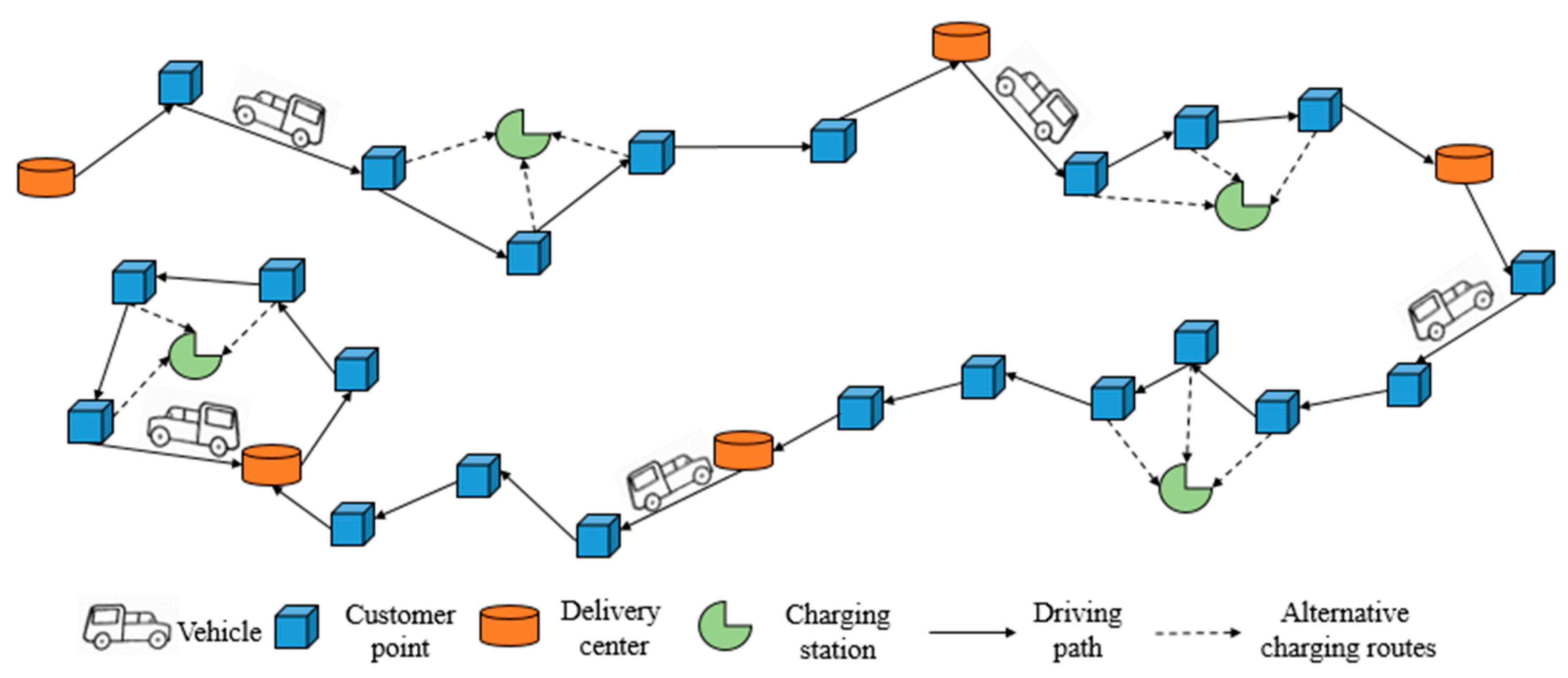
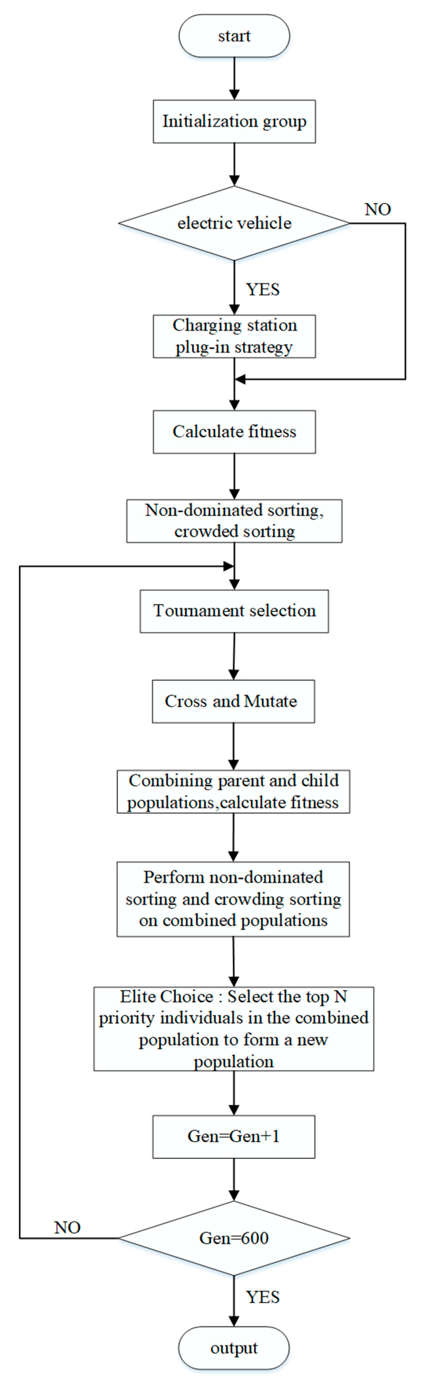
- Select the distribution center from which the vehicle departs and the distribution center where the vehicle returns. The vehicle returns to any distribution center after serving all customers. Two distribution centers (or possibly the same distribution center) are combined with the customer points that satisfy the load of the vehicle to form an initial route;
- Assuming that the vehicle performing the route distribution task is an electric vehicle, it is determined whether the vehicle travel time in the route exceeds the charging and discharging cycle time. If it exceeds, go to step 3, otherwise go to step 4;
- Route is the driving route of the oil truck. If the total weight of the cargo exceeds the maximum load of the vehicle, delete this route; otherwise, store the feasible solution set. If the time to reach the customer point exceeds the time constraint, calculate the penalty cost and opportunity cost;
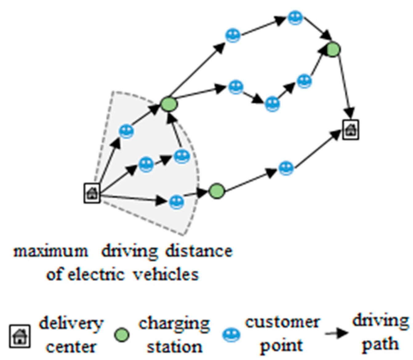
- The route is the driving path of the electric vehicle. If the total weight of the goods exceeds the maximum load of the vehicle, delete this route; otherwise, store the feasible solution set. If the time to reach the customer point exceeds the time constraint, calculate the penalty cost and opportunity cost. If the driving distance does not exceed the maximum driving distance of the electric vehicle, store the feasible solution set; otherwise, add a charging station closest to the customer point that exceeds the maximum driving distance of the electric vehicle and go to step 5;
- If the nearest charging station is added to the customer point that exceeds the maximum driving distance of the electric vehicle and the distance still exceeds the maximum driving distance of the electric vehicle, subtract one customer point and then add the nearest charging station for the new customer Determine whether the distance exceeds the maximum travel distance of the electric vehicle. If it exceeds, go to step 6; otherwise, insert the location index of the charging station between the new customer point and the subtracted customer point, calculate the charging time to reach the charging depth, and go to step 7;
- Subtract one customer point again, add a charging station closest to the new customer, and judge whether the distance exceeds the maximum travel distance of the electric vehicle at this time. If it exceeds, go back to step 5; otherwise, insert the location index of the charging station between the new customer point and the subtracted customer point, calculate the charging time to reach the charging depth, and go to step 7;
- After adding a charging station, determine whether the remaining distance of the path exceeds the maximum travel distance of the electric vehicle. If it exceeds, continue to join the charging station and go to step 4; otherwise, go to step 8;
- Store the feasible solution set.
| Algorithm 1. Pseudo code of charging station plug-in strategy. |
| begin |
| maxenergy = = 50 kWh // maximum energy consumption of electric vehicles |
| = = 10 h // maximum charge–discharge cycle time for electric vehicles |
| calculate drivingtime // calculate vehicle travel time |
| calculate energymatrix // calculate the energy consumption matrix between adjacent nodes of the vehicle |
| calculate minenergy // calculate the energy consumption of driving to the charging station closest to the customer point |
| calculate charge // calculate the number of charges |
| if drivingtime < // determine the type of vehicle, if it is an electric vehicle |
| find((energymatrix (j) + minenergy (j) > ii* maxenergy)&&(energymatrix(j) + minenergy (j) < (ii + 1)* maxenergy)) // find the location of the customer point j that is insufficient for the ii-th charge |
| if energymatrix (j − k) + minenergy (j) < ii* maxenergy // need to be plugged into the charging station after subtracting k customers |
| INDEX = j − k; // calculate index of the location where the charging station needs to be plugged in |
| index = minenergy (j); // calculate the distance to the nearest charging station to j customer point |
| ret = [ret(:,1: INDEX) index ret(:,(INDEX + 1):end)];// form new chromosomes |
| end |
| end |
- For input parameters, input objective function and constraints, select various parameters (population size, crossover rate, mutation rate, etc.,) according to the actual problem;
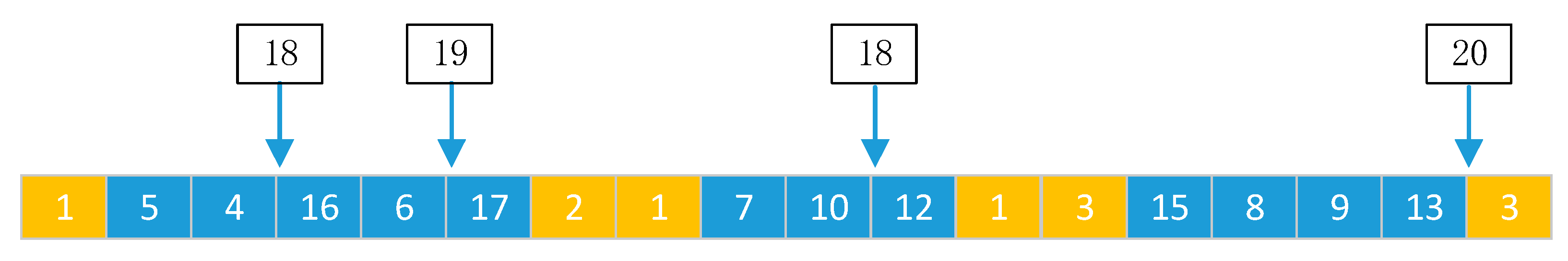
- Initialize the population, encode each node in the logistics distribution network through integer coding, and the individual composed of all nodes represents the vehicle travel path, as shown in Figure 7. When the cargo weight exceeds the vehicle load, return to any distribution center. The chromosome consists of the vehicle departure node, the customer node served by the vehicle, the vehicle return node, and the number of vehicles. For example, the driving route of a vehicle is 3→9→7→6→10→12→1. Randomly generate chromosome combinations to become the initial population.
- The charging station set includes all charging stations, and the same charging station can be repeatedly selected to be inserted into the chromosome; that is, the charging station can be visited multiple times by different routes. According to the charging station plug-in strategy, the routes that need to be inserted into the charging station nodes are re-coded, and the initial population is re-formed, as shown in Figure 8.
- Calculate the fitness of the initialized population;
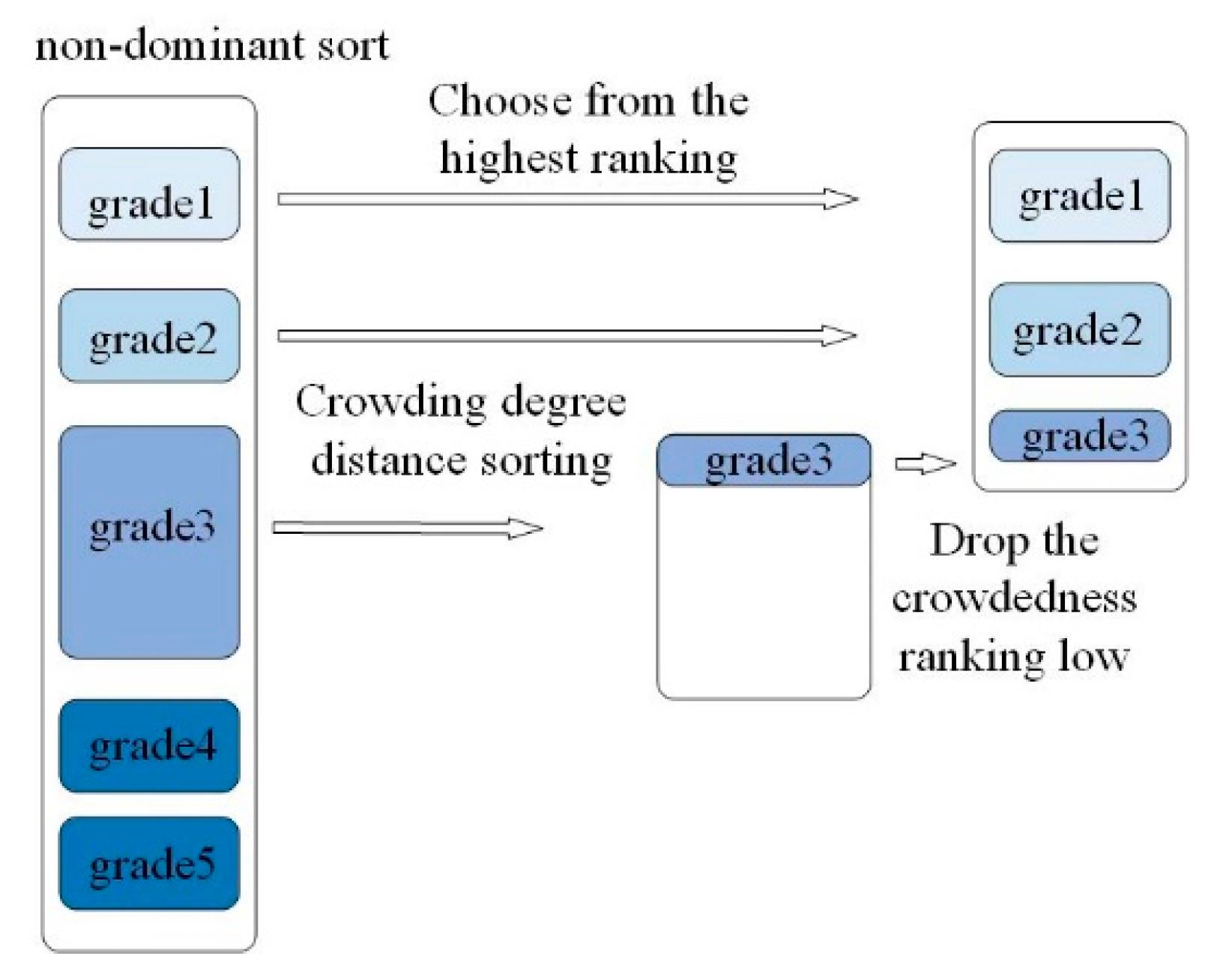
- For non-dominated quick sort, calculate the non-dominated value (Rank value) and crowding degree, as shown in Figure 9. After the non-dominant sorting is completed, the better individuals such as grade 1 and grade 2 are selected as the next-generation parent population. In order to keep the same number as the original parent population in the new-generation parent population, grade 3 cannot all be put into the new generation parent population. Then, the individuals of grade 3 are sorted by crowding degree, and the one with higher crowding degree is selected as the next-generation parent population.
- The tournament selects parents suitable for breeding. Each child needs to have two parents (Parent1 and Parent2), and the parents are selected through a competition in the parent population. Two individuals are randomly selected from the parent population and then compared. First, compare according to rank. If the rank is different, take the individual with better rank. If the rank is the same, compare the crowding degree (Crowding), and take the individual with better crowding distance. Finally, Parent1 is filtered out. The same method filters out Parent2;
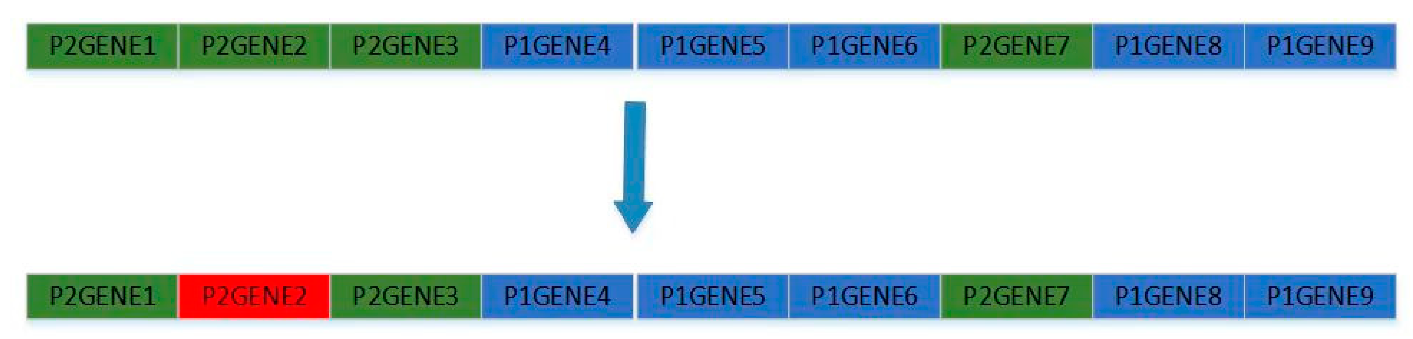
- Genetic operation, crossover, and mutation operation. The crossover process is to extract the genes of the selected individuals and mix them. The crossover operation is realized by partial matching crossover (PMX). During the mutation process, a random gene is selected and modified. The specific operation process is shown in Figure 10 and Figure 11. The gene points for genetic manipulation are customer points and charging stations; select and delete charging stations that do not conform to the charging station insertion strategy, and finally form a solution set.
- Form the progeny population, combine the parent and progeny populations and calculate the fitness of the combined population;
- For non-dominated quick sort, calculate the non-dominated value rank value and crowding degree of the combined population;
- For elite selection, select the top N individuals in the combined population to form a new population. The parent population and the progeny population are synthesized into a population according to the following rules to generate a new parent population from the population. According to the order of Pareto level from low to high, put the population of the same level into the parent population until a certain level of individuals of this level cannot be put into the parent population, arrange the individuals in this layer from large to small according to the degree of crowding, and put them in turn. Enter the parent population until it reaches the parent population;
- End the iteration if the set maximum number of iterations is reached; otherwise, return to Step 6.
3. Results
3.1. Parameter Settings
3.2. Example Test
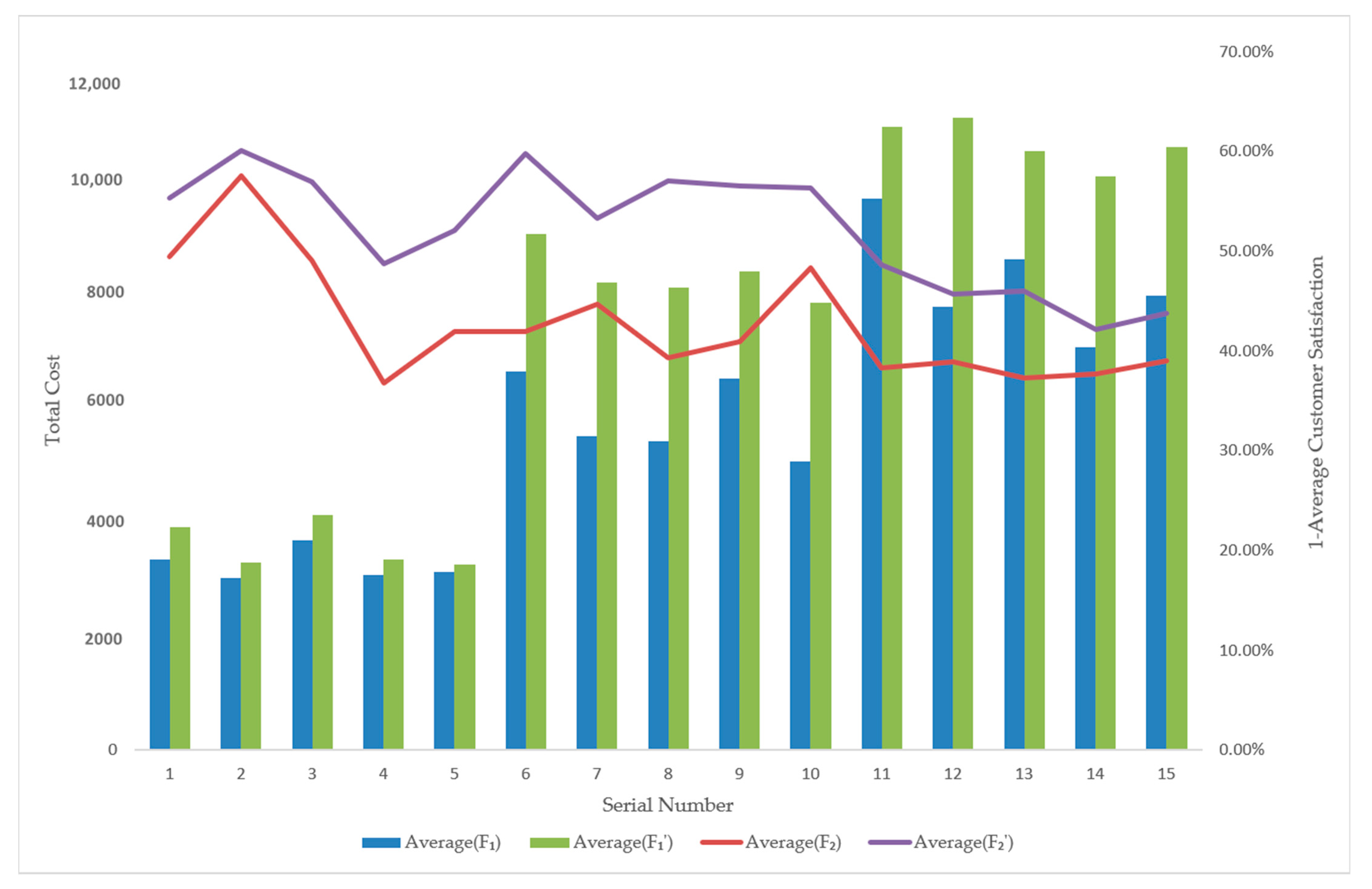
- It can be concluded from the test table of calculation example results in Table 4 and Figure 12, Figure 13 and Figure 14 that there is a contradiction between customer satisfaction and distribution enterprise cost. Random generation of 20, 40, or 80 customer points of each pick and delivery volume occurs. When the goods carried by the vehicles meet the vehicle load, the vehicles return to any distribution center. In order to compare the impact of the number of vehicles on the objective function, the number of vehicles in the fleet is assumed to be 2, 5, and 6. In the 20-customer example, each car needs to satisfy 10 customers on average. In the case of 40 customers, each car needs to satisfy 8 customers on average, and in the case of 80 customers, each car needs to satisfy 13 customers on average. In the CSPS-NSGA II solution results, 46.67% of the examples have customer satisfaction of more than 60%, 46.67% of the examples have customer satisfaction of more than 50%, and 6.67% of the examples have customer satisfaction of more than 40%. The average cost of each calculation case of 15 calculation cases is CNY 2018.33, which can improve the average customer satisfaction by 22.94%.
- It can be seen from the comparison of 20 customer examples, 40 customer examples, and 80 customer examples in Table 4 that with the increase in customer points, the distribution distance will increase. The distribution path with too long a distance will lead to the frequent charging and discharging of electric vehicles in charging stations, resulting in redundant formal costs and charging costs. Therefore, the number of fuel vehicles will gradually increase, while the number of electric vehicles will gradually decrease.
- This can be seen from the comparison of 20 customer examples and 40 customer examples as well as 20 customer examples and 80 customer examples in Table 4. The number of distribution vehicles increases with the number of customer points, and the total cost of distribution increases with the number of customer points and the number of distribution vehicles. The more customer points in the driving path of each vehicle, the more difficult the time window of customer demand is to meet and the lower the customer satisfaction is. The greater the number of customers, the greater the cost of enterprise distribution.
- From the 40-customer example in Table 4 and the 80-customer examples: when the distribution task for the number of electric vehicles in the mixed team uses more fuel, then average customer satisfaction is low, because the electric car in the process of long-distance distribution frequently enters into the charging station, and charging time influences the customer satisfaction.
3.3. Economic Benefits
4. Discussion
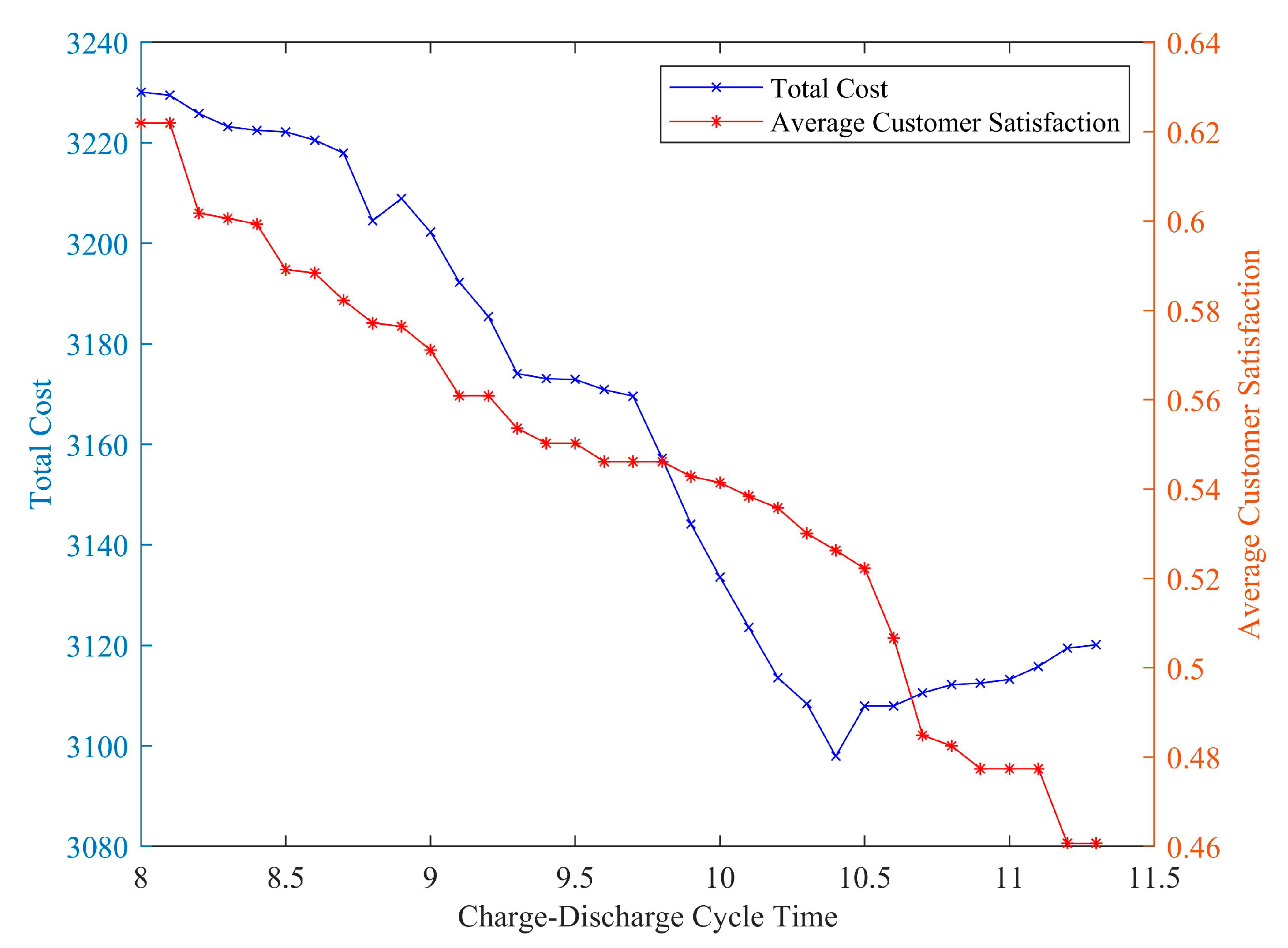
4.1. Electric Vehicle Charge and Discharge Cycle Time
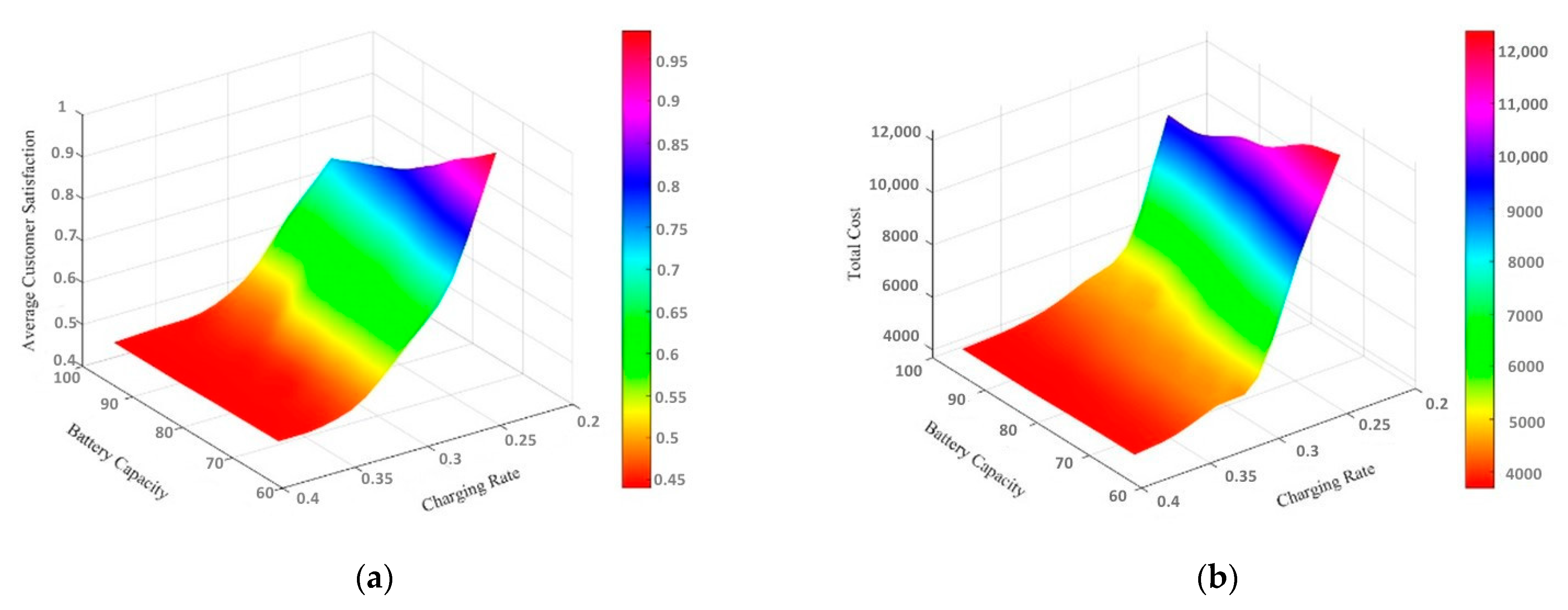
4.2. Battery Capacity and Charging Rate
5. Conclusions
Author Contributions
Funding
Institutional Review Board Statement
Informed Consent Statement
Acknowledgments
Conflicts of Interest
References
- Bruglieri, M.; Mancini, S.; Pezzella, F.; Pisacane, O. A path-based solution approach for the green vehicle routing problem. Comput. Oper. Res. 2019, 103, 109–122. [Google Scholar] [CrossRef]
- National Bureau of Statistics. Statistical Bulletin of the People′s Republic of China on National Economic and Social Development in 2021. 2021. Available online: http://www.stats.gov.cn/tjsj/zxfb/202202/t20220227_1827960.html (accessed on 19 March 2022).
- Teoh, T.; Kunze, O.; Teo, C.C.; Wong, Y.D. Decarbonisation of urban freight transport using electric vehicles and opportunity charging. Sustainability 2018, 10, 3258. [Google Scholar] [CrossRef] [Green Version]
- Islam, M.A.; Gajpal, Y.; ElMekkawy, T.Y. Mixed fleet based green clustered logistics problem under carbon emission cap. Sustain. Cities Soc. 2021, 72, 103074. [Google Scholar] [CrossRef]
- Xv, X.; Jiang, M.; Deng, Y. Dynamic vehicle routing problem with simultaneous pickup and delivery in collaborative distributi-on under demand concurrent. J. Manag. Sci. China 2021, 24, 106–126. [Google Scholar]
- Rahman, I.; Vasant, P.M.; Singh, B.S.M.; Abdullah-Al-Wadud, M.; Adnan, N. Review of recent trends in optimization techniques for plug-in hybrid, and electric vehicle charging infrastructures. Renew. Sust. Energ. Rev. 2016, 58, 1039–1047. [Google Scholar] [CrossRef]
- Luo, L.; He, P.; Zhou, S.; Lou, G.; Fang, B.; Wang, P. Optimal scheduling strategy of EVs considering the limitation of battery state switching times. Energy Rep. 2022, 8, 918–927. [Google Scholar] [CrossRef]
- Wang, M. The Electric Vehicle Routing Problem considering Nonlinear Battery Depreciation; Tsinghua University: Beijing, China, 2018. [Google Scholar]
- Epding, B.; Ramberg, B.; Jahnke, H.; Stradtmann, I.; Kwade, A. Investigation of significant capacity recovery effects due to long rest periods during high current cyclic aging tests in automotive lithium ion cells and their influence on lifetime. J. Energy Storage 2019, 22, 249–256. [Google Scholar] [CrossRef]
- Zang, Y.; Wang, M.; Qi, M. A column generation tailored to electric vehicle routing problem with nonlinear battery depreciation. Comput. Oper. Res. 2022, 137, 105527. [Google Scholar] [CrossRef]
- Pelletier, S.; Jabali, O.; Laporte, G. The electric vehicle routing problem with energy consumption uncertainty. Transp. Res. B-Meth. 2019, 12, 225–255. [Google Scholar] [CrossRef]
- Ferro, G.; Paolucci, M.; Robba, M. Optimal Charging and Routing of Electric Vehicles with Power Constraints and Time-of-Use Energy Prices. IEEE Trans. Veh. Technol. 2020, 69, 14436–14447. [Google Scholar] [CrossRef]
- Hou, D.; Fan, H.; Ren, X. Multi-Depot Joint Distribution Vehicle Routing Problem Considering Energy Consumption with Time-Dependent Networks. Symmetry 2021, 13, 2082. [Google Scholar] [CrossRef]
- Li, J.; Wang, F.; He, Y. Electric Vehicle Routing Problem with Battery Swapping Considering Energy Consumption and Carbon Emissions. Sustainability 2020, 12, 10537. [Google Scholar] [CrossRef]
- You, G. Sustainable vehicle routing problem on real-time roads: The restrictive inheritance-based heuristic algorithm. Sustain. Cities Soc. 2022, 79, 103682. [Google Scholar] [CrossRef]
- Gan, J.; Zhan, X.; Li, J. Electric refrigerate vehicle routing optimization with time windows and energy consumption. Ind. Eng. Manag. 2022, 27, 204–210. [Google Scholar]
- Hornstra, R.P.; Silva, A.; Roodbergen, K.J.; Coelho, L.C. The vehicle routing problem with simultaneous pickup and delivery and handling costs. Comput. Oper. Res. 2020, 115, 10485. [Google Scholar] [CrossRef]
- Foroutan, R.A.; Rezaeian, J.; Mahdavi, I. Green vehicle routing and scheduling problem with heterogeneous fleet including reverse logistics in the form of collecting returned goods. Appl. Soft Comput. 2020, 94, 106462. [Google Scholar] [CrossRef]
- Jia, Y.; Zeng, W.; Xing, Y.; Yang, D.; Li, J. The Bike-Sharing Rebalancing Problem Considering Multi-Energy Mixed Fleets and Traffic Restrictions. Sustainability 2021, 13, 270. [Google Scholar] [CrossRef]
- Al-dal’ain, R.; Celebi, D. Planning a mixed fleet of electric and conventional vehicles for urban freight with routing and replacement considerations. Sustain. Cities Soc. 2021, 73, 103105. [Google Scholar] [CrossRef]
- Malladi, S.S.; Christensen, J.M.; Ramirez, D.; Larsen, A.; Pacino, D. Stochastic fleet mix optimization: Evaluating electromobility in urban logistics. Transp. Res. E-Log 2022, 158, 102554. [Google Scholar] [CrossRef]
- Yu, V.F.; Jodiawan, P.; Gunawan, A. An Adaptive Large Neighborhood Search for the green mixed fleet vehicle routing problem with realistic energy consumption and partial recharges. Appl. Soft Comput. 2021, 105, 107251. [Google Scholar] [CrossRef]
- Hou, K.; Fan, H.; Ren, X. Vehicle routing optimization of multi-center hybrid fleet joint distrubution under time-varying road network. J. Dalian Marit. Univ. 2022, 48, 11–22. [Google Scholar]
- Li, Y.; Zhang, P.; Wu, Y. Vehicle routing problem with mixed fleet of conventional and electric vehicles. J. Syst. Manag. 2020, 29, 522–531. [Google Scholar]
- Wang, J.; Wang, H.; Chang, A.; Song, C. Collaborative Optimization of Vehicle and Crew Scheduling for a Mixed Fleet with Electric and Conventional Buses. Sustainability 2022, 14, 3627. [Google Scholar] [CrossRef]
- Shojaei, M.; Fakhrmoosavi, F.; Zockaie, A.; Ghamami, M.; Mittal, A.; Fishelson, J. Sustainable Transportation Networks Incorporating Green Modes for Urban Freight Delivery. J. Transp. Eng. A-Syst. 2022, 148, 04022028. [Google Scholar] [CrossRef]
- Rinaldi, M.; Picarelli, E.; D′Ariano, A.; Viti, F. Mixed-fleet single-terminal bus scheduling problem: Modelling, solution scheme and potential applications. Omega 2020, 96, 102070. [Google Scholar] [CrossRef]
- Lu, T.; Yao, E.; Zhang, Y.; Yang, Y. Joint Optimal Scheduling for a Mixed Bus Fleet Under Micro Driving Conditions. IEEE Trans. Intell. Transp. Syst. 2021, 22, 2464–2475. [Google Scholar] [CrossRef]
- Zhao, P.; Liu, F.; Guo, Y.; Duan, X.; Zhang, Y. Bi-Objective Optimization for Vehicle Routing Problems with a Mixed Fleet of Conventional and Electric Vehicles and Soft Time Windows. J. Adv. Transp. 2021, 2021, 9086229. [Google Scholar] [CrossRef]
- Ren, X.; Huang, H.; Feng, S.; Liang, G. An improved variable neighborhood search for bi-objective mixed-energy fleet vehicle routing problem. J. Clean. Prod. 2020, 275, 124155. [Google Scholar] [CrossRef]
- LI, D.; Chen, Y.; Zhang, Z. A branch-and price algorithm for electric vehicle routing problem with time windows and mixed fleet. Syst. Eng.-Theory Pract. 2021, 41, 995–1009. [Google Scholar]
- Rafael, B.; Balazs, K.; Bo, E. Energy consumption estimation integrated into the electric vehicle routing problem. Transp. Res. D Transp. Environ. 2019, 69, 141–167. [Google Scholar]
- Zhao, H.; Zhang, C. An online-learning-based evolutionary many-objective algorithm. Inf. Sci. 2020, 509, 1–21. [Google Scholar] [CrossRef]
- Pasha, J.; Dulebenets, M.A.; Fathollahi-Fard, A.M.; Tian, G.D.; Lau, Y.Y.; Singh, P.; Liang, B.B. An integrated optimization method for tactical-level planning in liner shipping with heterogeneous ship fleet and environmental considerations. Adv. Eng. Inform. 2021, 48, 101299. [Google Scholar] [CrossRef]
- Dulebenets, M.A.; Pasha, J.; Kavoosi, M.; Abioye, O.F.; Ozguven, E.E.; Moses, R.; Boot, W.R.; Sando, T. Multiobjective optimization model for emergency evacuation planning in geographical locations with vulnerable population groups. J. Manag. Eng. 2020, 36, 04019043. [Google Scholar] [CrossRef]
- Dulebenets, M.A. A Delayed Start Parallel Evolutionary Algorithm for just-in-time truck scheduling at a cross-docking facility. Int. J. Prod. Econ. 2019, 212, 236–258. [Google Scholar] [CrossRef]
- Rabbani, M.; Oladzad-Abbasabady, N.; Akbarian-Saravi, N. Ambulance routing in disaster response considering variable patient condition: NSGA-II and MOPSO algorithms. J. Ind. Manag. Optim. 2022, 18, 1035. [Google Scholar] [CrossRef]
- Verma, S.; Pant, M.; Snasel, V.A. Comprehensive Review on NSGA-II for Multi-Objective Combinatorial Optimization Problems. IEEE Access 2021, 9, 57757–57791. [Google Scholar] [CrossRef]
- Montoya, A.; Gueret, C.; Mendoza, J.E.; Villegas, J.G. The electric vehicle routing problem with nonlinear charging function. Transp. Res. B-Meth. 2017, 103, 87–110. [Google Scholar] [CrossRef] [Green Version]
- Zhang, D.; Qiao, X.; Xiao, B.; Wang, R.; Mao, C. Multi-objective vehicle routing optimization based on low carbon perspective and random demand. J. Railw. Sci. Eng. 2021, 18, 2165–2174. [Google Scholar]
- National Energy Administration, Gasoline for Motor Vehicles, GB 17930-2016. 2016. Available online: http://openstd.samr.gov.cn/bzgk/gb/newGbInfo?hcno=C45A3554980A86E41F5AA4C6F3D48DC1 (accessed on 19 March 2022).
- Zheng, Y.; Li, F.; Dong, J.; Luo, J.; Zhang, M.; Yang, X. Optimal Dispatch Strategy of Spatio-temporal Flexibility for Electric Vehicle Charging and Discharging under “EVs-traffic-distribution” Model. Autom. Electr. Power Syst. 2022, 1–27. Available online: http://kns.cnki.net/kcms/detail/32.1180.TP.20220430.0926.002.html (accessed on 27 April 2022).


| Variable | Significance |
|---|---|
| represents all nodes in the city logistics network, | |
| represents N distribution centers in the collection | |
| represents that there are H customer points in the set, | |
| it means that there are charging stations in set | |
| it means that there are cars in the set | |
| represents that there are delivery tasks in the set | |
| refers to the maximum energy consumption of vehicle d to complete the task | |
| refers to the d-th vehicle of node | |
| refers to all nodes that the vehicle needs to visit one by one | |
| refers to the speed of the vehicle from to | |
| refers to the maximum load of the vehicle | |
| refers to the distance between node and node | |
| refers to the self-weight of the d-th vehicle at node | |
| refers to the cargo weight of the d-th vehicle from node | |
| refers to customer h delivery demand | |
| refers to customer h recycling demand | |
| refers to the fixed cost of the fuel vehicle | |
| refers to the fixed cost of the electric vehicle | |
| refers to the unit energy consumption cost of the fuel vehicle | |
| refers to the unit energy consumption cost of the electric vehicle | |
| refers to the penalty cost of delaying service per unit time | |
| refers to the waiting cost of advance service per unit time | |
| refers to the start time of the task | |
| refers to the time when the vehicle arrives at the node | |
| refers to EV travel time in task | |
| refers to the time window of the task , | |
| refers to the optimal arrival time window of the customer’s expected task , | |
| refers to the service time required by node A in task | |
| represents vehicle from node to node | |
| represents vehicle is electric vehicle | |
| indicates that the vehicle obeys the task | |
| refers to customer h satisfaction | |
| refers to the charging cost per unit time | |
| refers to the depreciation cost of battery cycles | |
| refers to the battery depth of discharge depreciation cost | |
| refers to the number of times the vehicle enters the charging station | |
| refers to the minimum state of charge of an electric vehicle battery | |
| q | refers to the total number of charge and discharge cycles of the electric vehicle d |
| refers to the fixed constant related to the type of battery | |
| refers to the depth of battery discharge | |
| refers to the charging and discharging cycle time before the electric vehicle is put on hold | |
| refers to the fuel vehicle energy consumption conversion factor | |
| refers to the electric vehicle energy consumption conversion factor | |
| refers to emissions per unit of energy consumption, | |
| refers to the tax on emissions | |
| g | refers to the acceleration of gravity |
| refers to the slope between different roads | |
| is the coefficient of rolling resistance | |
| is the air resistance coefficient | |
| A | is the windward area of the vehicle |
| is the air density | |
| is the road elevation between nodes |
| Variable | Significance | Variable | Significance |
|---|---|---|---|
| 1 CNY/kWh | |||
| 50 CNY/t | |||
| 2.5 t | |||
| 5 t, 6 t, 7 t | |||
| 15 CNY/h | |||
| 8 CNY/h | |||
| 1/3.212 × 104 | CNY | ||
| 1/3.6 × 103 | CNY | ||
| 10 h | 6.26 CNY/L | ||
| q | 2000 times | 0.6226 CNY/kWh |
| Algorithm Parameters | Population Size | Number of Iterations | Crossover Rate | Variation Rate |
|---|---|---|---|---|
| parameter value | 50 | 100 | 0.8 | 0.2 |
| Examples | ) | ) | ) | ) | ) | ) | V(o1–o2) | |
|---|---|---|---|---|---|---|---|---|
| tc1c20s3ct1 | 1/2 | 2947 | 3640.18 | 3269.06 | 32.22% | 63.67% | 49.44% | 1–1/0–2 |
| tc1c20s3ct3 | 1 | 2637.53 | 3298.03 | 2966.34 | 38.18% | 75.95% | 57.50% | 1–1 |
| tc1c20s3ct4 | 1/2 | 3063.85 | 4549.22 | 3607.94 | 25.03% | 67.37% | 49.04% | 1–1/0–2 |
| tc2c20s3cf0 | 1/2 | 2290.20 | 3797.38 | 3004.58 | 19.79% | 52.20% | 36.75% | 1–1/0–2 |
| tc2c20s3ct0 | 1/2 | 2538.96 | 3666.40 | 3063.36 | 17.49% | 62.47% | 41.98% | 1–1/0–2 |
| tc1c40s5cf1 | 5 | 5183.36 | 6362.64 | 6504.83 | 38.33% | 51.59% | 41.89% | 0–5 |
| tc1c40s5ct1 | 4/5 | 4422.73 | 7076.05 | 5389.16 | 34.33% | 59.61% | 44.63% | 1–4/0–5 |
| tc2c40s5cf2 | 5 | 4465.91 | 7889.84 | 5309.37 | 34.68% | 44.96% | 39.32% | 0–5 |
| tc2c40s5cf3 | 6 | 4586.78 | 8177.96 | 6373.17 | 32.29% | 55.68% | 40.92% | 0–5 |
| tc2c40s5ct2 | 4/5 | 4134.77 | 6381.82 | 4964.62 | 36.41% | 63.15% | 48.28% | 1–4/0–5 |
| tc1c80s8cf2 | 2 | 9401.53 | 9635.98 | 9480.44 | 37.44% | 39.28% | 38.26% | 4–2 |
| tc2c80s8cf3 | 1/2 | 6408.35 | 8555.70 | 7609.75 | 34.42% | 48.30% | 38.85% | 5–1/4–2 |
| tc2c80s8cf4 | 2 | 7263.14 | 9886.94 | 8432.65 | 36.01% | 38.91% | 37.29% | 4–2 |
| tc2c80s8ct3 | 2/3 | 5313.15 | 9032.42 | 6915.66 | 28.25% | 53.81% | 37.65% | 4–2/3–3 |
| tc2c80s8ct4 | 2 | 7378.83 | 10360.54 | 7810.11 | 32.95% | 44.90% | 38.98% | 4–2 |
| Pareto Points | Optimized Path | ||
|---|---|---|---|
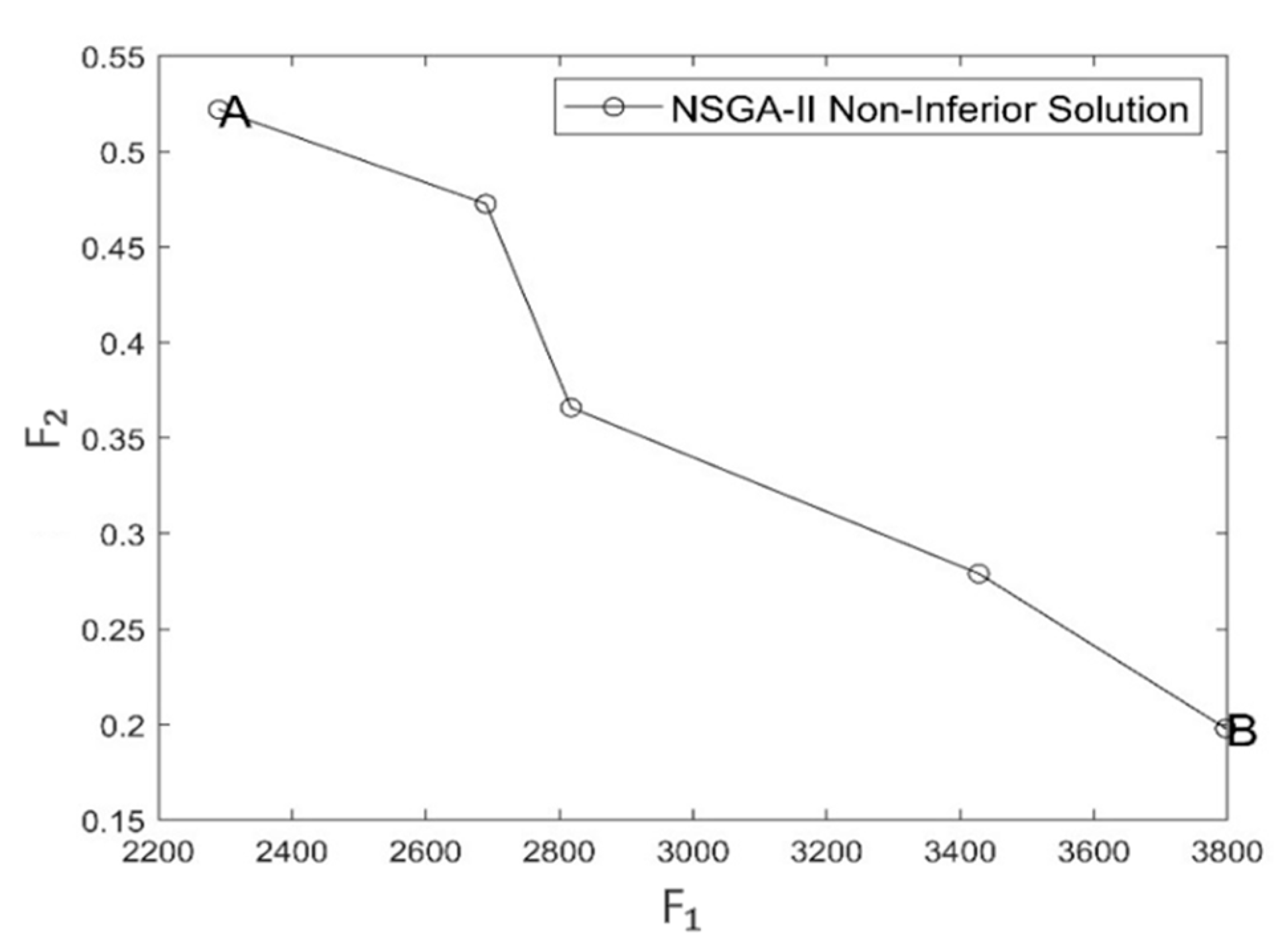
| A | 1-6-9-8-20-23-12-21-13-16-17-25-19-3; 1-18-14-10-5-7-22-4-15-25-11-3. | 2290.20 | 52.20% |
| B | 2-9-10-11-15-22-18-13-14-19-20-25-4-23-5-3; 2-7-8-12-17-6-21-16-25-2. | 3797.38 | 19.79% |
| C | 1-28-10-17-23-7-16-29-44-14-30-3; 1-26-12-11-13-35-43-46-41-5-1; 3-4-9-25-38-21-44-31-22-2; 3-20-27-18-37-15-24-36-33-3; 2-8-6-34-42-40-39-46-32-19-3. | 4134.77 | 63.15% |
| D | 2-28-5-23-14-43-16-46-17-31-34-3; 1-40-9-11-13-30-45-21-32-2; 1-42-27-12-25-38-15-41-48-19-33-1; 2-22-4-37-26-24-18-44-20-8-1; 3-35-7-10-39-29-44-6-36-1. | 6381.82 | 36.41% |
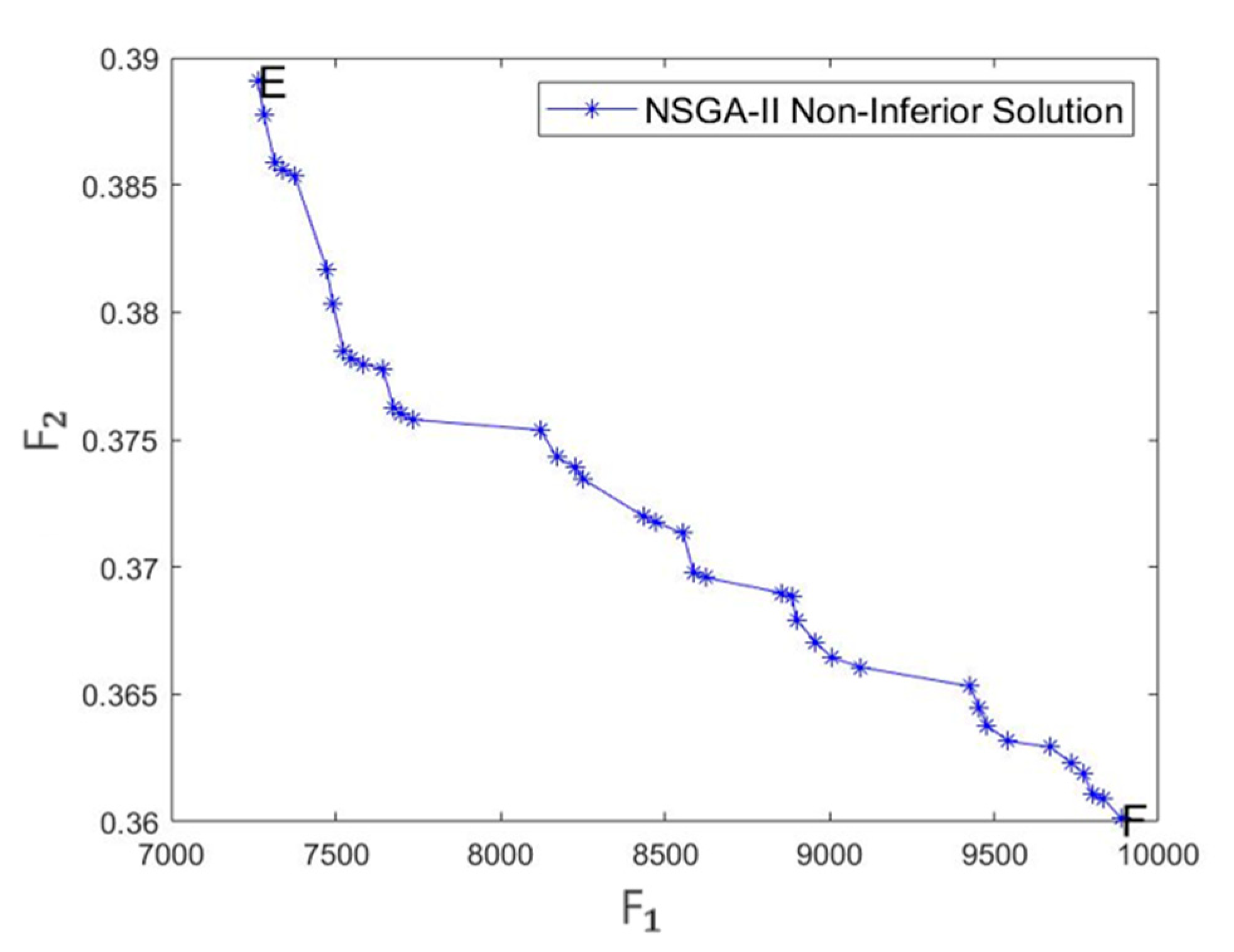
| E | 3-26-63-72-27-82-30-75-81-25-42-49-31-58-24-57-33-79-2; 1-50-15-18-14-56-16-28-78-60-62-65-7-40-59-1; 2-54-76-61-77-5-86-23-43-1; 2-41-9-20-74-21-19-69-70-52-48-73-64-55-46-67-45-2; 3-29-17-10-22-53-12-66-36-44-6-32-80-37-39-38-83-13-3; 1-8-47-11-35-71-68-4-86-34-51-1. | 7263.14 | 38.91% |
| F | 3-26-38-72-27-82-30-75-81-25-42-49-31-58-24-57-33-79-2; 1-50-15-18-14-56-16-28-78-60-62-52-7-40-37-1; 2-54-76-61-68-5-86-23-83-1; 2-41-9-20-74-77-19-69-70-65-48-73-64-55-46-67-45-2; 3-29-17-10-22-53-12-63-36-44-6-32-13-59-39-66-80-43-3; 1-8-47-11-35-71-21-4-86-34-51-1. | 9886.94 | 36.01% |
| Serial Number | Examples | ||||
|---|---|---|---|---|---|
| 1 | tc1c20s3ct1 | 3269.06 | 49.44% | 3833.16 | 55.31% |
| 2 | tc1c20s3ct3 | 2966.34 | 57.50% | 3217.70 | 60.07% |
| 3 | tc1c20s3ct4 | 3607.94 | 49.04% | 4028.61 | 56.98% |
| 4 | tc2c20s3cf0 | 3004.58 | 36.75% | 3267.36 | 48.71% |
| 5 | tc2c20s3ct0 | 3063.36 | 41.98% | 3191.42 | 52.09% |
| 6 | tc1c40s5cf1 | 6504.83 | 41.89% | 8865.70 | 59.73% |
| 7 | tc1c40s5ct1 | 5389.16 | 44.63% | 8034.17 | 53.29% |
| 8 | tc2c40s5cf2 | 5309.37 | 39.32% | 7938.73 | 57.07% |
| 9 | tc2c40s5cf3 | 6373.17 | 40.92% | 8223.69 | 56.50% |
| 10 | tc2c40s5ct2 | 4964.62 | 48.28% | 7678.90 | 56.28% |
| 11 | tc1c80s8cf2 | 9480.44 | 38.26% | 10705.35 | 48.58% |
| 12 | tc2c80s8cf3 | 7609.75 | 38.85% | 10863.44 | 45.65% |
| 13 | tc2c80s8cf4 | 8432.65 | 37.29% | 10287.50 | 46.00% |
| 14 | tc2c80s8ct3 | 6915.66 | 37.65% | 9861.88 | 42.18% |
| 15 | tc2c80s8ct4 | 7810.11 | 38.98% | 10355.19 | 43.79% |
Publisher’s Note: MDPI stays neutral with regard to jurisdictional claims in published maps and institutional affiliations. |
© 2022 by the authors. Licensee MDPI, Basel, Switzerland. This article is an open access article distributed under the terms and conditions of the Creative Commons Attribution (CC BY) license (https://creativecommons.org/licenses/by/4.0/).
Share and Cite
Li, M.; Shi, Y.; Zhu, B. Research on Multi-Center Mixed Fleet Distribution Path Considering Dynamic Energy Consumption Integrated Reverse Logistics. Sustainability 2022, 14, 6613. https://doi.org/10.3390/su14116613
Li M, Shi Y, Zhu B. Research on Multi-Center Mixed Fleet Distribution Path Considering Dynamic Energy Consumption Integrated Reverse Logistics. Sustainability. 2022; 14(11):6613. https://doi.org/10.3390/su14116613
Chicago/Turabian StyleLi, Mengke, Yongkui Shi, and Bobin Zhu. 2022. "Research on Multi-Center Mixed Fleet Distribution Path Considering Dynamic Energy Consumption Integrated Reverse Logistics" Sustainability 14, no. 11: 6613. https://doi.org/10.3390/su14116613
APA StyleLi, M., Shi, Y., & Zhu, B. (2022). Research on Multi-Center Mixed Fleet Distribution Path Considering Dynamic Energy Consumption Integrated Reverse Logistics. Sustainability, 14(11), 6613. https://doi.org/10.3390/su14116613