Abstract
In the face of demand disruptions, dual-channel supply chains (SCs) that lack resilience may be more vulnerable. Reaching moderate SC resilience through coordination is essential for dealing with disruptions. This paper investigates the operation management of a dual-channel fresh-food SC (FSC) under disruption. The centralized and decentralized decision models propose joint quality efforts based on the consideration of quality preference and loss. From the perspective of SC resilience, we analyze how SC members can optimally make price, quality, and quantity decisions resiliently and robustly under the disruption of quality preference. The results show that (1) no matter the kind of decision model, considering quality preference disruptions can significantly increase the SC profit; (2) there is a resilience range in decisions with the influence of the disruption cost. The original optimal decisions in the resilience range are robust and sustain SC performance without change; and (3) the disruption significantly impacts offline channel retailers, who are at a disadvantage when competing with online channels. A centralized decision model can achieve higher profits and quality levels in response to demand disruptions. This paper extends the concept of resilience to the FSC and provides suggestions for fresh-food enterprises to conduct quality efforts and cope with demand interruption.
1. Introduction
Recently, e-commerce has gradually changed the consumption patterns of consumers and the sales methods of fresh-food enterprises. Especially since the beginning of the COVID-19 pandemic, buying fresh food through online channels has become a mainstream method [1]. More and more fresh-food enterprises have adopted the combination of online and offline dual-channel supply chains (SCs) as their essential strategy. However, fresh food is significantly different from other packaged foods, as it is perishable, and a large volume will be lost in the operation of the SC [2]. Statistical analysis revealed that the loss of fresh food in China has reached 25–35%, whereas it is 15% in developed countries [3]. Furthermore, spoilage in fresh food can easily be perceived by consumers and affect their purchasing decisions. According to a report by iResearch (https://report.iresearch.cn/report/202105/3776.shtml, accessed on 15 May 2021), consumers’ preferences for price and quality are important factors affecting the operation of the fresh-food SC (FSC) with the improvement in consumption level [4]. It is worth noting that the consumers in first- and second-tier cities with a solid demand for fresh-food e-commerce are more sensitive to quality. Sustainable SC management is becoming an emerging consensus in various industries and enterprises [5].
In today’s dynamically changing SC environment, the various challenges of the FSC were analyzed by Yadav et al. [6], and these authors divided these challenges into four categories: sustainability, food waste, food safety and security, and miscellaneous challenges. With limited resources, meeting this exponentially growing demand for food and maintaining sustainable practices in the FSC is a huge challenge [7]. Sustainability challenges are mainly reflected in efforts to maintain freshness, weaker environmental regulation and enforcement, etc. [8]. Food waste and loss are often seen as a problem, accounting for one-third of total food production, and are related to poor storage facilities, cold chain deficiencies, etc. [9]. The challenges of food safety and security mainly come from consumer awareness, etc. [10]. Miscellaneous challenges manifest in many ways due to the complexity of the SC. Recent incidents of cybersecurity breaches highlight that cybersecurity is now a SC issue, creating new challenges for SC management [11]. Furthermore, challenges such as uncertainty, supply and demand mismatch, poor irrigation, and drought management exist in each stage of the SC, hindering the development of FSC [12].
Industry 4.0 is a continuous trend of using information technology to promote industrial transformation, including advanced technologies such as big data management, blockchain technology (BCT), the Internet of Things (IoT), etc. [13,14]. In recent years, these technologies have started to gain popularity in SC innovation and have led to the formation of SC 4.0 [15]. Gayialis et al. [16] proposed a BCT-based approach to ensure the origin, quality, and authenticity of wines and spirits. Kechagias et al. [17] applied systems thinking to the pharmaceutical industry, using Ventana’s simulation system dynamics method to simulate and optimize the quality control process. To drive digital transformation, many information systems have been established in urban distribution systems [18], maritime network security systems [19], etc. Technological advances have facilitated the sustainable development of the FSC. Track and trace facilities with new technology have been applied to efficiently check product quality and inventory levels, resulting in improved performance and less damage [20].
The FSC also calls for flexibility in terms of response capacity and improvement in SC resilience against disruptions due to changing customer preferences [21]. Risk management is vitally important to the FSC compared to a typical SC. Fresh food has three unique properties: perishability, a long production cycle, and seasonal production. Perishability means that the FSC is time-critical and requires quality effort from all SC members [22]. Due to the perishability of fresh food, their quality issues are closely watched by consumers. The current FSC faces challenges, including growing food demand and consumer preferences for food safety and quality [6]. The disruption of consumer quality preference has become a significant problem in the operation management of the FSC [23,24]. For example, the 2019 African Swine Fever epidemic severely affected pork quality, causing pork consumption to plummet. There have been frequent occurrences of unsellable fruits in recent years, mainly fruits that do not meet consumer quality preference [25].
Resilience is essential for effective SC risk management and aims to produce or foster moderate resilience in the SC to deal with the risk of disruption [26]. Because fresh food consumption is year-round, whereas production is seasonal and long-term, there is an imbalance between product supply and demand cycles. Long supply lead times limit the possibility of quick replacements in the case of a shortage [27]. A resilient FSC can quickly return to its original state or move to a new, more desirable state after a disruption [28]. Therefore, it is necessary to apply the concept of resilience during the decision-making stage to planning for the harvesting, storage, and transport of fresh produce. SC coordination is an effective means to build moderate resilience in the SC [29]. This involves designing an appropriate coordination incentive mechanism based on factors such as logistics, capital flow, and information flow among SC members. Regarding the research on the contract selection of coordinated SC coordination, a typical example is a revenue sharing contract. The revenue sharing provided by the contract demonstrates a good incentive and pre-control effect on the quality input and level of the SC [30]. Compared with the no-contract situation, the contract can achieve a “win-win” situation for revenue and quality and resilience to disruption [31].
This paper investigates the price and quality policy in a dual-channel FSC under the disruption of consumer quality preference and attempts to answer the following research questions:
- How can we formulate resilient price and quality strategies in a fresh-food dual-channel SC under the disruption of quality preference?
- What would be the implications for supply chain performance considering quality preference disruptions?
- How will a resilient supply chain strategy be affected, and how will it differ from a non-resilient decision?
To solve the above problems, this paper investigates an online and offline dual-channel FSC composed of one manufacturer and one retailer. Rahmani et al. [32] considered this type of SC structure as the basic dual-channel SC model, which could be regarded as the baseline for studying SCs with multiple manufacturers and multiple retailers. First, we introduce consumers’ quality preference into the market demand function. Regarding the quality of fresh food, we consider the joint efforts of manufacturers and retailers and the loss of quality. For quality preference disruption, we design the corresponding disruption cost to obtain each profit function. Second, based on the Stackelberg game, we solve the centralized and decentralized decision-making modes’ optimal price, quality, and quantity strategies. In various disruption scenarios, we analyze the impact of quality preference disruption on profits. In view of the inability to provide specific profit distribution among members under centralized decision-making, a revenue sharing contract is proposed to realize SC coordination. Finally, we explore the scope for resilient SC decision-making and corresponding management recommendations.
The contributions of this paper are as follows: first, we consider the impact of consumer quality preference disruption on market demand. Most FSC decision studies focus only on the effects of sales price and quality, ignoring the disruption of quality preference. Second, this paper investigates a dual-channel FSC with a comparative analysis of optimal price, quality, and quantity decisions in baseline and disruption scenarios. For the disruption situation under centralized decision-making, a revenue-sharing contract is proposed for SC coordination. Finally, differing from previous studies on SC resilience that focus on qualitative research, we quantitatively analyze how to make resilient production decisions under the disruption of quality preferences.
The structure of this paper is as follows: Section 2 provides a literature review. Section 3 establishes the dual-channel food SC model, setting the demands, disruption costs, and profits. Section 4 and Section 5 are divided into two cases, baseline and disruption, to solve the optimal price and quality strategies of the centralized and decentralized decision model. Section 6 proposes and proves propositions related to the operation management of the FSC based on the model. Section 7 proposes a revenue-sharing contract model. Section 8 describes and discusses the resilience range of the dual-channel FSC through numerical simulation. Finally, Section 9 summarizes the whole work and reaches conclusions. All proofs are in Appendix A.
2. Literature Review
2.1. Dual-Channel FSC
The dual-channel FSC could be mainly divided into three models: the manufacturer dual-channel, the retailer dual-channel, and the mixed dual-channel model [24]. In the manufacturer dual-channel model, the manufacturer plans to establish an additional direct online channel in addition to the retailer’s traditional offline sales channel [33]. The manufacturer first receives the order placed by the consumer on the online sales channel and then directly distributes the fresh food to the consumer from the production base [34]. For example, Pagoda and Dolly Farm have adopted the manufacturer dual-channel model. The retailer dual-channel model means that the manufacturer sells fresh food wholesale to the retailers who open online channels [35]. Typical companies using this model are Hema Fresh, Super Species, etc. As for the mixed dual-channel model, it can be seen as a combination of the above two models, where both manufacturers and retailers are developing online channels [36]. This paper will mainly study the manufacturer dual-channel model.
2.2. Consumer Preference
The price preference has always been the main foothold of scholars’ research. Still, quality preference cannot be ignored in the operation of FSC to improve consumers’ quality awareness. Yang et al. [36] developed FSC under three sales modes, considering the quality preference. Cai et al. [37] only considered the impact of quality preference on the SC through third-party logistics of fresh food. Lambertini [38] considered both quality and price preference. Ma et al. [39] proposed a three-echelon FSC considering freshness-keeping preference and effort with asymmetric information. Zhang et al. [40] found that the high sensitivity of quality preference can improve the preservation effect of the SC to a certain extent, thereby reducing product loss. Zhang et al. [41] argued that a price discount contract with an effort adjustment strategy or cost-sharing strategy can coordinate the SC. In addition, some scholars have considered low-carbon preference based on quality preference [24]. Therefore, due to the quality loss of fresh food, the models that only consider price preference are inaccurate, and quality preference should be added to improve SC performance.
2.3. Quality Effort
Among different supply chain entities, there are two main ways to improve quality efforts [25]. For manufacturers, these are mainly reflected in quality improvement efforts in production. Some fresh-food enterprises build their production bases to produce and process high-quality products or purchase high-quality upstream products with the help of a professional buyer team by establishing high-quality standards, such as Dingdong, Yiguo, etc.
Retailers mainly focus on freshness-keeping efforts at the sales stage. Hema and Super Species improve the freshness of their products by investing in complete cold chain logistics and fresh-food warehouses. In addition, well-equipped freshness-keeping equipment in stores and delivery services within 30 min improve product quality.
However, many scholars have focused on manufacturers’ efforts, ignoring the retailer’s efforts. Wu et al. [42] considered an outsourcing logistics channel whose quality effort and price affect the fresh food’s sellable quantity and quality. Zheng et al. [43] designed a freshness-keeping cost-sharing contract and revenue-sharing contract. Chuang and Wu [44] proposed an integrated supplier–retailer SC model considering quality effort with an asymmetric tolerance design and allowable shortage. As fresh food is perishable, it is vital to improve fresh-food quality from the production and distribution sides. Furthermore, considering the joint quality efforts of manufacturers and retailers in the SC decision model has important implications for the quality of fresh food instead of available manufactured products.
2.4. SC Disruption
This study believes that SC disruption refers to the state in which SC operation deviates from expectations due to external or internal disruption factors, thereby bringing various risks to enterprises. This could lead to other SC disruptions, mainly in terms of demand, consumer preference, price, cost, etc.
Huang et al. [45] were the first to study disruption management in a dual-channel SC. They focused on the impact of production cost disruptions on the SC but only considered the effect of price factors on demand. Subsequently, Huang et al. [46] explored in great depth the situation where demand and cost are disturbed at the same time. Giri et al. [47] focused on coordination under demand and supply disruption in a three-layer SC. Huang et al. [48] studied the price and inventory policy of the food SC with production disruption and controllable deterioration. Wan et al. [23] analyzed the coordination of a fresh agricultural product SC when the production cost and the loss rate are disrupted simultaneously. Mondal et al. [49] adopted interval a type-2 Pythagorean fuzzy set to describe uncertainty in SC risk management. Ali et al. [50] proposed a multi-objective mixed-integer nonlinear SC coordination model by studying the complexities of spoilage, transportation, demand uncertainty, price volatility, and transportation inefficiency. Many scholars have also studied SC disruptions under mixed uncertainty during the COVID-19 pandemic [51].
Based on the above research, the current research mainly focuses on the disruption of total market demand or cost. There are still few studies on the disruption of consumer preference. Rahmani et al. [32] explored a dual-channel SC affected by price and green level under demand disruption. However, the disruption of consumers’ green preference was ignored. Wang et al. [52] studied a single-channel SC situation in response to consumer preference disruptions. Si et al. [53] found an optimization SC strategy and analyzed the channel competition effect under the disruption of coupon promotion input and consumer preference. Therefore, it is necessary to conduct further research on the disruption of quality preference.
2.5. SC Resilience
SC resilience refers to the ability of the SC to return to its original state or an ideal state after a disruption, which mainly includes four dimensions: reliability, robustness, recovery, and reconfigurability [54]. Leat et al. [28] argued that supply chain resilience improved through horizontal collaboration among producers and cooperation with processors and retailers. Ivanov et al. [55] examined the range of disruption-based changes in supply structures and parameters needed to remain resilient for the dairy supply chain in Australia. Aviral et al. [56] defined the robustness of the SC based on four aspects, optimized the structure of the SC from the perspective of the emergency inventory, and provided research ideas for SC optimization under moderate flexibility. Wicaksono et al. [57] improved the resilience of food supply chains by applying the development of quality function deployment methods. Liu et al. [58] concluded that SC resilience is the key for cross-border e-commerce companies to gain a competitive advantage continuously. Few studies have quantitatively obtained how a dual-channel fresh-food supply chain makes resilient decisions in response to disruptions.
2.6. Research Gap
For the FSC, many studies have been conducted on inventory management, pricing, and ordering strategies. The literature related to this field is compared in Table 1.

Table 1.
Literature comparison.
According to the existing literature, this paper combines the channel characteristics and pricing strategies of the dual-channel FSC under quality preference disruption and quality effort based on SC resilience. The previous literature tends to focus on price preference in the research on consumer preference. However, for fresh food, quality preference is also significant to the operation of the supply chain and should be taken into account. In the research in this field, the research on disruption is mainly on demand and production cost, and few studies have considered the disruption of quality preference. In terms of quality effort, more effort is considered for a single member, and less is considered for joint efforts. Most studies on SC resilience focus on qualitative evaluation, factor analysis, etc. Few studies have considered how to achieve SC resilience from the production decision (price, quality, quantity, etc.).
Therefore, the innovation of this paper is mainly in the research into a dual-channel FSC, focusing on the perspective of quality management while considering quality preference, quality preference disruption, and quality joint effort. In addition to deciding on the optimal price, quality, and quantity, this paper focuses on decision-making with resilience and studies its influencing factors, application scope, and corresponding management decisions.
3. Model Description
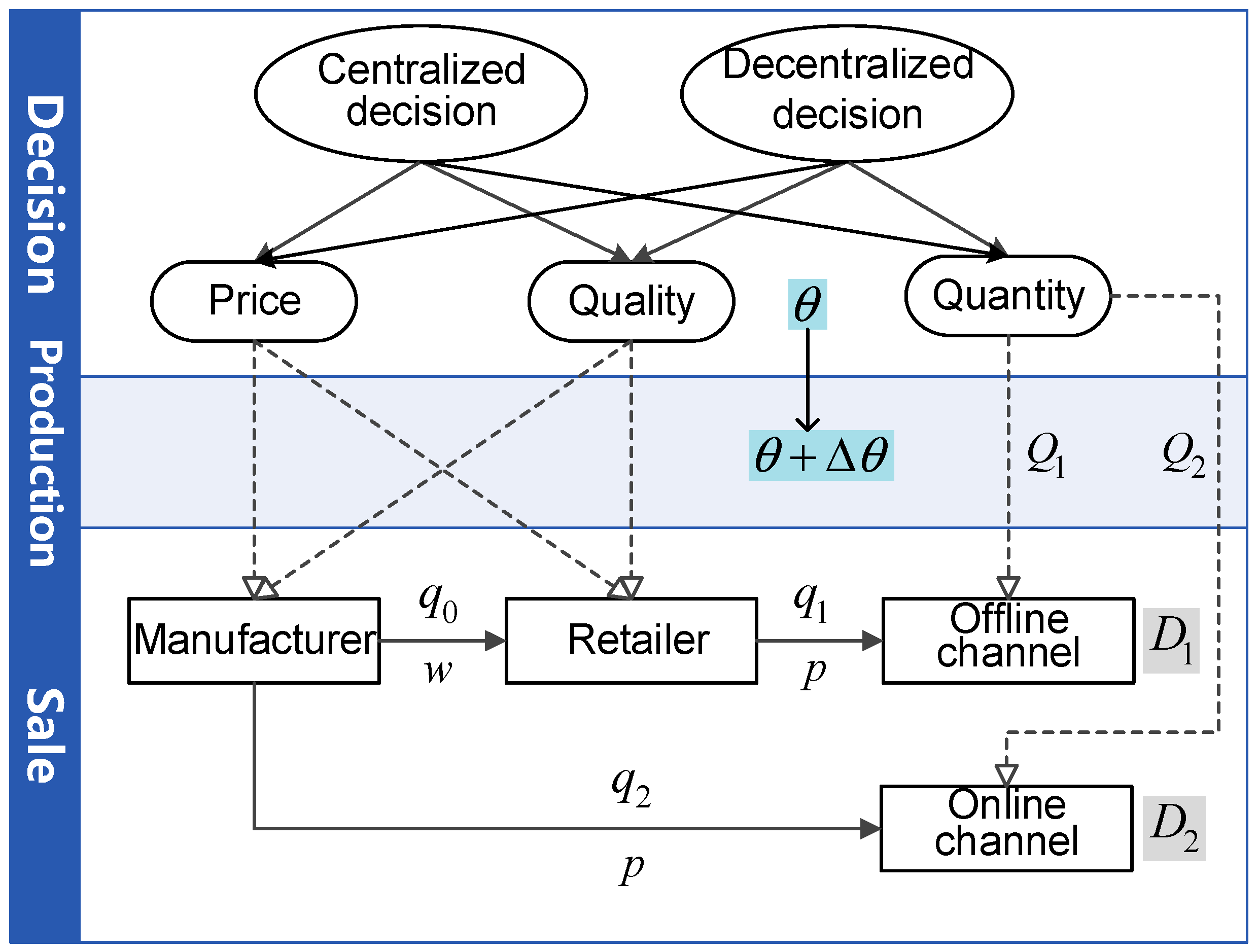
As shown in Figure 1, the FSC model is divided into three stages: decision, production, and sales. The time proportion of the three stages is uneven, the production of fresh food takes the longest, and each type of fresh food generally has a corresponding suitable planting season. In the decision stage, centralized and decentralized decision-making are the two most typical decision-making methods in dual-channel SCs [33]. It is assumed that the SC will be divided into two decision-making methods to determine the price, quality, and quantity of fresh food. The production decisions are based on the original market demand and consumer quality preference. During the production stage, the changes in consumer quality preference may cause demand disruptions, so the original decisions may not adapt to the new quality preferences in the sales stage. Thus, due to the disruption of quality preference, it is possible that the original decision will be suboptimal. Inevitably, the disruption will generate additional disruption costs, which will reduce the profit of the SC.
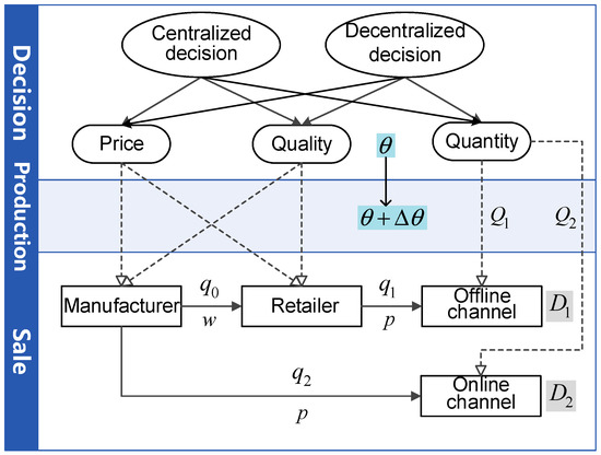
Figure 1.
The SC model for fresh food.
To facilitate unified expression, the notations are defined in Table 2.
Table 2.
Symbol description.
The model assumptions are as follows:
- The market information of the manufacturer and retailer is symmetrical, and their risk preference is assumed to be neutral and entirely rational. In this study, the FSC targets one kind of fresh food and operates for a cycle. It is assumed that the manufacturer has the ability to meet market demand and the retailer does not have inventory.
- In the literature on operations management and marketing, mainstream scholars have proposed linear demand assumptions for price and non-price variables [60,61]. To simplify the model and simple operation, we assume that the main factors influencing channels’ demand are price and quality when consumers purchase fresh food.
- Investment in quality efforts is a one-time expense. For the convenience of calculation, it is assumed that the manufacturer’s production cost is 0. This assumption is similar to Li et al. [62].
In the decision stage, the consumer’s quality preference is assumed to be , whereas the quality preference may change and become in the sales stage. When , it means that the current quality of fresh food conforms to the consumer preference trend. In contrast, when , it means that consumer preference is decreasing. Based on [63,64], adopting a consistent pricing strategy in dual-channel can alleviate the conflict of competition between the channels. Similar practices are seen in companies such as Hema Fresh and Super Species [36].
The demands of online and offline channels are defined as follows:
The total demand of all channels in the centralized decision is defined as follows:
It is assumed that the manufacturer produces fresh food of the same and launches it on the market. Both channels will make quality efforts to increase sales, so that the quality levels when they reach consumers are and . Following Krishnan et al. [65], the setting of the fresh food quality effort level and wastage rate under quality effort is expressed as: , where the constraints are and . The value range of this function is . When , it means that the fresh food has decayed and cannot be sold, whereas there is almost no change in the quality level of fresh food when . According to the marginal beneficial characteristics of investment, the quality effort level function is a concave function. It is positively correlated with the cost but stabilizes after reaching a certain degree, expressed as: [66,67].
In the sales stage, the actual demand for fresh food may be different from the original production quantity . Due to demand disruptions, the SC will incur disruption costs: when , the SC has to increase order quantity or other methods to meet additional demand, resulting in costs such as being out of stock. When , the SC will incur inventory costs, processing costs caused by deterioration, etc. Similar to Wang et al. [52] and Qi et al. [68], the model will set and to represent the disruption cost when demand rises or falls. Suppose satisfies , , thus the whole additional cost of the demand disruption can be expressed as:
where means .
Due to the perishability of fresh food and the high quality requirements, the main costs of manufacturers and retailers in various channels are caused by quality efforts. Moreover, the sales cycle is short, and the inventory cost expenditure is mainly in the performance improvement of the inventory facility. Therefore, only the cost of quality improvement will be considered in this model, whereas the cost of production and operation will be ignored in each channel.
When dual-channel sales are at , the demand is and , respectively, and the related quality improvement costs and demand disruption costs are assumed. The profit function is:
For the model to be established, it supposes that all the parameters are positive. In order to signify the demand disruption case, we use the current notations with wavy lines.
4. Centralized Decision Model
In the centralized decision model, the manufacturer and the retailer are treated as a whole system. This means that an overall decision-maker decides the price and quality of fresh food to obtain the total optimal profit.
4.1. Baseline Case
In the baseline case, the original quantity at the time of decision is equal to the actual demand.
Lemma 1.
In a centralized dual-channel FSC without demand disruptions, ifsatisfies the condition ofand, it is a concavefunction with respect to. The optimal sale price andquality effort levelin each channel, respectively, are given by:
The proof is presented in Appendix A.
4.2. Disruption Case
After predicting the actual demand for fresh food, the SC decision-maker should adjust the expected quantity under the original decision to maximize the total profit of the SC system.
Scenario 1: When , then , where is defined in Equation (11). The total profit function of the centralized FSC in this time can be expressed as:
Due to and , needs to conform to the value range of in scenario 1, where .
Scenario 2: When , then . The total profit function of the centralized FSC in this time can be expressed as:
Similarly, needs to conform to the value range of in scenario 2.
Scenario 3: From the range of values derived from scenario 1 and 2, it can be found that there is a value range of between scenario 1 and 2. This shows that when demand disruption occurs and is in a certain range, the difference between and is not large, which may make production decisions resilient. This will be demonstrated later.
Lemma 2.
In the case of demand disruptions, the optimal selling price and the optimal online and offline channel quality level in the centralized dual-channel FSC are determined as follows:
Comparing the obtained under the demand disruption with the under the baseline case, the optimal production quantity of the three scenarios is obtained:
where .
The optimal profits of the SC system under the three disruption scenarios are given by:
5. Decentralized Decision Model
In the decentralized decision-making model, manufacturers and retailers can make independent decisions and seek to maximize their own profits. Due to the unequal competitive position in line with the characteristics of the Stackelberg game, the manufacturer, as the leader of the Stackelberg game, determines the wholesale price and quality effort level first, and then the retailer determines its price as a follower.
In order to ensure that the channel demand and the profits obtained by the manufacturers and retailers are not negative, the following conditions must be met:
5.1. Baseline Case
In the baseline case, there is no demand disruption, and the reverse derivation method will be used to solve the problem of decentralized decision-making. In the solution process, the retailer first determines the offline channel quality effort level, and then the manufacturer decides the price and online channel quality effort level.
Lemma 3.
In a decentralized dual-channel FSC with demand disruptions, ifsatisfies the condition of, and , it is a concave function with respect to . The optimal wholesale price for the retailer, sale price, and quality effort level of manufacturer are given by:
Replacing Equations (24)–(26) into the first-order condition of Equation (7) , we can obtain the optimal quality effort level of a retailer:
The optimal quantity of decentralized decision-making in the baseline case is given by:
Lemma 4.
In the decentralized decision model, in order to satisfy,,, andare solvable. In other words, the consistent pricing strategy would be feasible, and there is an optimal production decision for this problem. The range of consumer preferences is given by:, where,.
From Lemma 4, it can be concluded that in decentralized decision-making, changes in consumer channel preferences will affect the implementation of channel strategies and supply chain members. Therefore, effective market research or big data analysis can help us to understand consumers’ channel preferences promptly and actively adjust market supply and channel strategies to enhance competitiveness.
5.2. Disruption Case
In the case of demand disruptions, according to the actual situation of the fresh food industry, the manufacturer and the retailer will bear the cost of disruption caused by demand disruptions. After demand disruptions occur, the manufacturer and the retailer should adjust their decisions to maximize their profits.
Scenario 1: When , then and , where and are defined in Equations (28) and (29). According to Equation (7), we obtain the first-order condition of as follows:
when the demand disruption occurs and the demand of the product increases, we obtain from Equation (6) and then obtain the first-order partial derivative of with respect to . Therefore, , , and are given by:
where , , , , and . The optimal quality level of manufacturer in this scenario is as follows:
Scenario 2: When , then and . The first-order condition of is given by:
Similarly, , , , and are as follows:
6. Model Analyses
Proposition 1.
In the centralized decision model, when, the optimal decisions regarding price, quality, and quantity are resilient.
Proposition 1 indicates that when is in this interval, the consumer’s quality preference fluctuates little, and there is no need to make changes to the original production decision. When making decisions, SC members should consider future changes in quality preferences so that the quality of fresh food produced can be in the “resilience range”. This could avoid the impact of quality preferences and achieve moderate resilience of the SC. When making decisions, adequate market research should be conducted, not just production but also quality preferences.
Proposition 2.
When,will decrease asincreases, and its maximum value is. When,will increase asdecreases, and its minimum value is.
Proposition 2 reveals that when , the quality of fresh food is very consistent with the current consumer quality preference trend, and the price can be increased appropriately to . When , the quality has seriously deviated from the current consumer quality preference trend, and the price can be appropriately lowered. The minimum is . Therefore, adjusting the price according to the disruption cost can obtain the maximum profit in the SC system as a whole.
Proposition 3.
When,increases monotonically with, and the optimal value is. When,decreases monotonically with, and the optimal value is. is the same.
Proposition 3 shows that in addition to considering , when determining the level of quality effort, it is mainly affected by the loss ratio of fresh food of its own channel , as well as by the influence of the coefficient of quality effort cost in another channel . For centralized decision makers, when considering the quality improvement in the channel, the quality improvement cost of the two channels must be considered at the same time, to avoid channel conflicts and maximize the overall benefits of the SC system.
Proposition 4.
When centralized decision makers make production decisions, considering future consumer quality preference disruptions will provide more benefits than not considering them.
Proof of Proposition 4.
If demand disruptions occur but the centralized decision makers are not aware of them, then we use the production decisions in the baseline case. However, in the actual disruption situation, these decisions may not be optimal. With the change in , the market demand in the sales stage can be expressed as:
Based on the original production decision, the SC system takes into account the additional costs caused by demand disruptions and obtains:
In the actual situation, the profit after considering the demand disruption is compared with the profit without considering the demand disruption, as shown in Table 3. □
Table 3.
Comparison of profits after considering demand disruptions.
Proposition 4 indicates that the quality preference of consumers for fresh food makes manufacturers and retailers more profitable. As a decision-maker in the FSC, it is vitally important to consider the disruption of consumer quality preference. Quality efforts should be aggressively improved to meet consumer quality preference. Regardless of whether it is a positive or negative quality preference disruption, considering the disruption management of quality preferences will increase the profit of the SC.
7. Revenue Sharing Contract
It is well known that the SC profit under the centralized decision model is more than that under the decentralized decision model, but it cannot provide a specific profit distribution between SC members. This paper proposes a revenue sharing contract. The contract parameters are . Manufacturers supply retailers at lower , and may be lower than the cost of production. After the end of the sales period, the retailer needs to share a proportion of the profit with the manufacturer to make up for the loss caused by . Therefore, the profits of manufacturers and retailers are as follows:
The optimal decision under this contract is
Under the revenue sharing contract, to provide the supply chain with Pareto improvement, , , and must be equal to , respectively, and can be obtained simultaneously:
If the designed contract is to be accepted by manufacturers and retailers, both individual rationality and collective rationality must be satisfied. This is to ensure that the profits of the manufacturer and the retailer under the revenue-sharing contract reach Pareto improvement, and so we provide Proposition 5.
Proposition 5.
Under the benefit-sharing contract coordination, there exists, such that. If, then, and all members of the dual-channel SC can achieve Pareto improvement under the revenue sharing contract.
The proof is presented in Appendix A.
Proposition 5 shows that, as long as the profits of the manufacturer and the retailer are not less than their respective profits under decentralized decision making, the dual-channel supply chain can be coordinated under a revenue-sharing contract.
8. Numerical Simulation
To further verify the validity of the model, this paper will use numerical examples for analysis. The parameter setting is combined with the actual investigation of fresh food sales in e-commerce [36,40] and studies on the quality effort and loss of fresh food [25,38]. These parameters express that the current offline sales channels have a slight advantage in channel selection, and consumers are not sensitive to offline prices. According to the constraints of Lemma 1 and Lemma 3, the specific parameter settings are set as shown in Table 4.
Table 4.
Numerical assumptions.
- (1)
- Divided into two cases according to and , with as the independent variable, then , , , , , the trend curve of and versus is shown in Figure 2.
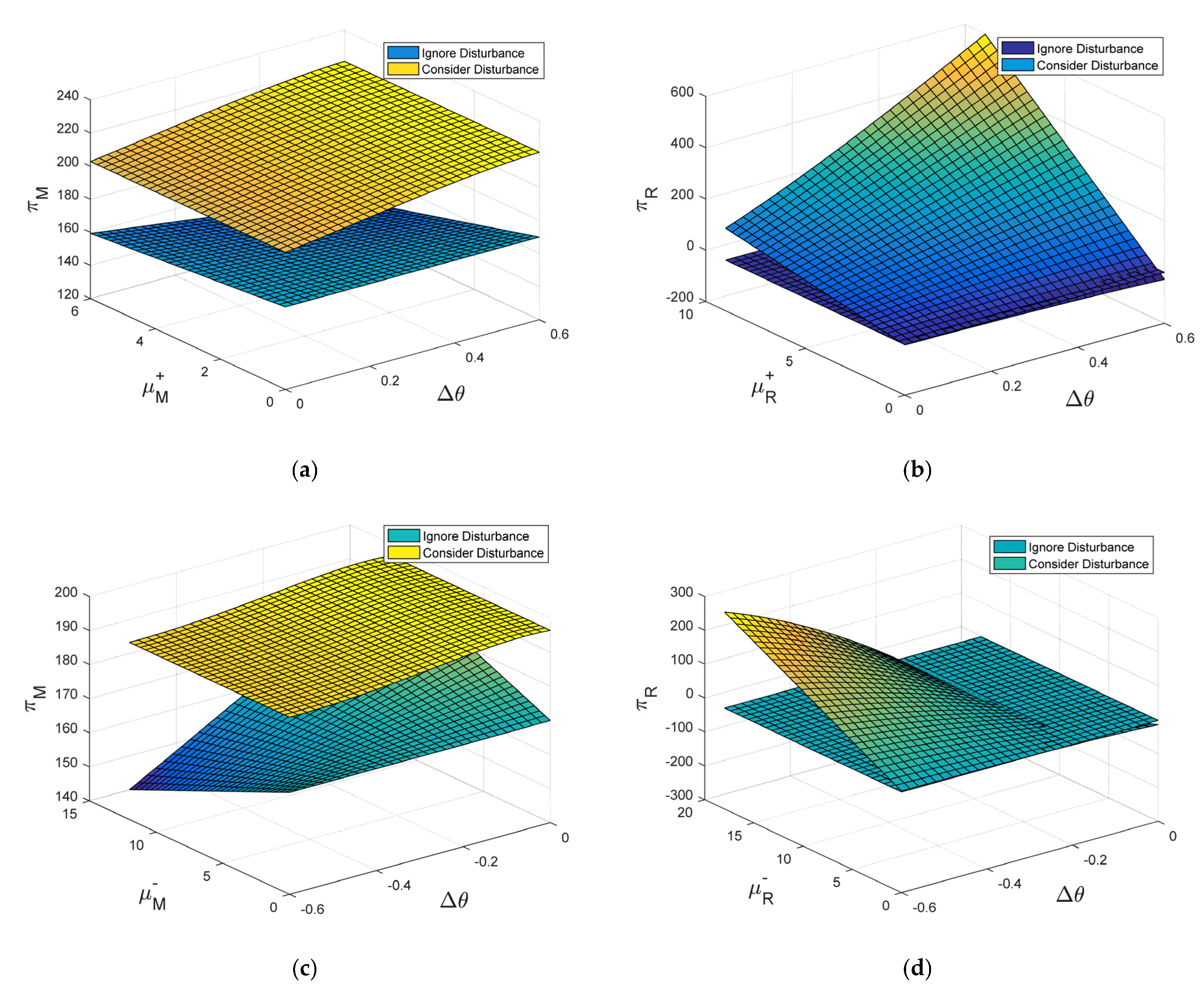
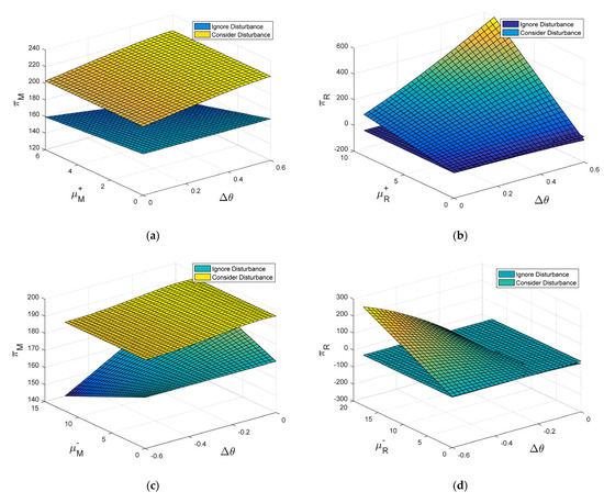 Figure 2. Trend curve of manufacturer and retailer. (a) Trend curve of manufacturer when Δθ > 0. (b) Trend curve of retailer when Δθ > 0. (c) Trend curve of manufacturer when Δθ < 0. (d) Trend curve of retailer when Δθ < 0.
Figure 2 illustrates that regardless of whether it is a manufacturer or a retailer in the decentralized decision model, as long as the disruption of quality preference is considered, it will increase their profit. Among them, when , the improvement in under the original decision does not cause an increase in the profit for the manufacturer, missing the opportunity to improve the quality profit. When , the original decision is more affected by , and the profit of manufacturers considering disruptions will be more stable. This proves that it is necessary to consider the disruption of quality preference, which helps to stabilize the profit and avoid demand disruption.
However, it is worth noting that the Stackelberg game is more beneficial to manufacturers, and retailers will be at a massive disadvantage. Retailer profits plummeted as demand in offline channels plummeted due to disruptions in quality preferences. This may be because offline channel consumers have a more direct perception of the quality of fresh food, and the occurrence of disruptions will cause consumers to stop their consumption behavior. Therefore, retailers should pay more attention to the disruption of quality preferences. While striving to improve quality, new technologies such as BCT are used to improve the traceability and information sharing of fresh products, providing consumers with a tool to easily explore the source of fresh products on their own to create a trusted consumption environment.
- (2)
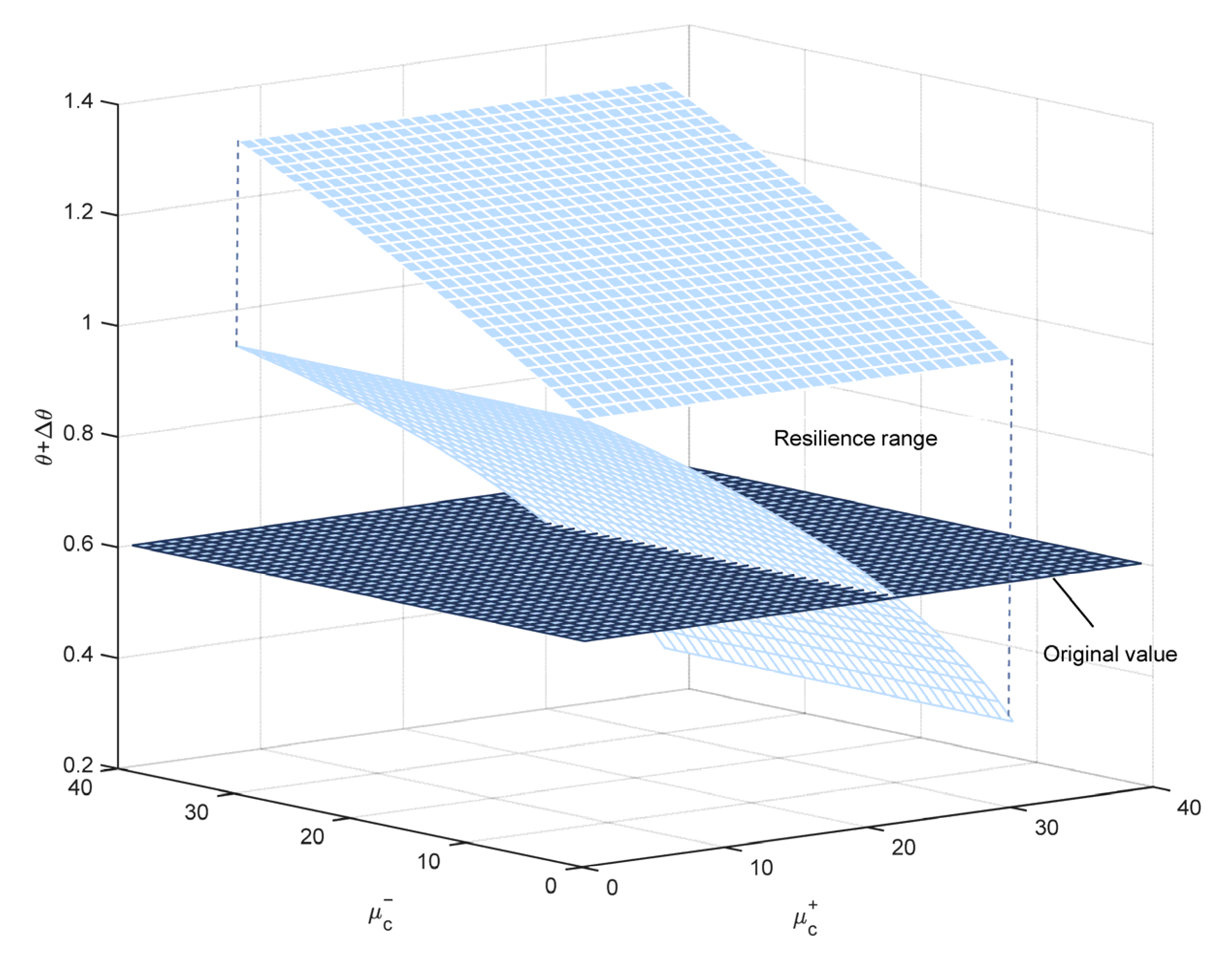
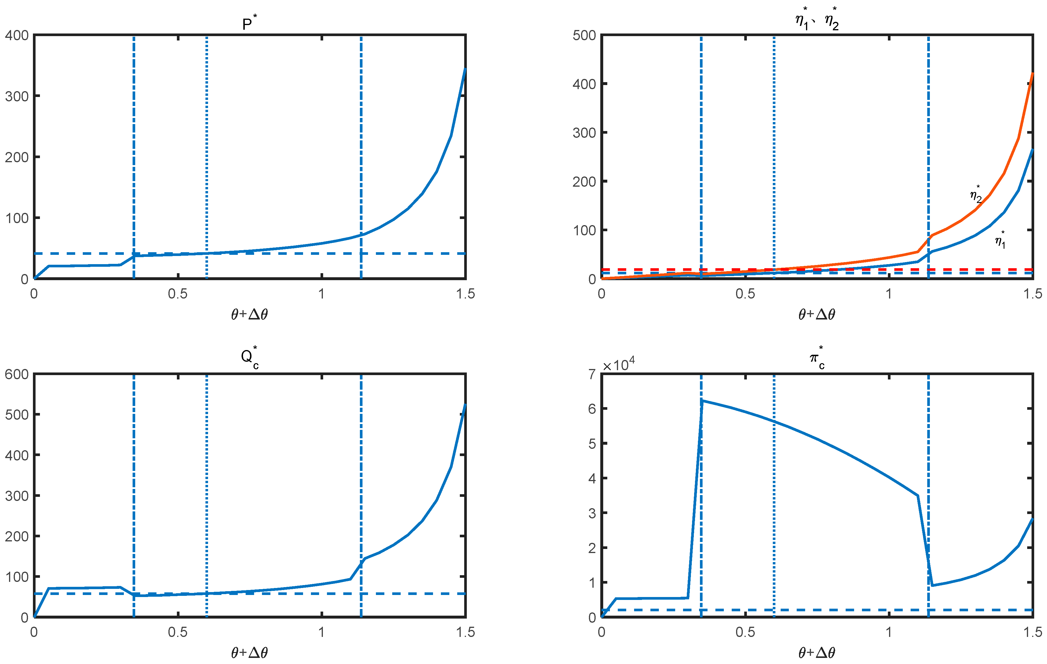
- In the centralized decision model, when , the “resilience range” of is present, as shown in Figure 3. The “resilience range” refers to the range of resilience in decision-making when changes with , . From Figure 3, we can find that the upper and lower limits of the resilience range are mainly affected by and . The increase in the resilience range with is obviously greater than the increase with . Therefore, decision makers need to analyze the cost of disruptions. The resilience range is mainly above the original value of , indicating that when rises, production decisions are more likely to be resilient. Therefore, it is necessary to enhance consumers’ preference for the quality of fresh food through advertising, publicity posters, etc., so as to make the SC income more stable.
 Figure 3. The resilience range of the centralized model.
When is in the resilience range , the change curve of each decision variable is shown in Figure 4. When the disruption is within the resilience range, price, quality, and quantity do not need to change. However, due to the high stock quantity decisions out costing , the profit of the SC will decline. It will also be significantly higher than the profit under the original decision. When the disruption is lower than the resilience range, the price should be lowered to promote sales. In contrast, the quantity needs to be appropriately increased due to the low price advantage. When the disruption is higher than the resilience range, more extraordinary quality efforts are required, but the benefits are far less than the resilience interval decision-making.
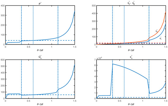
Figure 4.
The change curve of each decision variable when in the resilience range ().
In either case, offline channels have to make more quality efforts than online channels to form SC coordination. This shows that in a centralized decision model, the quality of fresh food that finally reaches consumers through dual channels needs to be differentiated, and appropriate environmental conditions must be maintained in retail stores. For fresh food that needs to be refrigerated, the freshness-keeping temperature must be kept stable to avoid the deterioration of quality due to accidental opening of the freezer, power failure, or other reasons.
- (3)
- In the decentralized decision model, there is also a resilience range similar to Lemma 2, and the solutions of each decision variable are:
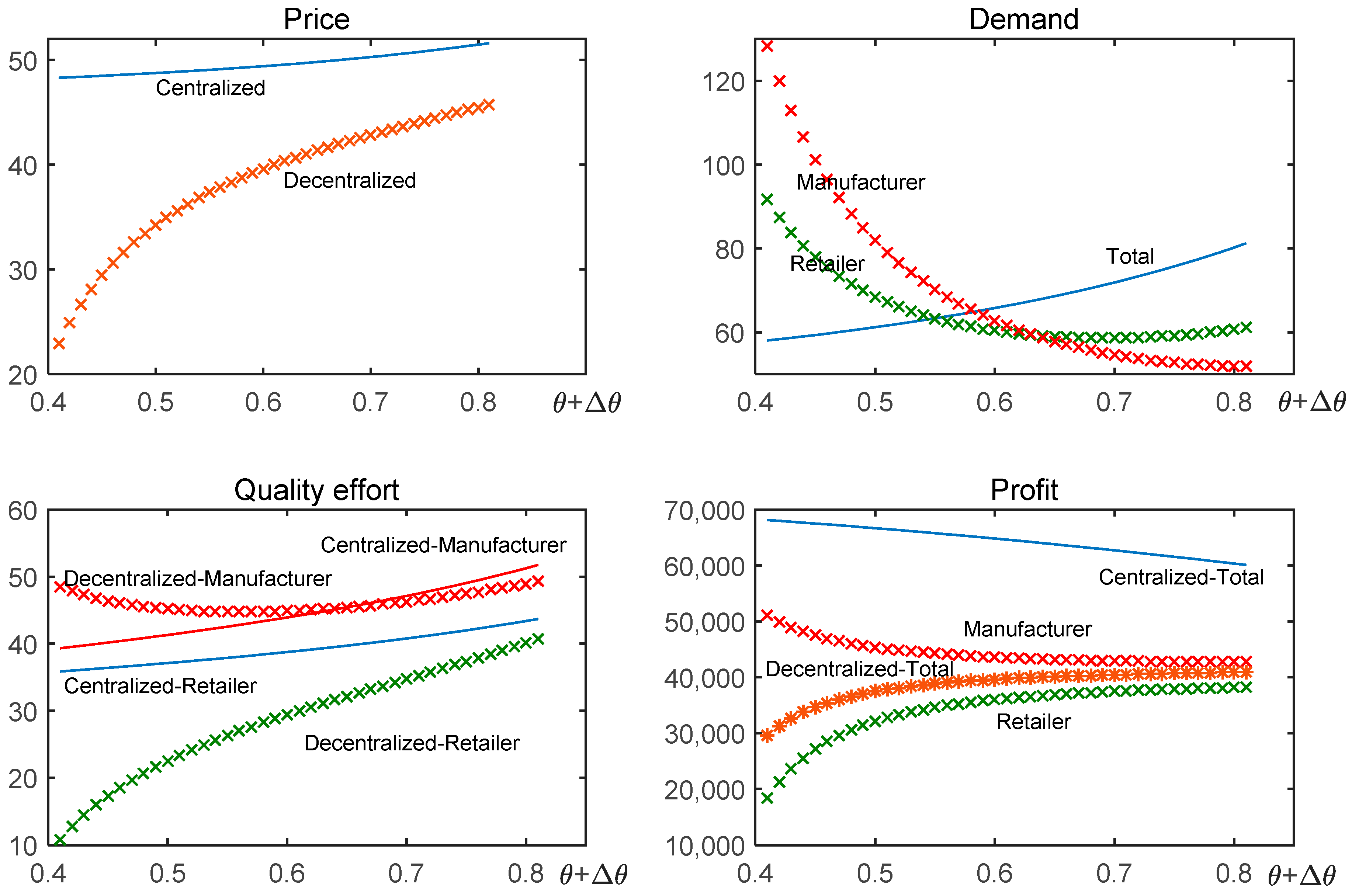
We compare the change curves of the decision variables in the centralized and decentralized model and draw Figure 5. Figure 5 illustrates that when the disruption is in the resilience range, the price of the centralized decision model will be higher than that of the decentralized decision model, and the total profit in the centralized decision model is much higher. This shows that a centralized decision model can effectively alleviate channel conflicts and avoid "price wars" between channels. The higher the consumer’s preference for quality, the greater the quality effort required by retailers. Moreover, prices under a centralized decision model are more stable, reducing the adverse effects of significant price changes on consumers. In addition, the total demand in the centralized decision model is less affected by the disruption. The original decision making is not changed much and can be maintained to reduce decision frequency.
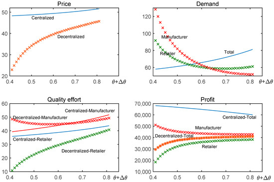
Figure 5.
Change curve of decision variables in centralized and decentralized model in the resilience range.
- (4)
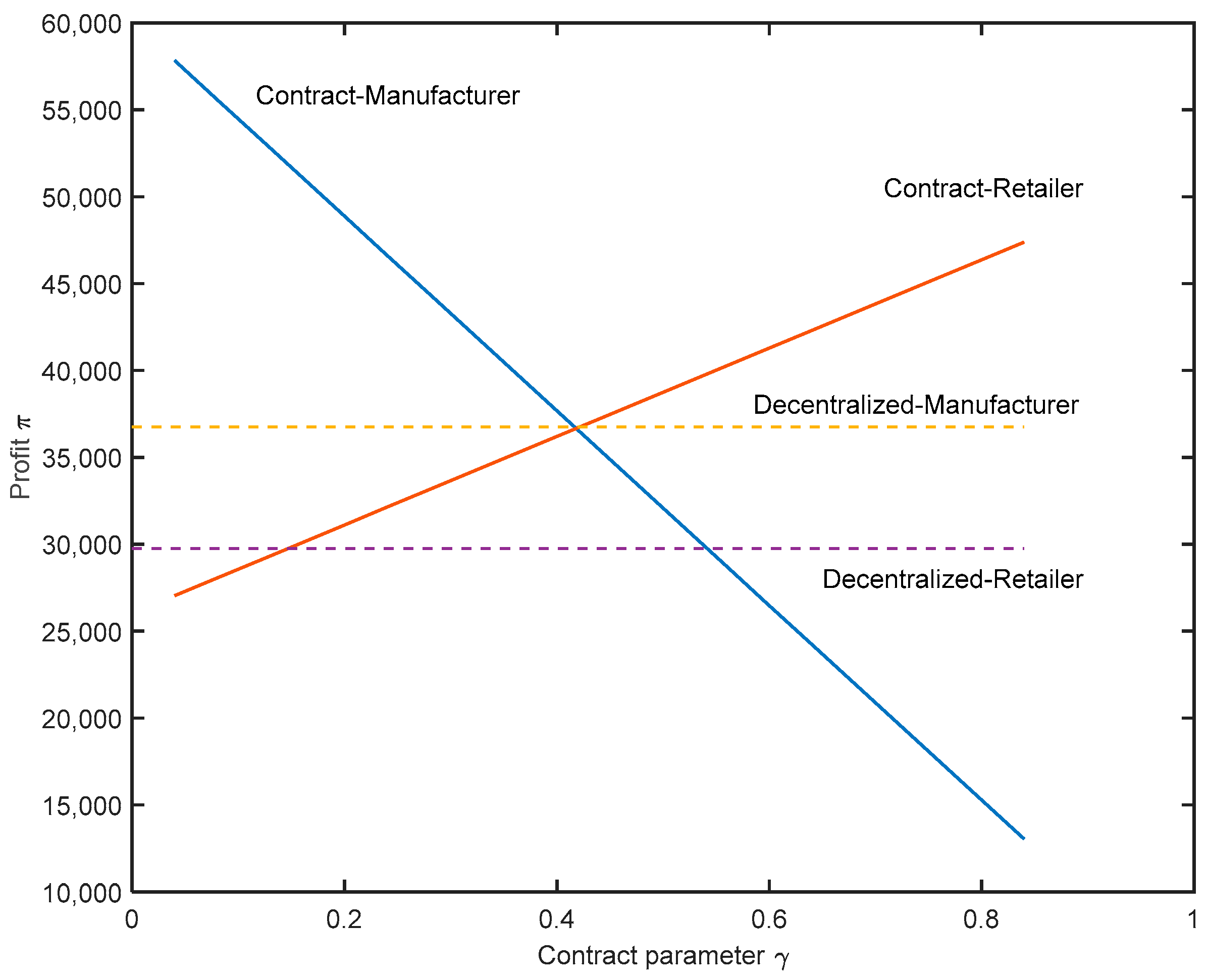
- It can be seen from Figure 6 that when the revenue-sharing contract parameter gradually increases, the manufacturer’s profits decrease, and the retailer’s profits gradually increase. Figure 6 reveals the effect of on the profits of manufacturers and retailers before and after the SC reaches coordination when in a resilience range of . It is calculated that, after contract coordination, when , the manufacturer and retailer achieve Pareto improvement.
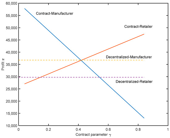 Figure 6. Effect of revenue-sharing contract parameter on profits.
9. Conclusions
This paper conducts modeling on the disruption management problem of the dual-channel FSC based on the perspective of consumer quality preference disruption. First, in view of the baseline case, it studies the price, quality, and production decision-making of the centralized and decentralized decision models. Second, in the case of quality preference disruptions, it divides situations into three scenarios and compared them with the decision-making in the baseline case. We propose a revenue sharing contract to achieve supply chain coordination. Finally, the numerical experiment is used to analyze the profit of SC members under the two decisions and the resilience range generated by the disruption of quality preference.
Based on the above model analysis and numerical simulations, the management insights from this work are summarized as follows:
- When consumer quality preference is slightly disturbed, the FSC’s pricing, quality, and quantity decisions have a range of resilience. The resilience range is mainly affected by disruption cost. Production decisions that establish a resiliency strategy are most effective in mitigating disruption risks. When making decisions, adequate market research should be conducted, not just of production but also quality preferences.
- In response to demand disruptions, a centralized decision model can achieve higher SC profits and quality levels, effectively avoiding channel conflicts and improving the quality of fresh food. The use of revenue sharing contracts can solve the problem of profit disruption in the case of centralized decision-making. However, it is worth noting that the Stackelberg game is more beneficial to manufacturers. Retailers will be at a massive disadvantage and should pay more attention to the disruption of quality preference.
- Regardless of whether it is a centralized or decentralized decision model, considering quality preference disruptions when formulating plans will significantly increase the profit of each member of the SC. Therefore, decision makers must always pay attention to market changes and could actively use big data analysis and other means to identify consumer quality preference.
- In either case, offline channels have to make more quality efforts than online channels to form SC coordination. For fresh food that needs to be refrigerated, the freshness-keeping temperature needs to be kept stable to avoid the deterioration of quality due to accidental opening of the freezer, power failure, or other reasons. While striving to improve quality, new technologies such as BCT are used to improve the traceability and information sharing of fresh food, providing consumers with a tool to easily explore the source of fresh products on their own to create a trusted consumption environment.
It is worth exploring the following points further: (1) the research model in this paper only considers the simple dual-channel approach of a single product, and the SC will be more complicated in actual market conditions. (2) In the disruption management for quality preference, we could consider repurchase contracts, quantity discount contracts, etc., to coordinate the SC. (3) The description of the resilience of the SC is still in the model stage, and its identification, prediction, intervention and other means need to continue to be studied.
Author Contributions
Resources, C.Y.; Supervision, M.D.; Visualization, Y.Z.; Writing—original draft, Z.L.; Writing—review & editing, Q.L. All authors have read and agreed to the published version of the manuscript.
Funding
The work presented in this paper has been supported by grants from National Natural Science Foundation of China (No. 71840003), Natural Science Foundation of Shanghai (No. 19ZR1435600), Humanity and Social Science Planning foundation of Ministry of Education of China (No. 20YJAZH068), Science and technology development project of University of Shanghai for Technology and Science (No. 2020KJFZ038).
Institutional Review Board Statement
Not applicable.
Informed Consent Statement
Not applicable.
Data Availability Statement
Not applicable.
Acknowledgments
The authors are indebted to the reviewers for their constructive comments, which greatly improved the contents and exposition of this paper.
Conflicts of Interest
The authors declare no conflict of interest.
Appendix A
Proof of Lemma 1.
In order to prove concavity, calculate the second-order partial derivatives with respect to , , and and the Hessian matrix of as follows: . Due to , the maximum value of the function needs to satisfy the condition that the second-order main sub-expression of is greater than 0, and the third-order main sub-expression is less than 0. It is a concave function of and has a maximum value. From the first order conditions of Equation (5) ,,, we can obtain Equations (8)–(10), respectively. □
Proof of Lemma 2.
The proof is similar to Lemma 1, and it solves the optimal decision under three scenarios. □
Proof of Lemma 3.
Similar to Lemma 1, calculate the second-order partial derivatives with respect to , and and the Hessian matrix of as follows: . The maximum value of the function needs to satisfy the condition that the first-order main sub-expression is less than 0, the second-order main sub-expression of is greater than 0, and the third-order main sub-expression is less than 0. Therefore, needs to satisfy the condition of , and . From the first order conditions of Equation (6) , , we can obtain Equations (24) and (25), respectively. □
Proof of Lemma 4.
Because there is a constraint Equation (22) on the retailer, incorporate Equations (24) and (25) into and obtain . There is no guarantee that is positive or negative, thus . For the manufacturer, it is necessary to satisfy Equation (23), substitute , to get . □
Proof of Proposition 1.
This can be proved by subtracting Equations (8)–(12) and (17)–(21). □
Proof of Proposition 2.
As has a negative correlation with and is also proved in Lemma 1, it can be concluded that changes with . □
Proof of Proposition 3.
The proof is similar to that of Proposition 2. □
Proof of Proposition 4.
It has been proven in the paper. □
Proof of Proposition 5.
Substituting Equations (45)–(47) into Equations (43) and (44), the optimal profit under the revenue sharing contract can be obtained as . → < 0. That is, is a monotonically decreasing function of , and is a continuous function in (0, 1); ; . Therefore, there is a contract parameter , which leads to being obtained under the revenue sharing contract. The proof for is similar. □
References
- Cang, Y.; Wang, D. A comparative study on the online shopping willingness of fresh agricultural products between experienced consumers and potential consumers. Sustain. Comput. Inform. Syst. 2021, 30, 100493. [Google Scholar] [CrossRef]
- Liu, C.; Chen, W.; Zhou, Q.; Mu, J. Modelling dynamic freshness-keeping effort over a finite time horizon in a two-echelon online fresh product supply chain. Eur. J. Oper. Res. 2021, 293, 511–528. [Google Scholar] [CrossRef]
- Yang, L.; Tang, R.; Chen, K. Call, put and bidirectional option contracts in agricultural supply chains with sales effort. Appl. Math. Model. 2017, 47, 1–16. [Google Scholar] [CrossRef]
- Moon, I.; Jeong, Y.J.; Saha, S. Investment and coordination decisions in a supply chain of fresh agricultural products. Oper. Res. 2018, 20, 2307–2331. [Google Scholar] [CrossRef]
- Mohammed, A.; Harris, I.; Govindan, K. A hybrid MCDM-FMOO approach for sustainable supplier selection and order allocation. Int. J. Prod. Econ. 2019, 217, 171–184. [Google Scholar] [CrossRef]
- Yadav, V.S.; Singh, A.R.; Gunasekaran, A.; Raut, R.D.; Narkhede, B.E. A systematic literature review of the agro-food supply chain: Challenges, network design, and performance measurement perspectives. Sustain. Prod. Consum. 2022, 29, 685–704. [Google Scholar] [CrossRef]
- Yakovleva, N.; Sarkis, J.; Sloan, T. Sustainable benchmarking of supply chains: The case of the food industry. Int. J. Prod. Res. 2012, 50, 1297–1317. [Google Scholar] [CrossRef] [Green Version]
- Mangla, S.K.; Sharma, Y.K.; Patil, P.P.; Yadav, G.; Xu, J. Logistics and distribution challenges to managing operations for corporate sustainability: Study on leading Indian diary organizations. J. Clean. Prod. 2019, 238, 117620. [Google Scholar] [CrossRef]
- Scherhaufer, S.; Moates, G.; Hartikainen, H.; Waldron, K.; Obersteiner, G. Environmental impacts of food waste in Europe. Waste Manag. 2018, 77, 98–113. [Google Scholar] [CrossRef]
- Yadav, V.S.; Singh, A.R.; Raut, R.D.; Cheikhrouhou, N. Blockchain drivers to achieve sustainable food security in the Indian context. Ann. Oper. Res. 2021, 1–39. [Google Scholar] [CrossRef]
- Melnyk, S.A.; Schoenherr, T.; Speier-Pero, C.; Peters, C.; Chang, J.F.; Friday, D. New challenges in supply chain management: Cybersecurity across the supply chain. Int. J. Prod. Res. 2022, 60, 162–183. [Google Scholar] [CrossRef]
- De, A.; Singh, S.P. Analysis of fuzzy applications in the agri-supply chain: A literature review. J. Clean. Prod. 2021, 283, 124577. [Google Scholar] [CrossRef]
- Manavalan, E.; Jayakrishna, K. A review of Internet of Things (IoT) embedded sustainable supply chain for industry 4.0 requirements. Comput. Ind. Eng. 2019, 127, 925–953. [Google Scholar] [CrossRef]
- Sander, F.; Semeijn, J.; Mahr, D. The acceptance of blockchain technology in meat traceability and transparency. Br. Food J. 2018, 120, 2066–2079. [Google Scholar] [CrossRef] [Green Version]
- Hahn, G.J. Industry 4.0: A supply chain innovation perspective. Int. J. Prod. Res. 2020, 58, 1425–1441. [Google Scholar] [CrossRef]
- Gayialis, S.P.; Kechagias, E.P.; Konstantakopoulos, G.D.; Papadopoulos, G.A.; Tatsiopoulos, I.P. An approach for creating a blockchain platform for labeling and tracing wines and spirits. In IFIP International Conference on Advances in Production Management Systems; Springer: Berlin/Heidelberg, Germany, 2021; pp. 81–89. [Google Scholar]
- Kechagias, E.P.; Miloulis, D.M.; Chatzistelios, G.; Gayialis, S.P.; Papadopoulos, G.A. Applying a System Dynamics Approach for the Pharmaceutical Industry: Simulation and Optimization of the Quality Control Process. WSEAS Trans. Environ. Dev. 2021, 17, 983–996. [Google Scholar] [CrossRef]
- Gayialis, S.P.; Kechagias, E.P.; Konstantakopoulos, G.D. A city logistics system for freight transportation: Integrating information technology and operational research. Oper. Res. 2022, 1–30. [Google Scholar] [CrossRef]
- Kechagias, E.P.; Chatzistelios, G.; Papadopoulos, G.A.; Apostolou, P. Digital transformation of the maritime industry: A cybersecurity systemic approach. Int. J. Crit. Infrastruct. Prot. 2022, 37, 100526. [Google Scholar] [CrossRef]
- Liu, L.; Liu, X.; Liu, G. The risk management of perishable supply chain based on coloured Petri Net modeling. Inf. Process. Agric. 2018, 5, 47–59. [Google Scholar] [CrossRef]
- Gunasekaran, A.; Patel, C.; Tirtiroglu, E. Performance measures and metrics in a supply chain environment. Int. J. Oper. Prod. Manag. 2001, 21, 71–87. [Google Scholar] [CrossRef]
- Blackburn, J.; Scudder, G. Supply chain strategies for perishable products: The case of fresh produce. Prod. Oper. Manag. 2009, 18, 129–137. [Google Scholar] [CrossRef]
- Wan, N.; Li, L.; Wu, X.; Fan, J. Coordination of a fresh agricultural product supply chain with option contract under cost and loss disruptions. PLoS ONE 2021, 16, e0252960. [Google Scholar] [CrossRef] [PubMed]
- Xie, J.; Liu, J.; Huo, X.; Meng, Q.; Chu, M. Fresh food dual-channel supply chain considering consumers’ low-carbon and freshness preferences. Sustainability 2021, 13, 6445. [Google Scholar] [CrossRef]
- Gu, B.; Fu, Y.; Ye, J. Joint optimization and coordination of fresh-product supply chains with quality-improvement effort and fresh-keeping effort. Qual. Technol. Quant. Manag. 2021, 18, 20–38. [Google Scholar] [CrossRef]
- Ivanov, D.; Sokolov, B.; Dolgui, A. The Ripple effect in supply chains: Trade-off ‘efficiency-flexibility-resilience’ in disruption management. Int. J. Prod. Res. 2014, 52, 2154–2172. [Google Scholar] [CrossRef]
- Behzadi, G.; O’Sullivan, M.J.; Olsen, T.L.; Zhang, A. Agribusiness supply chain risk management: A review of quantitative decision models. Omega 2018, 79, 21–42. [Google Scholar] [CrossRef]
- Leat, P.; Revoredo-Giha, C. Risk and resilience in agri-food supply chains: The case of the ASDA PorkLink supply chain in Scotland. Supply Chain Manag. 2013, 18, 219–231. [Google Scholar] [CrossRef]
- Christopher, M.; Peck, H. Building the Resilient Supply Chain. Int. J. Logist. Manag. 2004, 15, 1–14. [Google Scholar] [CrossRef] [Green Version]
- Giannoccaro, I.; Pontrandolfo, P. Supply chain coordination by revenue sharing contracts. Int. J. Prod. Econ. 2004, 89, 131–139. [Google Scholar] [CrossRef]
- Xu, G.; Dan, B.; Zhang, X.; Liu, C. Coordinating a dual-channel supply chain with risk-averse under a two-way revenue sharing contract. Int. J. Prod. Econ. 2014, 147, 171–179. [Google Scholar] [CrossRef]
- Rahmani, K.; Yavari, M. Pricing policies for a dual-channel green supply chain under demand disruptions. Comput. Ind. Eng. 2019, 127, 493–510. [Google Scholar] [CrossRef]
- Chen, J.; Liang, L.; Yao, D.; Sun, S. Price and quality decisions in dual-channel supply chains. Eur. J. Oper. Res. 2017, 259, 935–948. [Google Scholar] [CrossRef]
- He, B.; Gan, X.; Yuan, K. Entry of online presale of fresh produce: A competitive analysis. Eur. J. Oper. Res. 2019, 272, 339–351. [Google Scholar] [CrossRef]
- Ji, J.; Zhang, Z.; Yang, L. Comparisons of initial carbon allowance allocation rules in an O2O retail supply chain with the cap-and-trade regulation. Int. J. Prod. Econ. 2017, 187, 68–84. [Google Scholar] [CrossRef]
- Yang, L.; Tang, R. Comparisons of sales modes for a fresh product supply chain with freshness-keeping effort. Transp. Res. Part E Logist. Transp. Rev. 2019, 125, 425–448. [Google Scholar] [CrossRef]
- Cai, X.; Chen, J.; Xiao, Y.; Xu, X.; Yu, G. Fresh-product supply chain management with logistics outsourcing. Omega 2013, 41, 752–765. [Google Scholar] [CrossRef]
- Lambertini, L. Coordinating research and development efforts for quality improvement along a supply chain. Eur. J. Oper. Res. 2018, 270, 599–605. [Google Scholar] [CrossRef]
- Ma, X.; Wang, S.; Islam, S.M.N.; Liu, X. Coordinating a three-echelon fresh agricultural products supply chain considering freshness-keeping effort with asymmetric information. Appl. Math. Model. 2019, 67, 337–356. [Google Scholar] [CrossRef]
- Zhang, K.; Ma, M. Differential Game Model of a Fresh Dual-Channel Supply Chain under Different Return Modes. IEEE Access 2021, 9, 8888–8901. [Google Scholar] [CrossRef]
- Zhang, W.; Su, Q.; Sridharan, S. Quality Visibility Improvement with Effort Alignment and Cost-Sharing Policies in a Food Supply Chain. Math. Probl. Eng. 2020, 2020, 8918139. [Google Scholar] [CrossRef]
- Wu, Q.; Mu, Y.; Feng, Y. Coordinating contracts for fresh product outsourcing logistics channels with power structures. Int. J. Prod. Econ. 2015, 160, 94–105. [Google Scholar] [CrossRef]
- Zheng, Q.; Ieromonachou, P.; Fan, T.; Zhou, L. Supply chain contracting coordination for fresh products with fresh-keeping effort. Ind. Manag. Data Syst. 2017, 117, 538–559. [Google Scholar] [CrossRef]
- Chuang, C.; Wu, C. Determining optimal process mean and quality improvement in a profit-maximization supply chain model. Qual. Technol. Quant. Manag. 2019, 16, 154–169. [Google Scholar] [CrossRef]
- Huang, S.; Yang, C.; Zhang, X. Pricing and production decisions in dual-channel supply chains with demand disruptions. Comput. Ind. Eng. 2012, 62, 70–83. [Google Scholar] [CrossRef]
- Huang, S.; Yang, C.; Liu, H. Pricing and production decisions in a dual-channel supply chain when production costs are disrupted. Econ. Model. 2013, 30, 521–538. [Google Scholar] [CrossRef]
- Giri, B.C.; Majhi, J.K.; Chaudhuri, K. Coordination mechanisms of a three-layer supply chain under demand and supply risk uncertainties. Rairo-Oper. Res. 2021, 55, S2593–S2617. [Google Scholar] [CrossRef]
- Huang, H.; He, Y.; Li, D. Pricing and inventory decisions in the food supply chain with production disruption and controllable deterioration. J. Clean. Prod. 2018, 180, 280–296. [Google Scholar] [CrossRef]
- Mondal, A.; Roy, S.K. Application of Choquet integral in interval type-2 Pythagorean fuzzy sustainable supply chain management under risk. Int. J. Intell. Syst. 2022, 37, 217–263. [Google Scholar] [CrossRef]
- Ali, S.S.; Barman, H.; Kaur, R.; Tomaskova, H.; Roy, S.K. Multi-Product Multi Echelon Measurements of Perishable Supply Chain: Fuzzy Non-Linear Programming Approach. Mathematics 2021, 9, 2093. [Google Scholar] [CrossRef]
- Mondal, A.; Roy, S.K. Multi-objective sustainable opened- and closed-loop supply chain under mixed uncertainty during COVID-19 pandemic situation. Comput. Ind. Eng. 2021, 159, 107453. [Google Scholar] [CrossRef]
- Wang, K.; Gou, Q.; Sun, J.; Yue, X. Coordination of a fashion and textile supply chain with demand variations. J. Syst. Sci. Syst. Eng. 2012, 21, 461–479. [Google Scholar] [CrossRef]
- Si, Y.; Yang, W.; Li, Z.; Chen, S. Research on Targeting Coupon Delivery Strategy in Dual Channel Mode. Ind. Eng. Manag. 2020, 25, 118–126. [Google Scholar] [CrossRef]
- Rha, J.S. Trends of research on supply chain resilience: A systematic review using network analysis. Sustainability 2020, 12, 4343. [Google Scholar] [CrossRef]
- Ivanov, D.; Sokolov, B.; Solovyeva, I.; Dolgui, A.; Jie, F. Dynamic recovery policies for time-critical supply chains under conditions of ripple effect. Int. J. Prod. Res. 2016, 54, 7245–7258. [Google Scholar] [CrossRef]
- Shukla, A.; Lalit, V.A.; Venkatasubramanian, V. Optimizing efficiency-robustness trade-offs in supply chain design under uncertainty due to disruptions. Int. J. Phys. Distrib. Logist. 2011, 41, 623–647. [Google Scholar] [CrossRef]
- Wicaksono, T.; Illés, C.B. From resilience to satisfaction: Defining supply chain solutions for agri-food SMEs through quality approach. PLoS ONE 2022, 17, e0263393. [Google Scholar] [CrossRef]
- Liu, X.; Dou, Z.; Yang, W. Research on Influencing Factors of Cross Border E-Commerce Supply Chain Resilience Based on Integrated Fuzzy DEMATEL-ISM. IEEE Access 2021, 9, 36140–36153. [Google Scholar] [CrossRef]
- Behzadi, G.; O’Sullivan, M.J.; Olsen, T.L.; Scrimgeour, F.; Zhang, A. Robust and resilient strategies for managing supply disruptions in an agribusiness supply chain. Int. J. Prod. Econ. 2017, 191, 207–220. [Google Scholar] [CrossRef]
- Ghosh, D.; Shah, J. Supply chain analysis under green sensitive consumer demand and cost sharing contract. Int. J. Prod. Econ. 2015, 164, 319–329. [Google Scholar] [CrossRef]
- Basiri, Z.; Heydari, J. A mathematical model for green supply chain coordination with substitutable products. J. Clean. Prod. 2017, 145, 232–249. [Google Scholar] [CrossRef] [Green Version]
- Li, B.; Zhu, M.; Jiang, Y.; Li, Z. Pricing policies of a competitive dual-channel green supply chain. J. Clean. Prod. 2016, 112, 2029–2042. [Google Scholar] [CrossRef]
- Webb, K.L. Managing channels of distribution in the age of electronic commerce. Ind. Mark. Manag. 2002, 31, 95–102. [Google Scholar] [CrossRef]
- Kyle, C.; Wendell, G.; Hans, S.H.; Swaminathan, J. Boiling frogs: Pricing strategies for a manufacturer adding a direct channel that competes with the traditional channel. Prod. Oper. Manag. 2006, 15, 50. [Google Scholar] [CrossRef]
- Harish, K.; Roman, K.; David, A.B. Coordinating contracts for decentralized supply chains with retailer promotional effort. Manag. Sci. 2004, 50, 48–63. [Google Scholar] [CrossRef]
- Song, H.; Gao, X. Green supply chain game model and analysis under revenue-sharing contract. J. Clean. Prod. 2018, 170, 183–192. [Google Scholar] [CrossRef]
- Wang, S.Y.; Choi, S.H. Pareto-efficient coordination of the contract-based MTO supply chain under flexible cap-and-trade emission constraint. J. Clean. Prod. 2020, 250, 119571. [Google Scholar] [CrossRef]
- Qi, X.; Bard, J.F.; Yu, G. Supply chain coordination with demand disruptions. Omega 2004, 32, 301–312. [Google Scholar] [CrossRef]
Publisher’s Note: MDPI stays neutral with regard to jurisdictional claims in published maps and institutional affiliations. |
© 2022 by the authors. Licensee MDPI, Basel, Switzerland. This article is an open access article distributed under the terms and conditions of the Creative Commons Attribution (CC BY) license (https://creativecommons.org/licenses/by/4.0/).