Abstract
Accurate forecasting of solar radiation (Rs) is significant to photovoltaic power generation and agricultural management. The National Centers for Environmental Prediction (NECP) has released its latest Global Ensemble Forecast System version 12 (GEFSv12) prediction product; however, the capability of this numerical weather product for Rs forecasting has not been evaluated. This study intends to establish a coupling algorithm based on a bat algorithm (BA) and Kernel-based nonlinear extension of Arps decline (KNEA) for post-processing 1–3 d ahead Rs forecasting based on the GEFSv12 in Xinjiang of China. The new model also compares two empirical statistical methods, which were quantile mapping (QM) and Equiratio cumulative distribution function matching (EDCDFm), and compares six machine-learning methods, e.g., long-short term memory (LSTM), support vector machine (SVM), XGBoost, KNEA, BA-SVM, BA-XGBoost. The results show that the accuracy of forecasting Rs from all of the models decreases with the extension of the forecast period. Compared with the GEFS raw Rs data over the four stations, the RMSE and MAE of QM and EDCDFm models decreased by 20% and 15%, respectively. In addition, the BA-KNEA model was superior to the GEFSv12 raw Rs data and other post-processing methods, with R2 = 0.782–0.829, RMSE = 3.240–3.685 MJ m−2 d−1, MAE = 2.465–2.799 MJ m−2 d−1, and NRMSE = 0.152–0.173.
1. Introduction
Solar radiation is the primary source of surface energy, which drives carbon and water exchanges between the atmosphere and terrestrial ecosystems [1]. Population growth, limited fossil fuels, and environmental pollution have caused the rapid development of renewable energy sources such as solar and wind power. However, in many solar energy applications, accurate information about the presence of solar energy is required [2]. Solar measuring equipment is much more expensive than other meteorological parameters such as temperature, relative humidity and wind speed. More than 2400 weather stations in China record meteorological data, while only about 5% of stations observe global solar radiation (Rs). Therefore, models need to be developed for stations with no solar-radiation records, to estimate solar radiation [3]. Three main methods are used to calculate daily global solar radiation, i.e., satellite-derived, stochastic and meteorological-based processes [4]. The satellite-derived method can receive the reflectivity of the Earth’s atmosphere of the irradiation, invert the daily radiation value and estimate the solar radiation in a large area.
Nevertheless, the uncertainty of satellite-based solar-radiation remote sensing can be high in cloudy and polluted areas. Stochastic algorithms depend on history; a statistical summary of radiation information is used to infer the probability of future radiation, which requires the support of existing high-quality historical radiation-observation data. Weather-based approaches aim to establish relationships between solar radiation and other, more readily available, meteorological elements. This method is by far the most widely used.
Recently, machine-learning models, due to their super nonlinear fitting ability, have been widely used in the simulation of natural phenomena, agriculture, engineering and the economy, also including Rs predicting/forecasting. Rehman and Mohandes [5] used an artificial neural network (ANN) to estimate solar radiation in Abha of Saudi Arabia. They found an ANN model with air temperature and relative humidity as inputs can capably estimate Rs. Quej et al. [6] assessed three approaches (SVM, ANN and ANFIS) to predict daily Rs in Yucatán, México. They declared that SVM models performed well in warm sub-humid regions. Ghimire et al. [7] explored the feasibility of using numerical weather prediction to forecast Rs. Deo et al. [8] used geo-temporal and satellite images as input data to feed the ELM method to develop an Rs model in Australia. The results show that the ELM model outperformed RF, M5T and MARS methods. Hassan et al. [9] evaluated the ability of four ML algorithms (MLP, ANFIS, SVM and RT) in modeling Rs. Based on these algorithms, sunshine-, temperature-, meteorological parameters- and day-number-based models were examined in Egypt. They verified that the MLP algorithm excelled in comparison to other models. On the other hand, many studies also show that ML is not always better, for example, as it has less precision than the dependency model [10]. Mohammadi et al. [11] compared the performance of an SVM model and ANFIS in predicting Rs under temperature data only with the data of Iran. It was found that the SVM model using an RBF kernel function had the highest accuracy. Feng et al. [12] used six machine-learning models to map daily global solar radiation and photovoltaic power in the Loess Plateau of China. In addition, the prediction of Rs by kernel-based machine-learning models has been widely reported in northwest China [12], humid regions of China [13], air-pollution regions of north China [14,15], Algeria [16], Spain [17], other regions around the world [18], also including diffuse radiation [19]. The kernel-based model also been used to map the solar photovoltaic potential of China [20,21].
Recently, deep-learning models have been gradually applied to the prediction of solar radiation, including LSTM algorithms, which are good at mining time-series information [22,23,24], and spatial processing information [25]. In addition, ML models can also be used to identify the most significant input parameters to better understand the relationship between common meteorological factors and Rs.
Voyant et al. [26] reviewed different machine-learning technologies used for solar-radiation forecasting. They pointed out that methods such as ANN and SVM were primarily used in the early stage, while methods such as regression tree and boosting tree have been used more recently. Compared with ANN, SVM, ANFIS, and decision-making, the most significant advantage tree-based methods have is processing larger data sets faster [9]. Sun et al. [27] applied an RF method to estimate Rs in an air-pollution environment. Ibrahim and Khatib [28] coupled an RF model with FFA to predict radiation on an hourly scale. Prasad et al. [29] designed a new approach named the EEMD-AOC-RF method for Rs forecasting. Firstly, this method decomposed the time lagging (t-1) data into signal data and noise data by EEMD; the data was brought into the RF model and optimized by AOC algorithm. Wu et al. [13] compared six machine-learning models (M5T, KNEA, MLP, CatBoost, RF and MARS) for predicting Rs in a sub-humid region in China. They found that the KNEA model had the highest accuracy, MLP model had the best stability, and CatBoost model had the fastest speed.
Recently, The National Centers for Environmental Prediction (NECP) released its new product, Global Ensemble Forecast System version 12 (GEFSv12) [30]. This product has up to 35 days ahead of Rs forecast data, however, its accuracy has not been evaluated. A new model-based bat algorithm and KNEA was used to forecasting Rs, and the input data was from the GEFSv12 output for the 1–3 d ahead. Therefore, the objectives of this study were: (1) to evaluate the 1–3 d ahead solar-radiation-prediction performance of GEFSv12 at four stations in northwest China; (2) to build a coupling model based on the bat algorithm and KNEA (BA–KNEA) model; and (3) compare the newly developed BA-KNEA model with the traditional empirical model and five other machine-learning models.
2. Materials and Methods
2.1. Study Region
This study uses observational data from four radiation stations in Xinjiang of China, whose geographical locations are shown in Figure 1. The region is rich in solar-radiation resources, with an annual average 5200–6400 MJ m−2 y−1. The annual average air temperature is 9 °C and annual precipitation is less than 200 mm y−1. These stations are affiliated with the Meteorological Data Center of the China Meteorological Administration, and the data include the total daily surface radiation from 2006 to 2015. The data was divided into two parts, the first part (2005–2010) was used for training the model and the other was used to test the model. When the Rs of a day was higher than the extraterrestrial radiation, the data of that day were deleted [31]. The global solar radiation for different months at each station is outlined in Table 1.
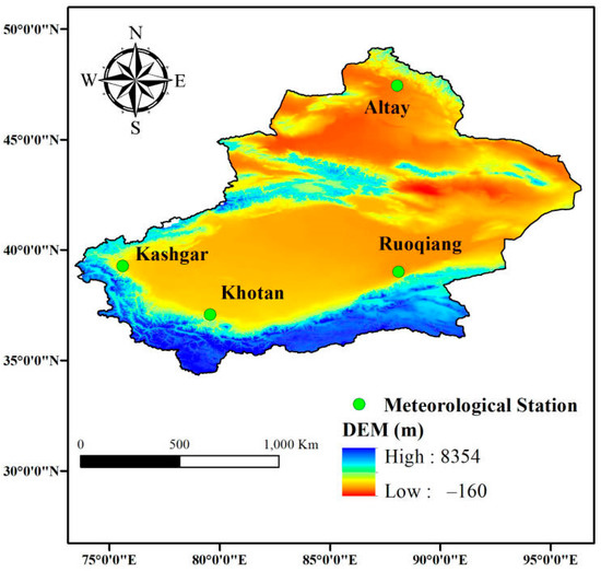
Figure 1.
Location of the meteorological stations.

Table 1.
Global solar radiation in different months of stations in this study.
NCEP implemented its next Global Ensemble Forecasting System (GEFSv12) in summer 2020. This model upgrade, based on a deterministic and ensemble prediction system, is very different from the previous upgrade. In the NCEP operation model, a new dynamic core (FV3) is used for the first time to replace the previous spectral dynamic core [32]. The previous three categories of Zhao–Carr microphysics schemes have also been replaced by the more advanced six categories of GFDL microphysics schemes. From the perspective of the ensemble model, GEFSv12 extends the prediction period to 35 days. To better represent the considerable uncertainty related to this time scale, random physical-disturbance trends and random kinetic-energy-backscattering stochastic schemes replaced the original random general-disturbance-trend stochastic scheme, which is also a significant upgrade of the system [33]. Its spatial resolution is 25 km and its temporal resolution is 3 h. In this study, we used grid data from the mean of the four grid points around the site, including forecasting solar radiation (Rsf), maximum temperature (Tmaxf), minimum temperature (Tminf), relative humidity (RHf) at 2 m height and wind speed (Uf) at 10 m height every 3 h for the next 72 h, and converted the 3 h time-resolution data into daily data. That means that, for 3 h to 24 h (27 h to 48 h and 51 to 72 h), the eight data points were converted to daily scale. Tmaxf and Tminf are the highest and lowest temperature of the eight time scale in one day. RHf and Uf are the mean of the eight-point time scale in one day. Rsf is the sum of the eight-point time scale in a day. The output of the models is the measured Rs corresponding to the GEFS data on the same day.
The data were also divided into two parts, from 2006 to 2010 for the training model, and from 2011 to 2015 for validation.
2.2. Quantile Mapping (QM)
QM algorithms are commonly used to correct forecasting and observed data [34,35]. The QM method assumes that forecast data has the same cumulative frequency distribution (CDF) as observed data. The general equation of the QM method is defined as follows:
where is the model forecast data at the t time. is the CDF of the observed history data. is the inverse of CDF observed historical data.
2.3. Equiratio Cumulative Distribution Function Matching (EDCDFm)
EDCDFm is also a method based on quantile mapping. However, unlike the QM method, EDCDFm believes that observed value and forecast value have different CDFs [36]. The difference in CDF function needs to be considered, which is defined as follows:
where is the CDF of the model forecasting data in the future, and is the inverse of CDF model forecasting historical data.
2.4. Machine-Learning Algorithms
2.4.1. Long-Short Term Memory (LSTM)
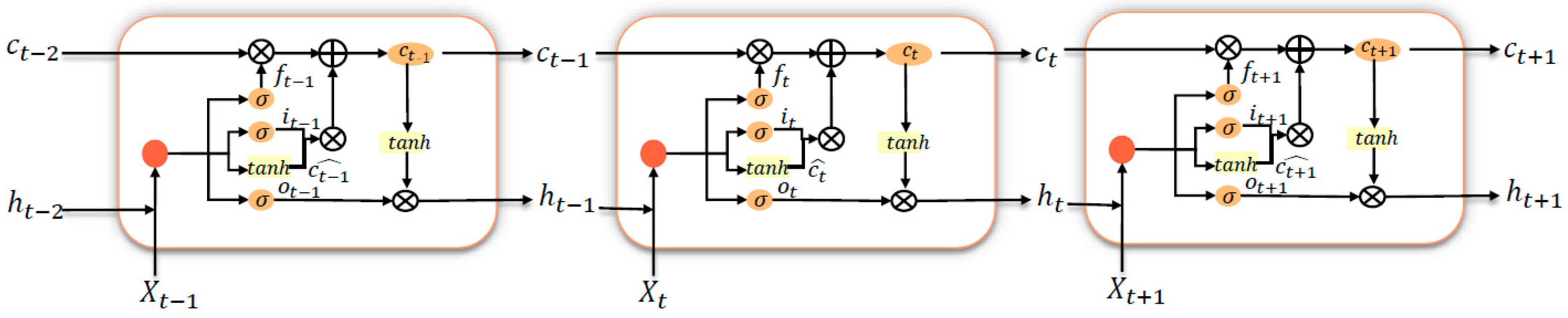
In recent years, due to the advantages of LSTM model in dealing with sequential tasks, researchers have carried out a lot of research on it [37,38,39]. LSTM is a deep-learning architecture that aims to solve the long-term dependence problem of existing recurrent neural networks (RNNs) by introducing forgetting gates. LSTM model can recall previous data and evaluate the correlation of features based on past data.
As shown in Figure 2, a typical LSTM network consists of one unit and three gates (input gate, forget gate and output gate). The input gate adjusts the amount of new data stored in the unit. The output gate determines which information to obtain from the cell, while the forgetting gate determines which information can be discarded. The LSTM model will consider all this information and make judgments. These gates control cell state Ct and output ht; the input gate can be calculated as follows:
where is the sigmoid activation function, is the cell output at the previous time step, and are the weighting factors, and is the bias. The forget gate can be calculating as follows:
where and are the weighting factors, and is the bias. The equation of output gate is as follows:
where and are the weighting factors, and is the bias.
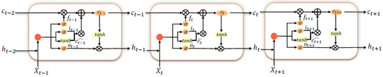
Figure 2.
The struct of the LSTM model.
In this study, LSTM is used to forecast Rs, and the input data includes Rsf, Tmaxf, Tminf, RHf and Uf for the forecast target day and observed Rs values during the previous 3–6 days. To achieve this model, Python 3.7 (https://www.python.org/downloads/release/python-370/ (accessed on 25 April 2022)) was used to develop the model.
2.4.2. Support Vector Machine (SVM)
SVM is an advanced statistical method based on the structural risk minimization principle and Vapnik–Chervonenkis dimension theory [40]. This method can be used to deal with classification and regression problems. Support vector regression (SVR) is an extension of a support vector machine in the field of regression. It has the advantages of solid generalization ability and fast convergence speed. It also has the advantages of dealing with small samples and nonlinear problems. By introducing the structural error minimization criterion, SVR has good robustness, generalization and learning ability. The SVR function is defined as follows:
where is the output, w is the weight vector, is the high-dimensional nonlinear mapping function, and is the constant. This equation is equivalent to the following objective function:
where is the penalty parameter, n is the number of the samples for develop the model, is the maximum allowable error which depending on the samples, and is the residual error, defined as follows:
By introducing two relaxation variables (ζ and ζ* ), Equation (5) can be rewritten as:
Equation (6) can be converted into a duality problem as:
where and are the Lagrange multipliers, and is a kernel function.
There are many kinds of kernel functions. In this study, we used radial basis function as kernel function, which has certain advantages in nonlinear aspect.
2.4.3. Extreme Gradient Boosting (XGBoost)
XGBoost is the first parallel gradient enhanced tree (GBDT) algorithm. XGBoost, based on classification and regression tree (CART) theory, has been widely proven to be a very efficient approach to regression and classification problems [41]. After optimization, XGBoost’s objective function consists of two different parts, representing the deviation and regularization terms of the model to prevent overfitting. The objective function can be written as follows:
where and are parameters that measure model complexity. is the number of leaves on the CART tree, and is also a weight parameter; in XGBoost, this is the weight of each leaf. More details can be found in the reference [41].
2.4.4. Kernel-Based Nonliear Extension of Arps Decline (KNEA)
KNEA is a new time-series model which has been applied in oil-production estimation, ET0 prediction and groundwater-level prediction [42,43]. The KNEA synthesizes nonlinear models of past state and present effects. The main function of KNEA algorithm can be expressed as:
where is the output at present; is the output of the previous step; is the variables that can affect the output; is a function of variables; and a and b are the constants. Usually, the is unknown, so it should be converted to:
where is the nonlinear mapping of variable into a new space.
After transformation, a small value can be introduced in the function and the original problem is transformed into a minima problem:
Similar to SVM, this equivalent form can also be solved by introducing Lagrange multipliers and kernel functions.
2.4.5. Bat Algorithm
Yang and He [44] proposed the bat algorithm by imitating the predation law of bats. Bat algorithm has high efficiency in parameter optimization. Velocity and position changes are critical for bats to find optimal solutions in space, and these values are obtained by the following equation:
where is a random vector and its value range is [−1, 1]; is the current optimal position in all the bats; and and are adjust the coefficient of speed. After each generation, each bat produces a new position, as follows:
where is also a random vector and its value range is [−1, 1]; the following steps implement conditional updates of bat positions. A random number is generated and every bat of this generation is traversed. When the random number is greater than and the fitness of the bat is higher than the optimal fitness of the current population, the generated new solution is accepted, and as well as are updated:
where = 0.99, and = 0.5. Equations (20)–(25) are repeated until the maximum generation is reached. BA has been used to optimize the parameters of the machine-learning models, e.g., SVM, XGBoost and KNEA. In this study, the population of BA algorithm was set to 50 and the number of iterations was 200.
The range of parameters of the three machine-learning models are shown in Table 2.
Table 2.
Parameters of the three machine-learning models.
2.4.6. Particle Swarm Optimization Algorithm (PSO)
PSO is an algorithm developed by simulating group predation to find the optimal solution [45,46]. The particle swarm optimization algorithm designs a massless particle with only two attributes: speed and position, in which speed represents the speed of movement and position represents the direction of movement. Each particle searches for the optimal solution separately in the search space and records it as the current individual extreme value. The position of the extreme value is shared with other particles in the whole particle swarm. After other particles find the optimal individual extreme value, they update it to the whole particle swarm’s current global optimal solution. The formula of position and speed of the PSO algorithm is as follows:
where is the location of the i-th particle during t-th iteration, is the speed of the i-th particle during t-th iteration, c1 and c2 are study factors and the value was set as 2. and are random data ranged [−1, 1]. is the best location of the i-th particle among different iterations. is the globally best location of all the particles. is the momentum factor, which can be calculated as follows:
where and are the initial and the end momentum factors, and the values were set as 0.9 and 0.4, respectively. is the maximum iteration. In this study, the population of PSO algorithm was set to 50 and the number of iterations was 200. The range of machine-learning parameters optimized by PSO is the same as the BA algorithm. Figure 3 presents the flow chart of three machine-learning models optimized by evolutionary algorithms. To achieve these models, except LSTM, R language (R language v4.4, https://www.r-project.org/ (accessed on 25 April 2022)) was used.
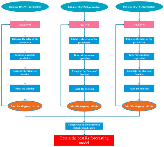
Figure 3.
Flowchart of the three machine-learning models optimal for evolutionary algorithms.
2.5. Statistical Indicators
In this study, four commonly used statistical indicators were used to evaluate the prediction performance of total surface radiation, which are determination coefficient (R2):
Root mean square error (RMSE):
Mean absolute error:
Normalized RMSE:
where Rs,m is measured Rs, Rs,f is forecasting Rs, is the mean of the measured Rs, and is the mean of forecasting Rs.
3. Results
3.1. Empirical Statistics Methods
Table 3 presents the statistical indicators of the GEFSv12 NWP raw Rsf forecasting data and the results from QM and EDCDFm methods. In general, with the extension of the forecast period, the errors of NWP raw Rsf data and the Rsf correct by QM and EDCDFm methods gradually increase. In Altay, the performance of the QM and EDCDFm methods were very similar, and both of them were slightly better than that of the NWP raw Rsf data. In Kashgar, the error of the raw Rsf data was relatively large. However, the QM and EDCDFm methods were superior to the raw Rsf, with RMSE decreased by 28.2–31% and 28.6–31.5%, and MAE decreased by 27.9–31.1% and 27.7–31.1%, respectively, during 1–3 d ahead. In Ruoqiang, the error of the raw Rsf was large, and its RMSE was more than 5 MJ m−2 d−1. After correcting by QM and EDCDFm method correction, RMSE decreased by 17.4–18.5% and 19.7–20.1% for 1–3 d ahead, and MAE decreased by 16–17.7% and 17.7–19.4%, respectively. However, the R2 of the raw Rsf was slightly higher than that of the two statistical methods. This indicates that the statistical method improved the overestimation (or underestimation) problem. The performance for Khotan station was similar to that of Ruoqiang station. Compared with the raw Rsf over the four stations, the RMSE and MAE of QM and EDCDFm models decreased by 20% and 15%, respectively. It can be seen from the above results that empirical statistical methods can improve forecasting accuracy.
Table 3.
Statistical indicators of solar-radiation forecast by GEFS NWP raw data and two empirical-statistics methods.
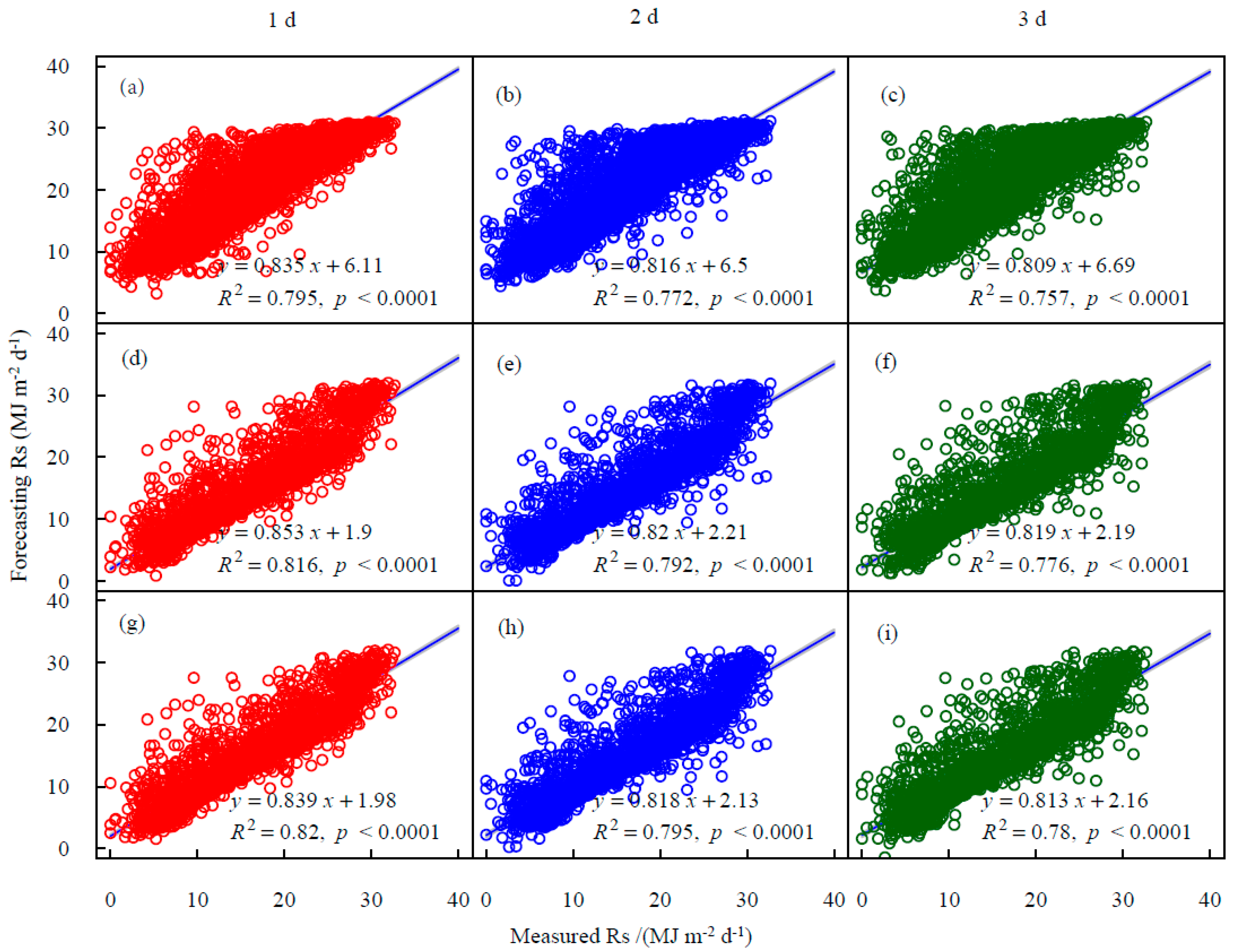
As can be seen from the scatter plot of raw Rs vs. ground observed Rs (Figure 4), the discrete points increased slightly from 1 d to 3 d, indicating a slight decrease in inaccuracy. The forecasting value of Rsf in the future 1–3 d was not higher than 30 MJ m−2 d−1, which was slightly lower than the extreme value of Rs. The main problem of the GEFS data set lay in the existence of many overestimated discrete points when the observed value was lower than 25 MJ m−2 d−1. However, the QM and EDCDFm methods can alleviate this problem, and the R2 of the two methods was slightly higher than the corresponding value of raw Rsf data.
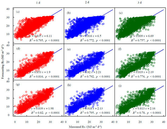
Figure 4.
Scatter plots of measured Rs vs. forecasting Rs at Kashgar station during the testing period, GEFSv12 raw Rs forecasting data on (a) 1 d ahead, (b) 2 d ahead, (c) 3 d ahead; QM method forecasting Rs on (d) 1 d ahead, (e) 2 d ahead, (f) 3 d ahead; EDCDFm method forecasting Rs on (g) 1 d ahead, (h) 2 d ahead, (i) 3 d ahead.
3.2. Machine-Learning Methods
Table 4 shows the statistical indicators of Rs-forecasting results by seven different machine-learning methods during 1–3 d ahead. In Altay, the third day’s R2 average increased by 0.046, and the average RMSE and MAE increased by 13.4% and 13.1%, compared with the first day. Among the seven machine-learning models, the BA-KNEA model was superior to other machine−learning models each day, and the RMSE, MAE and NRMSE of the BA-KNEA model decreased by 2.1–10.3%, 2.5–12.0% and 2.8–12.4% than other machine-learning models for 1 d ahead, decreased by 1.8–8.8%, 1.7% to 10.1% and 1.6–9.9% for 2 d ahead, and decreased by 2.2–8.2%, 2.2–9.6% and 2.0–9.5% for 3 d ahead. The performance of the BA-SVM model was ranked second, followed by BA-XGBoost, PSO-KNEA, PSO-SVM, LSTM and PSO-XGBoost models.
Table 4.
Statistical indicators of solar-radiation forecasts by different machine-learning models.
In Kashgar, the BA-KNEA model did not have a significant advantage over the PSO-KNEA model on the first two days, but performed slightly better than the PSO-KNEA model on the third day. In addition, the BA-KNEA model was generally superior to other models. RMSE, MAE and NRMSE decreased by 3.8–7.0%, 0–6.2% and 0–6.3% for 1 d ahead, 3.8–8.4%, 2.8–8.6% and 2.4–8.2% for 2 d ahead, and 5.4–12.5%, 2.3–14.7% and 2.3–14.5% for 3 d ahead. In addition, the BA-XGBoost model slightly outperformed the BA-SVM model.
In Ruoqiang, the BA-KNEA model performed better than the other six models. Compared with the BA-KNEA model, the RMSE, MAE and NRMSE of the other six models increased by 4.6–9.6%, 4.6–10.6% and 4.5–10.5% for 1 d ahead, 7.1–10.0%, 4.9–9.5%, 6.3–9.7% for 2 d ahead, and 3.3–4.9%, 2.6–4.6%, 3.2–5.1% for 3 d ahead. The BA-SVM model performed better than the other four models on 1 d, but the advantage in the other models, except BA-KNEA, was not obvious on the other two days. In Khotan, the BA-KNEA model also achieved the highest accuracy, and the RMSE, MAE and NRMSE of the other five models increased by 2.6–6.9%, 4.8–7.1% and 1.3–6.7% for 1 d ahead, 3.5–9.0%, 1.6–8.4%, 1.2–8.5% for 2 d ahead, and 3.0–8.5%, 1.8–12.8%, 1.8–11.8% for 3 d ahead. The performance of the BA-SVM model was still better than the other four models, except for the BA-KNEA model.
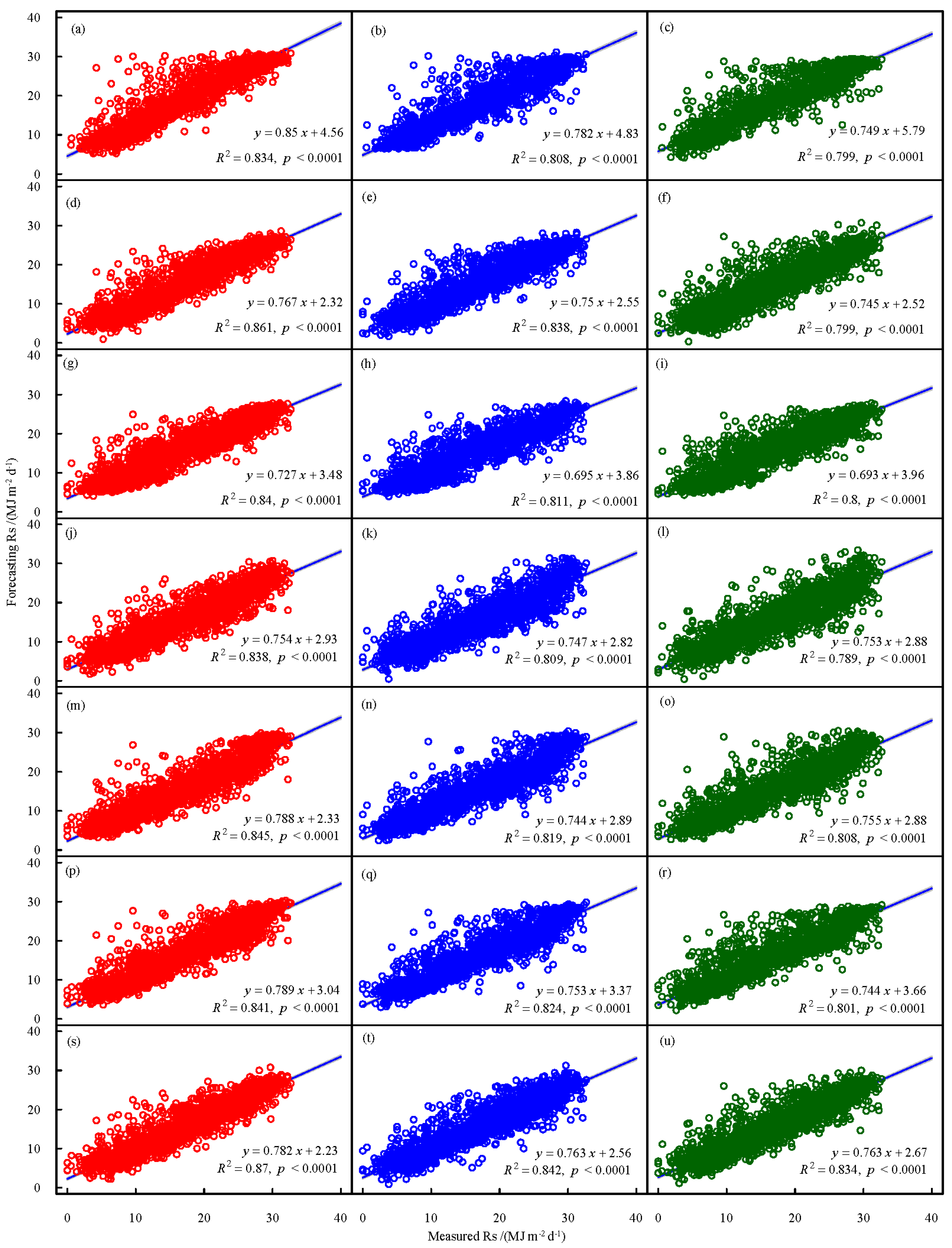
The scatter plots of observed Rs vs. Rsf by seven machine-learning models are shown in Figure 5. Among all the machine-learning models, it can be seen that the BA-KENA model performed slightly better than other models, followed by the BA-SVM model. The slope of all the regression equations in the Figure was less than 1, and the intercept was greater than 0, which means that all the models exhibit the problem that when Rs is very large, the model will underestimate the result, and when Rs is very small, the model will underestimate the result.
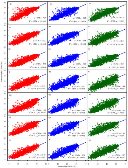
Figure 5.
Scatter plots of measured Rs vs. forecasting Rs at Kashgar station during the testing period, LSTM method forecasting data on (a) 1 d ahead, (b) 2 d ahead, (c) 3 d ahead; PSO-SVM method forecasting Rs on (d) 1 d ahead, (e) 2 d ahead, (f) 3 d ahead; BA-SVM method forecasting Rs on (g) 1 d ahead, (h) 2 d ahead, (i) 3 d ahead; PSO-XGBoost method forecasting Rs on (j) 1 d ahead, (k) 2 d ahead, (l) 3 d ahead; BA-XGBoost method forecasting Rs on (m) 1 d ahead, (n) 2 d ahead, (o) 3 d ahead; PSO-KNEA method forecasting Rs on (p) 1 d ahead, (q) 2 d ahead, (r) 3 d ahead; BA-KNEA method forecasting Rs on (s) 1 d ahead, (t) 2 d ahead, (u) 3 d ahead.
Figure 6 shows the distribution of the absolute error of the forecast Rs for different machine-learning models 1–3 days ahead. As can be seen, at 1 d ahead, the proportion of days with AE < 2 MJ m−2 d−1 for the six models was around 60%; the proportion of PSO-KNEA and BA-KNEA was slightly higher than in other models; and had a AE > 6 MJ m−2 d−1 days ratio, the BA-KNEA had a slight advantage over the other models. The performance on 2 d ahead was slightly worse than that on 1 d ahead: the proportion of days with AE < 2 MJ m−2 d−1 for all six models was below 60%, while the number of days with AE > 6 MJ m−2 d−1 showed little change compared with 1 d ahead, with the BA-KNEA model having a slight advantage over the other models in the number of days with AE > 6 MJ m−2 d−1. In the 3 d ahead, the accuracy of the six models continued to decline compared with the previous 2 d, and the BA-KNEA model had a slightly lower proportion of days with AE > 6 MJ m−2 d−1 than the other models.
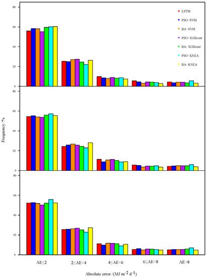
Figure 6.
Absolute error of different machine−learning models at Ruoqiang station.
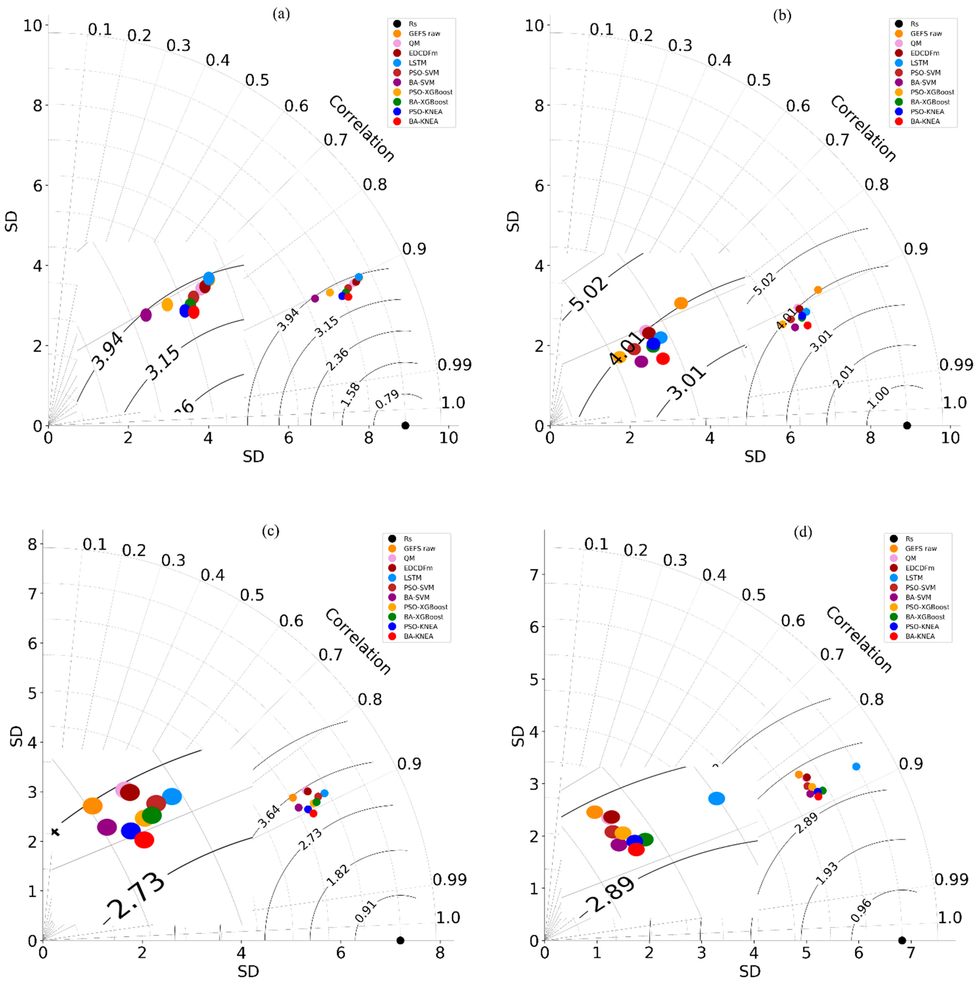
Figure 7 shows the Taylor diagram of different methods over the four stations. It can be seen that the BA-KNEA model outperformed the other methods over the all stations.
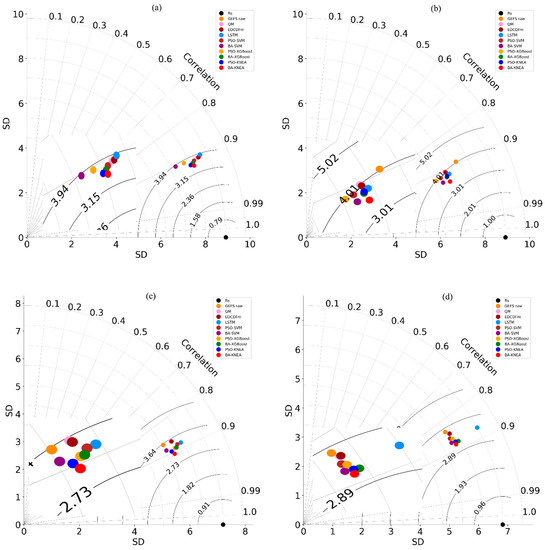
Figure 7.
Taylor plots of forecasting results for different Rs.
3.3. Comparison of Statistical Models and Machine-learning Models
To evaluate the performance of different categories of models, we ranked the four statistical indicators of all models over the four stations (Table 5). With the highest R2 or the lowest RMSE, MAE or NRMSE would rank first, and so on. When the ranking of different statistical indicators is different, the model with more indicators at the top ranks first. It can be seen that the rank of different models in 1–3 d ahead were the same. The BA-KNEA model was the best, followed by the BA-SVM, BA-XGBoost, PSO-KNEA, PSO-SVM, LSTM, PSO-XGBoost, EDCDFm and QM models. The above results prove that the machine−learning model is superior to the empirical-statistical model, and the new BA-KNEA model has the best performance in accuracy. In addition, the Taylor plots of different stations on the first day of the forecast period are shown in Figure 6. It can also be seen that the results of the BA-KNEA model were the closest to the observations, while the GEFS raw data had the largest error.
Table 5.
Rank of empirical-statistical and machine-learning models.
3.4. BA-KNEA with Different Input Combinations
In order to analyze the difference in the forecasting ability of different meteorological factors on the results, we used the BA-KNEA model to set up different input combinations. Through the results, we explored the contribution differences of different factors. Table 6 shows the statistical indicators of the different input combinations of the BA-KNEA model in the forecast period 1–3 d. When the input factor is Rsf, the accuracy of the BA-KNEA model was better than that of the QM and EDCDFm methods with the same input at four stations (Table 3), and the RMSE and MAE of the BA-KNEA model was 1.7–7.9% and was 1.6–7.6% lower in the forecast period of 1–3 days, relative to the EDCDFm method. This model was also better than the model established with temperature and extraterrestrial radiation as inputs (Combination 5), which shows that the solar radiation accuracy of the GEFSv12 dataset is better than that of the traditional temperature-based machine-learning model method. In Altay, when only the maximum and minimum air temperature was used as input, the error was larger than the model with Rs input: R2 was between 0.712–0.723, RMSE was between 4.705–4.812 MJ m−2 d−1, and MAE was between 3.766–3.799 MJ m−2 d−1, and NRMSE was between 0.241–0.243. Adding RHf, Uf, Tmaxf and Tminf based on the Rsf can improve the prediction accuracy of Rs, among which the increase in wind speed was the largest, followed by air temperature, and, finally, relative humidity. Compared with Combination 2, 3, and 4, the accuracy of combination 6 was higher, and it can be seen that the accuracy of the multi-factor was higher than that of the two-factor combination. This shows that the multi-factor combination contains more nonlinear information related to Rs than the two-factor combination, which helps improve the model accuracy further. At Kashgar station, adding relative humidity based on Rs did not improve the accuracy significantly, and when the forecast period was 2 and 3 days, adding wind speed based on Rs slightly improved the accuracy. Adding the temperature model based on Rs improves the model’s accuracy to a certain extent, but it is not much different from the accuracy of the complete combination (Combination 6). This is mainly due to the limited contribution of RH and U to improving the accuracy of the model. The performance of the BA-KNEA model on the first two days of Ruoqiang Station was similar to that on Altay, but on the third day, Combination 3 outperformed the complete input combination. Due to poor forecast accuracy of wind speed and relative humidity, adding these factors will increase the noise in the model. At Khotan station, on the first day, the complete combination was close to the Combination 2, 3, and 4 but superior to those during the other two days. The complete combination is slightly better than the other combinations. As seen from the above, the complete combination was slightly better than the other combinations over the four stations.
Table 6.
Statistical indicators of BA-KNEA model under different input combinations.
4. Discussion
Different machine-learning models perform differently in solar-radiation prediction. This is mainly due to two reasons. Firstly, different machine-learning models have different sensitivities to data distribution. For example, kernel-based machine-learning methods can perform well in low-dimensional data sets [47]. However, the tree-based model performs better with high dimensions and a large amount of typed data. The deep-learning model has better performance in image processing [48]. Another reason is that the parameter selection of machine-learning models did not achieve the optimal global solution. Fan et al. [31] compared the performance of SVM and XGBoost when the input factors were temperature and precipitation and found that SVM was slightly better than the XGBoost model. Ghimire et al. [7] compared ANN, SVR, GPML and GP models for forecasting solar radiation with reanalysis data in Queensland, Australia. They highlighted that the ANN model outperformed other ML models. Shin et al. [49] used a deep-learning model to short-term forecast solar radiation for photovoltaic power generation. Hu et al. [50] used ground-based images and an ANN model to forecast solar radiation. However, there is limited study of using weather-forecast products to forecast solar radiation in China. In this study, we evaluated the capability of the GEFSv12 product in the solar-resource-rich region of China. We found that the raw solar-radiation forecast data in GEFSv12 has poor performance and uncertainty for indirect use. Thus, we built a coupling model based on the bat algorithm and KNEA model. The result shows that the newly developed model is superior to other empirical-statistical and machine-learning models. The LSTM had been used to forecast Rs on hourly and other time scales [51,52]. However, we found that the LSTM did not perform better than the BA-KNEA model nor other models. The daily Rs fluctuated widely on an hourly scale in the arid regions of the northwest of China, and historical information is not as important as the WRF data for future. Thus, the LSTM did not achieve enough information to forecast 1–3 d Rs.
Many scholars have found that various meteorological factors, such as air temperature, relative humidity, wind speed, and precipitation, are closely related to solar radiation [53,54], but the effects of these factors vary in different regions of the globe [55,56]. In northwest China, air temperature is the closest meteorological variable to solar radiation [57]. Thus, many scholars have established solar-radiation models based on air temperature. In addition, relative humidity and wind speed have also been used to improve the accuracy of solar radiation prediction [58,59]. Although the forecast data set was used in this study, similar results have been obtained, which means that the forecast data set and observation data have similar results. The most significant difference between the forecast data set and observation data lies in the forecast precision of different forecast factors. In general, the temperature has a very high forecast accuracy, but the relative humidity and wind-speed forecast accuracy are low, a fact mainly caused by two data mismatches. That is to say, the forecast data is the average of a large area, while the relative humidity and wind speed observed by the weather station is a minimal point value. We found that, in the four stations of this study, the model’s accuracy with temperature factor is generally better than that of wind speed and relative humidity, and the prediction performance of relative humidity and wind speed of GEFSv12 needs to be improved.
5. Conclusions
Accurate forecasting of solar radiation (Rs) is significant to photovoltaic power generation and agricultural management. For the first time, this study evaluated and improved the capability of the newly released National Centers for Environmental Prediction Global Ensemble Forecast System version 12 (NECP GEFSv12) for short-term forecasting of Rs. To achieve this goal, a new coupling model based on the bat algorithm (BA) and kernel-based nonlinear extension of Arps decline (KNEA) was established. The data used four solar-radiation stations in Xinjiang, China as the benchmark. The new model was also compared with two empirical statistical methods (quantile mapping and Equiratio cumulative distribution function matching) with five machine-learning methods, e.g., support vector machine (SVM), XGBoost, KNEA, BA-SVM, BA-XGBoost. The results show that the accuracy of forecasting Rs from all of the models decreases from 1 d to 3 d ahead. Compared with the GEFS raw Rs data over the four stations, the RMSE and MAE of the QM and EDCDFm models decreased by 20% and 15%, respectively. In addition, the BA-KNEA model was superior to the GEFSv12 raw Rs data and other post-processing methods, with R2 = 0.782–0.829, RMSE= 3.240–3.685 MJ m−2 d−1, MAE = 2.465–2.799 MJ m−2 d−1, NRMSE = 0.152–0.173.
Author Contributions
Conceptualization, L.W.; methodology, L.W. and F.L.; software, S.W.; validation, G.D.; formal analysis, G.D.; investigation, G.D.; resources, data curation, S.W.; writing—original draft preparation, L.W. and G.D.; writing—review and editing, G.D. and L.W.; supervision, F.L.; project administration, Y.W.; funding acquisition, S.W. All authors have read and agreed to the published version of the manuscript.
Funding
This study was jointly supported by the National Natural Science Foundation of China (No. 51879226, 51709143) and Jiangxi Natural Science Foundation of China (No. 20181BBG78078). The APC was funded by Jiangxi Natural Science Foundation of China (No. 20181BBG78078).
Institutional Review Board Statement
Not applicable.
Informed Consent Statement
Not applicable.
Data Availability Statement
Not applicable.
Acknowledgments
Thanks to the National Meteorological Information Center of China Meteorological Administration for offering the meteorological data.
Conflicts of Interest
The authors declare no conflict of interest.
References
- Liu, P.; Tong, X.; Zhang, J.; Meng, P.; Li, J.; Zheng, J. Estimation of half-hourly diffuse solar radiation over a mixed plantation in north China. Renew. Energy 2020, 149, 1360–1369. [Google Scholar] [CrossRef]
- Demircan, C.; Bayrakçı, H.C.; Keçebaş, A. Machine learning-based improvement of empiric models for an accurate estimating process of global solar radiation. Sustain. Energy Technol. Assess. 2020, 37, 100574. [Google Scholar] [CrossRef]
- Chang, K.; Zhang, Q. Improvement of the hourly global solar model and solar radiation for air-conditioning design in China. Renew. Energy 2019, 138, 1232–1238. [Google Scholar] [CrossRef]
- Zang, H.; Cheng, L.; Ding, T.; Cheung, K.W.; Wang, M.; Wei, Z.; Sun, G. Application of functional deep belief network for estimating daily global solar radiation: A case study in China. Energy 2019, 191, 116502. [Google Scholar] [CrossRef]
- Rehman, S.; Mohandes, M. Artificial neural network estimation of global solar radiation using air temperature and relative humidity. Energy Policy 2008, 36, 571–576. [Google Scholar] [CrossRef] [Green Version]
- Quej, V.H.; Almorox, J.; Arnaldo, J.A.; Saito, L. ANFIS, SVM and ANN soft-computing techniques to estimate daily global solar radiation in a warm sub-humid environment. J. Atmos. Sol.-Terr. Phys. 2017, 155, 62–70. [Google Scholar] [CrossRef] [Green Version]
- Ghimire, S.; Deo, R.C.; Raj, N.; Mi, J. Deep solar radiation forecasting with convolutional neural network and long short-term memory network algorithms. Appl. Energy 2019, 253, 113541. [Google Scholar] [CrossRef]
- Deo, R.C.; Şahin, M.; Adamowski, J.F.; Mi, J. Universally deployable extreme learning machines integrated with remotely sensed MODIS satellite predictors over Australia to forecast global solar radiation: A new approach. Renew. Sustain. Energy Rev. 2019, 104, 235–261. [Google Scholar] [CrossRef]
- Hassan, M.A.; Khalil, A.; Kaseb, S.; Kassem, M.A. Exploring the potential of tree-based ensemble methods in solar radiation modeling. Appl. Energy 2017, 203, 897–916. [Google Scholar] [CrossRef]
- Güçlü, Y.S.; Yeleğen, M.Ö.; Dabanlı, İ.; Şişman, E. Solar irradiation estimations and comparisons by ANFIS, Angström–Prescott and dependency models. Sol. Energy 2014, 109, 118–124. [Google Scholar] [CrossRef]
- Mohammadi, K.; Shamshirband, S.; Kamsin, A.; Lai, P.C.; Mansor, Z. Identifying the most significant input parameters for predicting global solar radiation using an ANFIS selection procedure. Renew. Sustain. Energy Rev. 2016, 63, 423–434. [Google Scholar] [CrossRef]
- Feng, Y.; Cui, N.; Chen, Y.; Gong, D.; Hu, X. Development of data-driven models for prediction of daily global horizontal irradiance in northwest China. J. Clean. Prod. 2019, 223, 136–146. [Google Scholar] [CrossRef]
- Wu, L.; Huang, G.; Fan, J.; Zhang, F.; Wang, X.; Zeng, W. Potential of kernel-based nonlinear extension of Arps decline model and gradient boosting with categorical features support for predicting daily global solar radiation in humid regions. Energy Convers. Manag. 2019, 183, 280–295. [Google Scholar] [CrossRef]
- Fan, J.; Wu, L.; Zhang, F.; Cai, H.; Wang, X.; Lu, X.; Xiang, Y. Evaluating the effect of air pollution on global and diffuse solar radiation prediction using support vector machine modeling based on sunshine duration and air temperature. Renew. Sustain. Energy Rev. 2018, 94, 732–747. [Google Scholar] [CrossRef]
- Fan, J.; Wu, L.; Ma, X.; Zhou, H.; Zhang, F. Hybrid support vector machines with heuristic algorithms for prediction of daily diffuse solar radiation in air-polluted regions. Renew. Energy 2020, 145, 2034–2045. [Google Scholar] [CrossRef]
- Belaid, S.; Mellit, A. Prediction of daily and mean monthly global solar radiation using support vector machine in an arid climate. Energy Convers. Manag. 2016, 118, 105–118. [Google Scholar] [CrossRef]
- Urraca, R.; Martinez-de-Pison, E.; Sanz-Garcia, A.; Antonanzas, J.; Antonanzas-Torres, F. Estimation methods for global solar radiation: Case study evaluation of five different approaches in central Spain. Renew. Sustain. Energy Rev. 2017, 77, 1098–1113. [Google Scholar] [CrossRef]
- Álvarez-Alvarado, J.M.; Ríos-Moreno, J.G.; Obregón-Biosca, S.A.; Ronquillo-Lomelí, G.; Ventura-Ramos, E.; Trejo-Perea, M. Hybrid techniques to predict solar radiation using support vector machine and search optimization algorithms: A review. Appl. Sci. 2021, 11, 1044. [Google Scholar] [CrossRef]
- Dong, J.; Wu, L.; Liu, X.; Fan, C.; Leng, M.; Yang, Q. Simulation of daily diffuse solar radiation based on three machine learning models. Comput. Model. Eng. Sci. 2020, 123, 49–73. [Google Scholar] [CrossRef]
- Feng, Y.; Hao, W.; Li, H.; Cui, N.; Gong, D.; Gao, L. Machine learning models to quantify and map daily global solar radiation and photovoltaic power. Renew. Sustain. Energy Rev. 2020, 118, 109393. [Google Scholar] [CrossRef]
- Liu, Y.; Zhou, Y.; Chen, Y.; Wang, D.; Wang, Y.; Zhu, Y. Comparison of support vector machine and copula-based nonlinear quantile regression for estimating the daily diffuse solar radiation: A case study in China. Renew. Energy 2020, 146, 1101–1112. [Google Scholar] [CrossRef]
- Qing, X.; Niu, Y. Hourly day-ahead solar irradiance prediction using weather forecasts by LSTM. Energy 2018, 148, 461–468. [Google Scholar] [CrossRef]
- Abdel-Nasser, M.; Mahmoud, K. Accurate photovoltaic power forecasting models using deep LSTM-RNN. Neural Comput. Appl. 2019, 31, 2727–2740. [Google Scholar] [CrossRef]
- Huang, C.; Kuo, P. Multiple-input deep convolutional neural network model for short-term photovoltaic power forecasting. IEEE Access 2019, 7, 74822–74834. [Google Scholar] [CrossRef]
- Kaba, K.; Sarıgül, M.; Avcı, M.; Kandırmaz, H.M. Estimation of daily global solar radiation using deep learning model. Energy 2018, 162, 126–135. [Google Scholar] [CrossRef]
- Voyant, C.; Notton, G.; Kalogirou, S.; Nivet, M.; Paoli, C.; Motte, L.; Fouilloy, A. Machine learning methods for solar radiation forecasting: A review. Renew. Energy 2017, 105, 569–582. [Google Scholar] [CrossRef]
- Sun, H.; Gui, D.; Yan, B.; Liu, Y.; Liao, W.; Zhu, Y.; Lu, C.; Zhao, N. Assessing the potential of random forest method for estimating solar radiation using air pollution index. Energy Convers. Manag. 2016, 119, 121–129. [Google Scholar] [CrossRef] [Green Version]
- Ibrahim, I.A.; Khatib, T. A novel hybrid model for hourly global solar radiation prediction using random forests technique and firefly algorithm. Energy Convers. Manag. 2017, 138, 413–425. [Google Scholar] [CrossRef]
- Prasad, R.; Ali, M.; Kwan, P.; Khan, H. Designing a multi-stage multivariate empirical mode decomposition coupled with ant colony optimization and random forest model to forecast monthly solar radiation. Appl. Energy 2019, 236, 778–792. [Google Scholar] [CrossRef]
- Hamill, T.M.; Whitaker, J.S.; Shlyaeva, A.; Bates, G.; Fredrick, S.; Pegion, P.; Sinsky, E.; Zhu, Y.; Tallapragada, V.; Guan, H.; et al. The Reanalysis for the Global Ensemble Forecast System, Version 12. Monthly. Weather Rev. 2022, 150, 59–79. [Google Scholar] [CrossRef]
- Fan, J.; Chen, B.; Wu, L.; Zhang, F.; Lu, X.; Xiang, Y. Evaluation and development of temperature-based empirical models for estimating daily global solar radiation in humid regions. Energy 2018, 144, 903–914. [Google Scholar] [CrossRef]
- Zhou, X.; Zhu, Y.; Hou, D.; Fu, B.; Li, W.; Guan, H.; Sinsky, E.; Kolczynski, W.; Xue, X.; Luo, Y.; et al. The Development of the NCEP Global Ensemble Forecast System Version 12. Weather Forecast. 2022, 37, 727. [Google Scholar] [CrossRef]
- Tallapragada, V. Recent updates to NCEP Global Modeling Systems: Implementation of FV3 based Global Forecast System (GFS v15. 1) and plans for implementation of Global Ensemble Forecast System (GEFSv12). In AGU Fall Meeting Abstracts; Astrophysics Data System: San Francisco, CA, USA, 2019; pp. A31C–A34C. [Google Scholar]
- Lee, T.; Singh, V.P. Statistical Downscaling for Hydrological and Environmental Applications; CRC Press: Boca Raton, FL, USA, 2018. [Google Scholar] [CrossRef]
- Maraun, D. Bias correction, quantile mapping, and downscaling: Revisiting the inflation issue. J. Clim. 2013, 26, 2137–2143. [Google Scholar] [CrossRef] [Green Version]
- Guo, L.; Gao, Q.; Jiang, Z.; Li, L. Bias correction and projection of surface air temperature in LMDZ multiple simulation over central and eastern China. Adv. Clim. Chang. Res. 2018, 9, 81–92. [Google Scholar] [CrossRef]
- Yu, Y.; Si, X.; Hu, C.; Zhang, J. A review of recurrent neural networks: LSTM cells and network architectures. Neural Comput. 2019, 31, 1235–1270. [Google Scholar] [CrossRef]
- Yan, R.; Liao, J.; Yang, J.; Sun, W.; Nong, M.; Li, F. Multi-hour and multi-site air quality index forecasting in Beijing using CNN, LSTM, CNN-LSTM, and spatiotemporal clustering. Expert Syst. Appl. 2021, 169, 114513. [Google Scholar] [CrossRef]
- Ao, C.; Zeng, W.; Wu, L.; Qian, L.; Srivastava, A.K.; Gaiser, T. Time-delayed machine learning models for estimating groundwater depth in the Hetao Irrigation District, China. Agric. Water Manag. 2021, 255, 107032. [Google Scholar] [CrossRef]
- Vapnik, V.N. An overview of statistical learning theory. IEEE Trans. Neural Netw. 1999, 10, 988–999. [Google Scholar] [CrossRef] [Green Version]
- Chen, T.; He, T.; Benesty, M.; Khotilovich, V.; Tang, Y.; Benesty, M.; Khotilovich, V.; Tang, Y.; Cho, H.; Chen, K. Xgboost: Extreme Gradient Boosting; R Package Vers. 0.4-2; Xgboost: Seattle, WA, USA, 2015; pp. 1–4. [Google Scholar]
- Ma, X.; Liu, Z. Predicting the oil production using the novel multivariate nonlinear model based on Arps decline model and kernel method. Neural Comput. Appl. 2018, 29, 579–591. [Google Scholar] [CrossRef]
- Lu, H.; Ma, X.; Huang, K.; Azimi, M. Prediction of offshore wind farm power using a novel two-stage model combining kernel-based nonlinear extension of the Arps decline model with a multi-objective grey wolf optimizer. Renew. Sustain. Energy Rev. 2020, 127, 109856. [Google Scholar] [CrossRef]
- Yang, X.; He, X. Bat algorithm: Literature review and applications. Int. J. Bio-Inspired Comput. 2013, 5, 141–149. [Google Scholar] [CrossRef] [Green Version]
- Cui, Y.; Jia, L.; Fan, W. Estimation of actual evapotranspiration and its components in an irrigated area by integrating the Shuttleworth-Wallace and surface temperature-vegetation index schemes using the particle swarm optimization algorithm. Agric. For. Meteorol. 2021, 307, 108488. [Google Scholar] [CrossRef]
- Wang, D.; Tan, D.; Liu, L. Particle swarm optimization algorithm: An overview. Soft Comput. 2018, 22, 387–408. [Google Scholar] [CrossRef]
- Erfani, S.M.; Rajasegarar, S.; Karunasekera, S.; Leckie, C. High-dimensional and large-scale anomaly detection using a linear one-class SVM with deep learning. Pattern Recognit. 2016, 58, 121–134. [Google Scholar] [CrossRef]
- Zang, H.; Liu, L.; Sun, L.; Cheng, L.; Wei, Z.; Sun, G. Short-term global horizontal irradiance forecasting based on a hybrid CNN-LSTM model with spatiotemporal correlations. Renew. Energy 2020, 160, 26–41. [Google Scholar] [CrossRef]
- Shin, D.; Ha, E.; Kim, T.; Kim, C. Short-term photovoltaic power generation predicting by input/output structure of weather forecast using deep learning. Soft Comput. 2021, 25, 771–783. [Google Scholar] [CrossRef]
- Hu, M.; Zhao, B.; Ao, X.; Cao, J.; Wang, Q.; Riffat, S.; Su, Y.; Pei, G. Applications of radiative sky cooling in solar energy systems: Progress, challenges, and prospects. Renew. Sustain. Energy Rev. 2022, 160, 112304. [Google Scholar] [CrossRef]
- Feng, Y.; Zhang, X.; Jia, Y.; Cui, N.; Hao, W.; Li, H.; Gong, D. High-resolution assessment of solar radiation and energy potential in China. Energy Convers. Manag. 2021, 240, 114265. [Google Scholar] [CrossRef]
- De Araujo, J.M.S. Performance comparison of solar radiation forecasting between WRF and LSTM in Gifu, Japan. Environ. Res. Commun. 2020, 2, 045002. [Google Scholar] [CrossRef]
- Zhou, Y.; Liu, Y.; Wang, D.; Liu, X.; Wang, Y. A review on global solar radiation prediction with machine learning models in a comprehensive perspective. Energy Convers. Manag. 2021, 235, 113960. [Google Scholar] [CrossRef]
- Qiu, R.; Li, L.; Wu, L.; Agathokleous, E.; Liu, C.; Zhang, B.; Luo, Y.; Sun, S. Modeling daily global solar radiation using only temperature data: Past, development, and future. Renew. Sustain. Energy Rev. 2022, 163, 112511. [Google Scholar] [CrossRef]
- Makade, R.G.; Chakrabarti, S.; Jamil, B. Development of global solar radiation models: A comprehensive review and statistical analysis for Indian regions. J. Clean. Prod. 2021, 293, 126208. [Google Scholar] [CrossRef]
- Tao, H.; Ewees, A.A.; Al-Sulttani, A.O.; Beyaztas, U.; Hameed, M.M.; Salih, S.Q.; Armanuos, A.M.; Al-Ansari, N.; Voyant, C.; Shahid, S.; et al. Global solar radiation prediction over North Dakota using air temperature: Development of novel hybrid intelligence model. Energy Rep. 2021, 7, 136–157. [Google Scholar] [CrossRef]
- Zhang, Y.; Cui, N.; Feng, Y.; Gong, D.; Hu, X. Comparison of BP, PSO-BP and statistical models for predicting daily global solar radiation in arid Northwest China. Comput. Electron. Agric. 2019, 164, 104905. [Google Scholar] [CrossRef]
- Yadav, A.K.; Chandel, S.S. Solar radiation prediction using Artificial Neural Network techniques: A review. Renew. Sustain. Energy Rev. 2014, 33, 772–781. [Google Scholar] [CrossRef]
- Fan, J.; Wang, X.; Wu, L.; Zhang, F.; Bai, H.; Lu, X.; Xiang, Y. New combined models for estimating daily global solar radiation based on sunshine duration in humid regions: A case study in South China. Energy Convers. Manag. 2018, 156, 618–625. [Google Scholar] [CrossRef]


Publisher’s Note: MDPI stays neutral with regard to jurisdictional claims in published maps and institutional affiliations. |
© 2022 by the authors. Licensee MDPI, Basel, Switzerland. This article is an open access article distributed under the terms and conditions of the Creative Commons Attribution (CC BY) license (https://creativecommons.org/licenses/by/4.0/).