Regional Differences, Distribution Dynamics, and Convergence of Air Quality in Urban Agglomerations in China

Abstract

The urban agglomeration (UA), with a high concentration of population and economy, represents an area with grievous air pollution. It is vital to examine the regional differences, distribution dynamics, and air quality convergence in UAs for sustainable development. In this study, we measured the air quality of ten UAs in China through the Air Quality Index (AQI). We analyzed regional differences, distribution dynamics, and convergence using Dagum’s decomposition of the Gini coefficient, kernel density estimation, and the convergence model. We found that: the AQI of China’s UAs shows a downward trend, and the index is higher in northern UAs than in southern UAs; the differences in air quality within UAs are not significant, but there is a gap between them; the overall difference in air quality tends to decrease, and regional differences in air quality are the primary contributor to the overall difference; the overall distribution and the distribution of each UA move rightward; the distribution pattern, ductility, and polarization characteristics are different, indicating that the air quality has improved and is differentiated between UAs; except for the Guanzhong Plain, the overall UA and each UA have obvious σ convergence characteristics, and each UA presents prominent absolute β convergence, conditional β convergence, and club convergence.

1. Introduction

The average annual growth rate of China’s GDP was as high as 14.3% from 1978 to 2021 [1]. However, with this rapid economic growth [2], the coal-dominated energy structure and extensive economic development have led to excessive consumption of resources and aggravated environmental and ecological damage [3,4]. Air pollution, one of the most prominent environmental problems at present [5], has exerted a series of negative impacts on human health [6], social harmony and stability [7], and sustainable economic growth [8]. In response to this problem, the Chinese government has enacted a series of laws and regulations to oversee the conduct of all walks of life, protect and improve the atmospheric environment, and advance the construction of an ecological culture. At the same time, extensive academic efforts have been made to figure out how to improve air quality.

Research on air quality has been conducted with regard to two aspects: the spatiotemporal distribution and the influencing factors of air quality. Firstly, relevant studies reveal obvious regional differences in air quality [9,10,11,12]. China’s air quality index (AQI) shows a spatial distribution pattern of “high in the north and low in the south” [13]. Urban air pollution is “severe in the east and minor in the west, severe in the north and minor in the south” [14]. In other words, the air pollution is severe in the east of the Heihe-Tengchong Line and the north of the Yangtze River and minor in the south of the Yangtze River and west of the Heihe-Tengchong Line [15]. Regional differences in air quality have also been confirmed in Catalonia in Spain, Detroit, and northern South America [16,17,18]. Air quality also has obvious temporal differences. Specifically, China’s air pollution is high in autumn and winter and low in spring and summer [19,20,21], and there is a U-shaped trend in the monthly average concentration, while the concentration of pollutants in South Africa peaks between June and August [22]. There are also differences in the degree of air pollution in the two different time periods under normal and dusty weather [23]. Secondly, scholars have explored the impact of socioeconomic factors and natural conditions on air quality. The socioeconomic factors influencing air quality include population [24,25], the economy [26,27,28,29], energy consumption [30,31,32], environmental policy [33], income inequality [34], land use [35,36], transportation infrastructure [37,38], etc., with even the large-scale sale of industrial land [39], increase in urbanization rate [40], and foreign direct investment [41] also increasing air pollution. Among the natural factors, meteorological elements such as temperature, precipitation, relative humidity, maximum wind speed, air pressure, and sunshine hours have an important association with air quality [42,43,44,45], and geographical environment elements such as topography [46,47], climate [48,49], and vegetation [50,51,52,53,54] also have an important impact on air quality. In some studies [13,14,15], cluster analysis, geographical concentration index, and spatial autocorrelation analysis are used to measure regional differences in air quality.

The above research results are productive, but little attention has been paid to regional differences in air quality from the perspective of distribution dynamics, and research on the convergence of air quality is extremely scant. Moreover, the urban agglomeration (UA), as the hardest-hit area of air pollution, warrants more attention. Therefore, in the present study, we measured the air quality of ten UAs in China through the AQI and analyzed regional differences, distribution dynamics, and convergence using Dagum’s decomposition of the Gini coefficient, kernel density estimation (KDE), and the convergence model. These methods allow us to discover the sources of regional differences in air quality in UAs and analyze the distribution and convergence of air quality dynamically.

Compared with the existing literature, the contribution of this paper is as follows: firstly, the AQI can objectively and precisely reflect the air quality of UAs, which provides a theoretical basis for air pollution control in UAs; secondly, the regional differences and distribution dynamics of air quality in UAs enrich the research in this field; thirdly, the convergence of air quality in UAs is helpful in revealing the development trend of air quality gaps in UAs.

This paper is organized as follows. The next section of this paper describes the methods and data, including Dagum’s decomposition of the Gini coefficient, KDE, the convergence model, and the data source. The following section presents the findings, including the AQI of UAs, regional differences and their decomposition, distribution dynamics, and convergence. The last section elaborates on the conclusions of this paper and proposes policy implications.

2. Methods and Data

2.1. Methods

2.1.1. Dagum’s Decomposition of the Gini Coefficient

Dagum’s decomposition of the Gini coefficient [55] was used to discuss the regional differences in air quality in various UAs in China, which was calculated as follows:

$$G=\frac{{{\displaystyle \sum }}_{j=1}^k{{\displaystyle \sum }}_{h=1}^k{{\displaystyle \sum }}_{i=1}^{n_j}{{\displaystyle \sum }}_{r=1}^{n_h}\left|y_{ji}-y_{hr}\right|}{2\mu n^2}$$

(1)

where $k$ represents the total number of UAs under investigation; $j$ and $h$ are the subscripts of UAs; $n$ stands for the number of cities under investigation; $i$ and $r$ refer to the subscripts of the cities; $n_j\left(n_h\right)$ is the number of cities in the $j\left(h\right)$th UA; $y_{ji}\left(y_{hr}\right)$ represents the AQI of city $i\left(r\right)$ in the $j\left(h\right)$th UA; and $\mu$ denotes the mean value of the AQI of all cities under investigation. Dagum’s decomposition of the Gini coefficient can be decomposed into intra-UA difference contribution $\left(G_w\right)$, inter-UA net difference contribution $\left(G_{nb}\right)$, and inter-UA intensity of transvariation $\left(G_t\right)$. The specific calculations were based on Equations (2), (4), and (5).

$$G_w={\displaystyle \sum }_{j=1}^k{G}_{jj}{p}_j{s}_j$$

(2)

$$G_{jj}=\frac{1}{2\overline{y_i}}{\displaystyle \sum }_{i=1}^{c_j}{\displaystyle \sum }_{r=1}^{c_j}\left|y_{ji}-y_{jr}\right|/c_j^2$$

(3)

$$G_{nb}={\displaystyle \sum }_{j=2}^k{\displaystyle \sum }_{h=1}^{j-1}{G}_{jh}\left(p_j{s}_h+p_h{s}_j\right)D_{jh}$$

(4)

$$G_t={\displaystyle \sum }_{j=2}^k{\displaystyle \sum }_{h=1}^{j-1}{G}_{jh}\left(p_j{s}_h+p_h{s}_j\right)\left(1-D_{jh}\right)$$

(5)

$$G_{jh}={\displaystyle \sum }_{i=1}^{c_j}{\displaystyle \sum }_{r=1}^{c_h}\left|y_{ji}-y_{jr}\right|/c_j{c}_h\left(\overline{y_i}+\overline{y_h}\right)$$

(6)

where $p_j=c_j/c$, $s_j=c_j\overline{y_j}/c\overline{y}$, and ${\displaystyle \sum }{p}_j={\displaystyle \sum }{s}_j={\displaystyle \sum }_{j=1}^k{\displaystyle \sum }_{h=1}^k{p}_j{s}_h=1$; $D_{jh}$ is the relative impact of air quality between UAs $j$ and $h$, calculated by Equation (7); $d_{jh}$ represents the air quality difference between UAs, calculated by Equation (8), indicating the mathematical expectation for the sum of all $y_{ji}-y_{hr}>0$ samples in UAs $j$ and $h$; $p_{jh}$ stands for the hypervariable first-order matrix, calculated by Equation (9), which represents the mathematical expectation for the sum of all $y_{hr}-y_{ji}>0$ samples in UAs $j$ and $h$; and $F_j\left(F_h\right)$ refers to the cumulative density distribution function of UA $j\left(h\right)$.

$$D_{jh}=\left(d_{jh}-p_{jh}\right)/\left(d_{jh}+p_{jh}\right)$$

(7)

$$d_{ij}={\int }_0^{\infty }d{F}_j\left(y\right){\int }_0^y\left(y-x\right)d{F}_h\left(x\right)$$

(8)

$$p_{jh}={\int }_0^{\infty }d{F}_h\left(y\right){\int }_0^y\left(y-x\right)d{F}_j\left(x\right)$$

(9)

2.1.2. Kernel Density Estimation

KDE can describe the distribution pattern of random variables with continuous density curves, thereby reflecting variables’ distribution location, pattern, and ductility characteristics [56,57]. In this paper, kernel density estimation was used to analyze the distribution characteristics of air quality in China’s UAs. The density function of random variable $X$ was set to be $f\left(x\right)$, and the density function of point $x$ was estimated by Equation (10), where $N$, $X_i$ and $K\left(x\right)$ are the number of observations, independent and identically distributed observations, bandwidth, and kernel function. The kernel function used in this paper was calculated by Equation (11).

$$f\left(x\right)=\left(1/Nh\right){\displaystyle \sum }_{i=1}^{N}K\left[\left(X_i-x\right)/h\right]$$

(10)

$$K\left(x\right)=\left(1/\sqrt{2\pi }\right)exp\left(-x^2/2\right)$$

(11)

2.1.3. Convergence Model

The evolution trend of air quality differences in UAs was tested by $\sigma$ convergence, $\beta$ convergence, and club convergence. In Equation (12), $j$ and $i$ represent the UA and the cities included therein; $n_j$ is the number of cities included in UA $j$; $\overline{E{E}_{ij}}$ is the average air quality of UA $j$; and $E{E}_{i,t+1}$ and $E{E}_{i,t}$ refer to the air quality of UA $i$ at time $t+1$ and $t$, respectively.

$$\sigma =\frac{\sqrt{{{\displaystyle \sum }}_i^{n_j}\left(E{E}_{ij}-\overline{E{E}_{ij}}\right)/n_j}}{\overline{E{E}_{ij}}}$$

(12)

$$\mathit{ln}\left(\frac{E{E}_{i,t+1}}{E{E}_{i,t}}\right)= \propto + \beta \mathit{ln}\left(E{E}_{i,t}\right)+{\mu }_i+{\eta }_t+{\epsilon }_{it}$$

(13)

where $\beta$ is the convergence coefficient. If $\beta$ is positive, the air quality of the UA is in a divergent trend; otherwise, when it is negative, the air quality of the UA has $\beta$ convergence. ${\mu }_i$, ${\eta }_t$, and ${\epsilon }_{it}$ represent the space effect, time effect, and interference term, respectively.

$$\mathit{ln}\left(\frac{E{E}_{i,t+1}}{E{E}_{i,t}}\right)=\propto + \beta \mathit{ln}\left(E{E}_{i,t}\right)+\rho {\displaystyle \sum _{j=1}^n}{w}_{ij}\mathit{ln}\left(\frac{E{E}_{j,t+1}}{E{E}_{j,t}}\right)+\theta {\displaystyle \sum _{j=1}^n}{w}_{ij}\mathit{ln}\left(E{E}_{j,t}\right)+{\mu }_i+{\eta }_t+{\epsilon }_{it}$$

(14)

Common spatial econometric models include the spatial autoregressive model (SAR), spatial error model (SEM), and spatial Durbin model (SDM). The absolute $\beta$-convergence model was transformed using the SDM, as shown in Equation (14).

$$\mathit{ln}\left(\frac{E{E}_{i,t+1}}{E{E}_{i,t}}\right)= \propto + \beta \mathit{ln}\left(E{E}_{i,t}\right)+\rho {\displaystyle \sum }_{j=1}^n{w}_{ij}\mathit{ln}\left(\frac{E{E}_{j,t+1}}{E{E}_{j,t}}\right)+{\mu }_i+{\eta }_t+{\epsilon }_{it}$$

(15)

where $W_{ij}$ is the element of the $i$th row and the $j$th column of the spatial weight matrix $W$. The spatial weight matrix used in this paper is mainly based on the adjacency matrix. Generally, different degrees of spatial dependence exist between UAs, which must be considered when constructing the model. If the test shows that there is indeed a significant spatial correlation between UAs, the SAR model (Equation (15)) or the SEM (Equation (16)) should be selected.

$$\mathit{ln}\left(\frac{E{E}_{i,t+1}}{E{E}_{i,t}}\right)=\propto +\beta \mathit{ln}\left(E{E}_{i,t}\right)+{\mu }_i+{\eta }_t+{\epsilon }_{it} {\epsilon }_{it}=\lambda {\sum }_{j=1}^n{w}_{ij}{\epsilon }_{jt}+{\sigma }_{it}$$

(16)

Further, the conditional $\beta$-convergence model was constructed using the SDM as follows:

$$\begin{array}{ll}\mathit{ln}\left(\frac{E{E}_{i,t+1}}{E{E}_{i,t}}\right)& =\propto +\beta \mathit{ln}\left(E{E}_{i,t}\right)+\rho {\displaystyle {\displaystyle \sum }_{j=1}^n}{w}_{ij}\mathit{ln}\left(\frac{E{E}_{j,t+1}}{E{E}_{j,t}}\right)+\delta \mathit{ln}{X}_{i,t+1}\\ & + \theta {\displaystyle {\displaystyle \sum }_{j=1}^n}{w}_{ij}\mathit{ln}\left(E{E}_{j,t}\right)+\gamma {\displaystyle {\displaystyle \sum }_{j=1}^n}{w}_{ij}\mathit{ln}{X}_{j,t}+{\mu }_i+{\eta }_t+{\epsilon }_{it}\end{array}$$

(17)

where $X_{i,t+1}$ is a set of $k\times 1$-dimensional control variables; $\delta$ is a $1\times k$-dimensional coefficient vector; and $\theta$ and $\gamma$ are $1\times \left(k+1\right)$-dimensional coefficient vectors. In this paper, the influencing factors of the air quality in China’s urban agglomerations need to be selected when conducting the conditional convergence test, and accurately selecting these factors is of great significance for improving urban air quality. Referring to the previous studies [58,59,60,61,62], the conditional $\beta$ convergence control variables we selected in this paper include population, technological progress, government financial resources, economic development, and industrial structure. The disorderly growth of population deteriorates resource consumption of UAs and aggravates environmental pollution, whereas an orderly population policy helps to improve air quality by intensive utilization of resources and environmental protection; technological progress helps to expand the scope of urban space activities, improve people’s living standards, bring together innovative elements, intensify the use of resources, improve the efficiency of urban economic operation, and reduce waste emissions, thereby improving air quality; government financial resources are of great significance to promote the development of people’s livelihood and the regular operation of social production activities; the improvement of economic development has a particular effect on enhancing people’s awareness of environmental protection, satisfying the growing demand for a better life, and improving the quality of the environment; and the industrial structure plays a vital role in adjusting the structure of energy consumption, and its upgrade helps reduce the emission of pollutants, which is beneficial to the improvement of air quality.

In club convergence, the first layer was national-level UAs, including Beijing-Tianjin-Hebei, Yangtze River Delta, Pearl River Delta, the middle reaches of the Yangtze River, and Chengdu-Chongqing UAs; and the second layer was the regional UAs, including the central and southern Liaoning, Shandong Peninsula, the Central Plains, the Guanzhong Plain, and Western Taiwan Strait.

2.2. Data Source

We took ten UAs in China from 2014 to 2021 as the research object, and their spatial distribution is shown in Figure 1. The selection of these ten UAs was based on Xiao Jincheng and Yuan Zhu’s study [63] because they are economically well developed. These ten UAs include a total of 157 prefecture-level cities. They are divided into national-level and regional UAs. National-level UAs include Beijing-Tianjin-Hebei (1), Yangtze River Delta (2), Pearl River Delta (3), the middle reaches of the Yangtze River (4), and Chengdu-Chongqing UAs (5), while regional UAs consist of the central and southern Liaoning (6), Shandong Peninsula (7), the Central Plains (8), the Guanzhong Plain (9), and Western Taiwan Strait (10).

The AQI measures the air quality of various UAs in China, and its data is derived from https://www.aqistudy.cn/historydata, accessed on 3 May 2022. The average monthly AQI of the cities was available on this website, based on which the annual data were obtained. The AQI can comprehensively reflect and quantitatively evaluate the air quality of various UAs. This value is between 0 and 500. The higher the index, the more serious the air pollution, and the more threatening to human health [64]. The AQI monitors pollutants such as SO₂, NO₂, PM₁₀, PM_2.5, CO, and O₃. All pollutants were synthesized according to the Ambient Air Quality Standards (https://www.mee.gov.cn/ywgz/fgbz/bz/bzwb/dqhjbh/dqhjzlbz/201203/t20120302_224165.shtml, accessed on 2 June 2022) and Technical Regulation on Ambient Air Quality Index (on trial) (https://www.mee.gov.cn/ywgz/fgbz/bz/bzwb/jcffbz/201203/t20120302_224166.shtml, accessed on 2 June 2022). Interestingly, PM₁₀ and O₃ accounted for a high proportion in the AQI of all UAs.

The data selected for the control variables in this paper were all from the China Economic and Social Big Data Research Platform (https://data.cnki.net, accessed on 3 May 2022). The missing values were filled by imputation. The descriptive statistics of the data studied in this paper are shown in

Table 1. Descriptive statistics of sample data.

Variable	Designation	Definition/Unit	Mean	SD	Max	Min	Observation
X1	Population	Resident population/10,000	560.3802	434.8196	3212.43	68.93	1256
X2	Technological progress	Science and technology expenditure/CNY 100 million	23.0596	57.56474	554.98	0.0786	1256
X3	Government financial resources	Financial revenue/CNY 100 million	411.1661	796.1389	7771.8	20.06	1256
X4	Economic development	GDP per capita/CNY	65,493.46	33,805.19	19,1942	15,852	1256
X5	Industrial structure	The share of secondary industry in GDP/%	44.45925	8.29326	81.13335	15.83376	1256

.

3. Results

3.1. AQI

Table 2. The AQI of UAs.

	2014	2015	2016	2017	2018	2019	2020	2021	Mean
Beijing-Tianjin-Hebei	128	111	108	109	93	97	88	85	102
Yangtze River Delta	89	86	82	85	74	78	69	68	79
Pearl River Delta	70	61	63	69	62	67	55	60	63
The middle reaches of the Yangtze River	89	82	81	80	70	77	65	66	76
Chengdu-Chongqing	90	84	84	84	69	69	66	66	77
Central and southern Liaoning	89	89	86	83	70	77	73	68	79
Shandong Peninsula	118	114	105	102	90	100	89	89	101
Central Plains	116	112	110	98	94	108	95	93	103
Guanzhong Plain	93	89	101	102	79	91	81	83	90
Western Taiwan Strait	63	58	57	61	57	57	54	55	58

shows the annual and mean values of AQI for the ten UAs in China from 2014 to 2021. The AQI of each UA in 2021 was smaller than that of 2014, and the index showed a fluctuating downward trend from 2014 to 2021, indicating that the air quality improved to a certain extent. Among the UAs, Beijing-Tianjin-Hebei had the most significant annual decline in AQI, from 128 in 2014 to 85 in 2021, with an average annual rate of 5.58%. The Guanzhong Plain had the smallest decline, with an average annual decline of 1.71%. From the spatial differences in the AQI of UAs, the AQI of UAs in the north was significantly higher than those in the south.

3.2. Regional Differences and Decomposition of Air Quality

3.2.1. Differences in Air Quality within UAs

Dagum’s decomposition of the Gini coefficient was used to calculate the air quality differences within the ten UAs, and the results are shown in

Table 3. Dagum’s decomposition of Gini coefficient of air quality within the UA.

Year	Beijing-Tianjin-Hebei	Yangtze River Delta	Pearl River Delta	Middle Reaches of the Yangtze River	Chengdu-Chongqing	Central and Southern Liaoning	Shandong Peninsula	Central Plains	Guanzhong Plain	Western Taiwan Strait
2014	0.1387	0.0638	0.0809	0.1019	0.0554	0.0495	0.0811	0.0423	0.0716	0.0674
2015	0.1193	0.0542	0.0549	0.1010	0.0596	0.0518	0.0944	0.0604	0.0585	0.0654
2016	0.1044	0.0504	0.0530	0.0707	0.0531	0.0549	0.0859	0.0387	0.1082	0.0544
2017	0.1042	0.0500	0.0643	0.0559	0.0596	0.0495	0.0729	0.0454	0.1354	0.0467
2018	0.0938	0.0597	0.0549	0.0636	0.0449	0.0516	0.0783	0.0181	0.1380	0.0365
2019	0.0891	0.0584	0.0564	0.0774	0.0453	0.0412	0.0581	0.0241	0.1140	0.0287
2020	0.0770	0.0458	0.0595	0.0634	0.0502	0.0440	0.0622	0.0253	0.1007	0.0307
2021	0.0627	0.0551	0.0531	0.0672	0.0513	0.0330	0.0630	0.0341	0.1043	0.0381
Mean	0.0986	0.0547	0.0596	0.0751	0.0524	0.0469	0.0745	0.0360	0.1038	0.0460

. From 2014 to 2021, the Gini coefficients of the nine UAs other than the Guanzhong Plain showed a fluctuating downward trend. Among them, Beijing-Tianjin-Hebei witnessed the most significant decline, from 0.1387 in 2014 to 0.0627 in 2021, with an average annual rate of 10.73%, followed by Western Taiwan Strait, with an average annual decline of 7.81%. The Gini coefficient of air quality in Guanzhong Plain displayed a fluctuating upward trend, increasing from 0.0716 in 2014 to 0.1043 in 2021, with an average annual increase of 5.51%. From the mean value of the Gini coefficient, the air quality of Guanzhong Plain, Beijing-Tianjin-Hebei, and the middle reaches of the Yangtze River were relatively high, with values of 0.1308, 0.0986, and 0.0751, respectively. The phenomenon of air quality imbalance within the UA was prominent, attributed to the prominent position of cities such as Xi’an, Beijing, and Wuhan in the development of each UA. The Gini coefficients of Central Plains and Western Taiwan Strait were relatively low, at 0.0360 and 0.0460, respectively, with a slight difference within each UA. In general, the Gini coefficient of air quality in the ten UAs was low, and the air quality gap within the UA was insignificant.

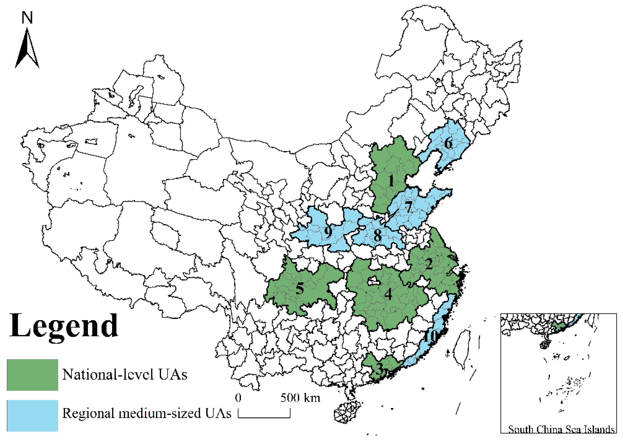
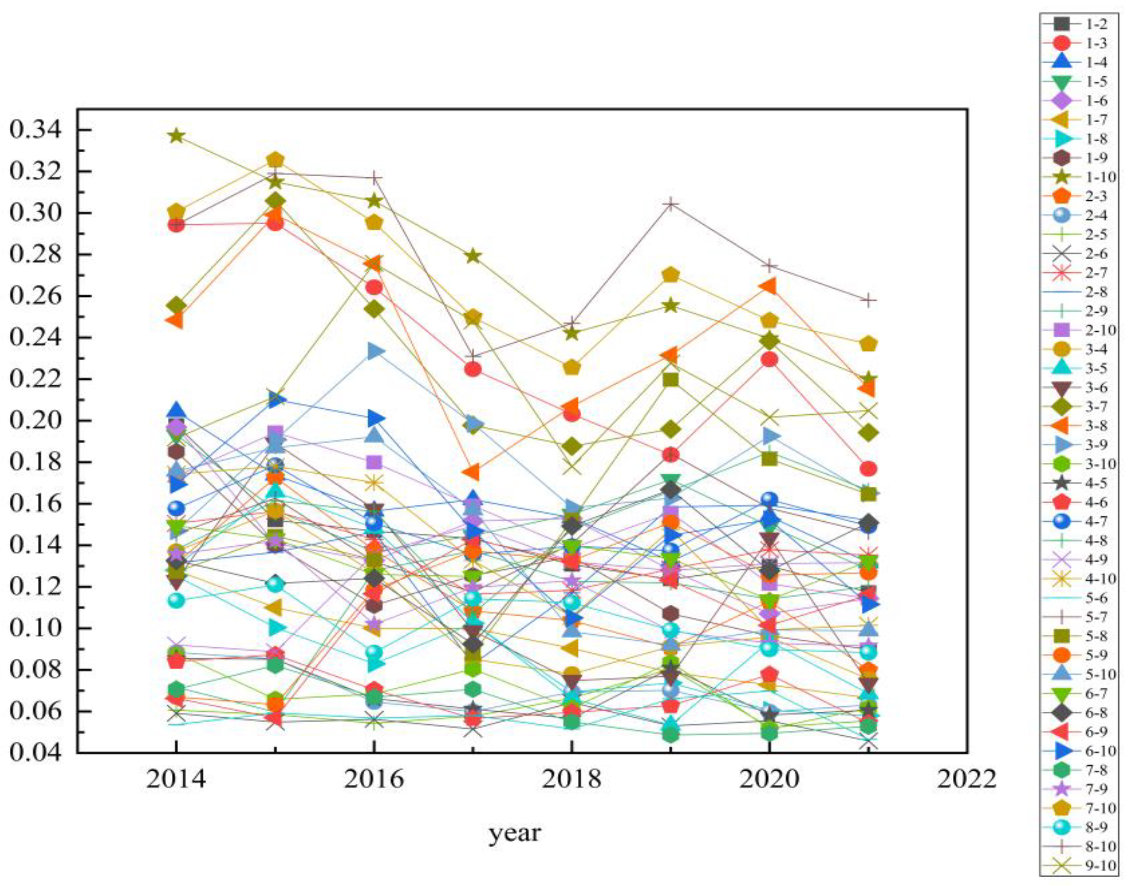
3.2.2. Differences in Air Quality between UAs

Dagum’s decomposition of the Gini coefficient of air quality among the ten UAs is shown in Figure 2. Among the regional differences in air quality, Beijing-Tianjin-Hebei and Pearl River Delta fluctuated the most in air quality, followed by that between Beijing-Tianjin-Hebei and Western Taiwan Strait. The regional differences between Chengdu-Chongqing and the Shandong Peninsula, between Chengdu-Chongqing and central and southern Liaoning, and between the Yangtze River Delta and Chengdu-Chongqing fluctuated less. The differences in air quality among most UAs showed a downward trend, among which Beijing-Tianjin-Hebei and Central Plains had the most significant decline, with an average annual decline of 10.42%. The differences between it and Guanzhong Plain, central and southern Liaoning and Guanzhong Plain, and Yangtze River Delta and Guanzhong Plain expanded, with an average annual growth rate of 9.54%, 8.33%, and 7.66%, respectively. Generally, there were specific differences in air quality among the ten UAs.

3.2.3. Overall Difference and Decomposition of Air Quality

Table 4. Dagum’s decomposition of Gini coefficient of air quality in the UAs.

Year	Overall	Intra-Regional		Inter-Regional		Intensity of Transvariation
		Source	Contribution Rate (%)	Source	Contribution Rate (%)	Source	Contribution Rate (%)
2014	0.1332	0.0091	6.8943	0.0944	71.4669	0.0286	21.6388
2015	0.1338	0.0089	6.6828	0.0990	74.5721	0.0249	18.7451
2016	0.1251	0.0076	6.0876	0.0953	76.5557	0.0216	17.3567
2017	0.1121	0.0072	6.4924	0.0812	72.9369	0.0229	20.5708
2018	0.1116	0.0072	6.5502	0.0803	72.6891	0.0229	20.7608
2019	0.1189	0.0071	6.0404	0.0932	78.9577	0.0177	15.0020
2020	0.1151	0.0063	5.5079	0.0942	82.3444	0.0139	12.1477
2021	0.1077	0.0066	6.1811	0.0840	78.4823	0.0164	15.3366
Mean	0.1197	0.0075	6.3046	0.0902	76.0006	0.0211	17.6948

shows the overall Gini coefficient and decomposition results of air quality in the ten UAs. The table also demonstrates the source and contribution of air quality differences in each UA. The overall difference in air quality showed a fluctuating downward trend, and the overall difference narrowed, with a Gini coefficient of 0.1332–0.1077. The coefficient reached the maximum value of 0.1338 in 2015, fluctuated and decreased after 2015, increased slightly in 2019, and finally fell to the minimum value of 0.1077 in 2021, with a decrease of 2.99%. The contribution of inter-regional differences in air quality was much higher than that of intra-regional differences and intensity of transvariation, indicating that inter-regional differences were the primary source of overall differences, accounting for 71.4669–82.3444%. The contribution rate of the intensity of transvariation was between 12.1477 and 21.6388%, representing the second most prominent source of overall differences. The contribution of intra-regional differences was the lowest, ranging from 5.5079% to 6.8943%. Judging from the evolution trend of the sources of differences, the contribution of inter-regional differences stood at 71.4669% in 2014 and then showed a fluctuating upward trend until it reached 78.4832% in 2021, with an average annual growth rate of 1.347%, suggesting that the differences between UAs widened. The intensity of transvariation was used to identify the overlap between UAs. Its contribution fluctuated and declined from 21.6388% in 2014 to 15.3366% in 2021, with an average annual decrease of 4.80%, showing that the overlap between UAs weakened, and the difference in air quality decreased. The contribution of intra-regional differences did not witness significant change and remained around 6.5%. It decreased year by year from 2014 to 2020, with a slight increase in 2021, indicating that the overall air quality in the UAs was relatively stable.

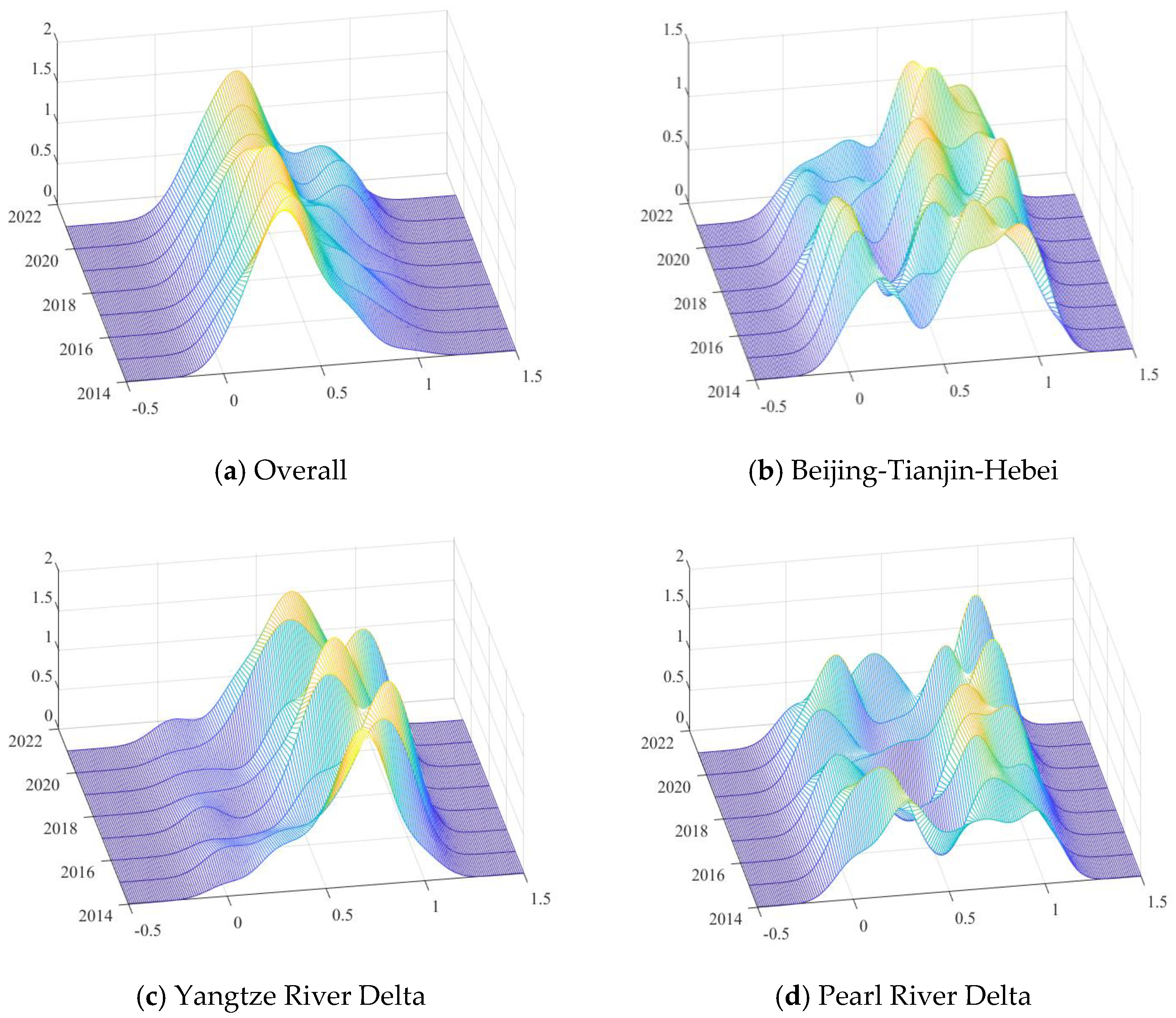
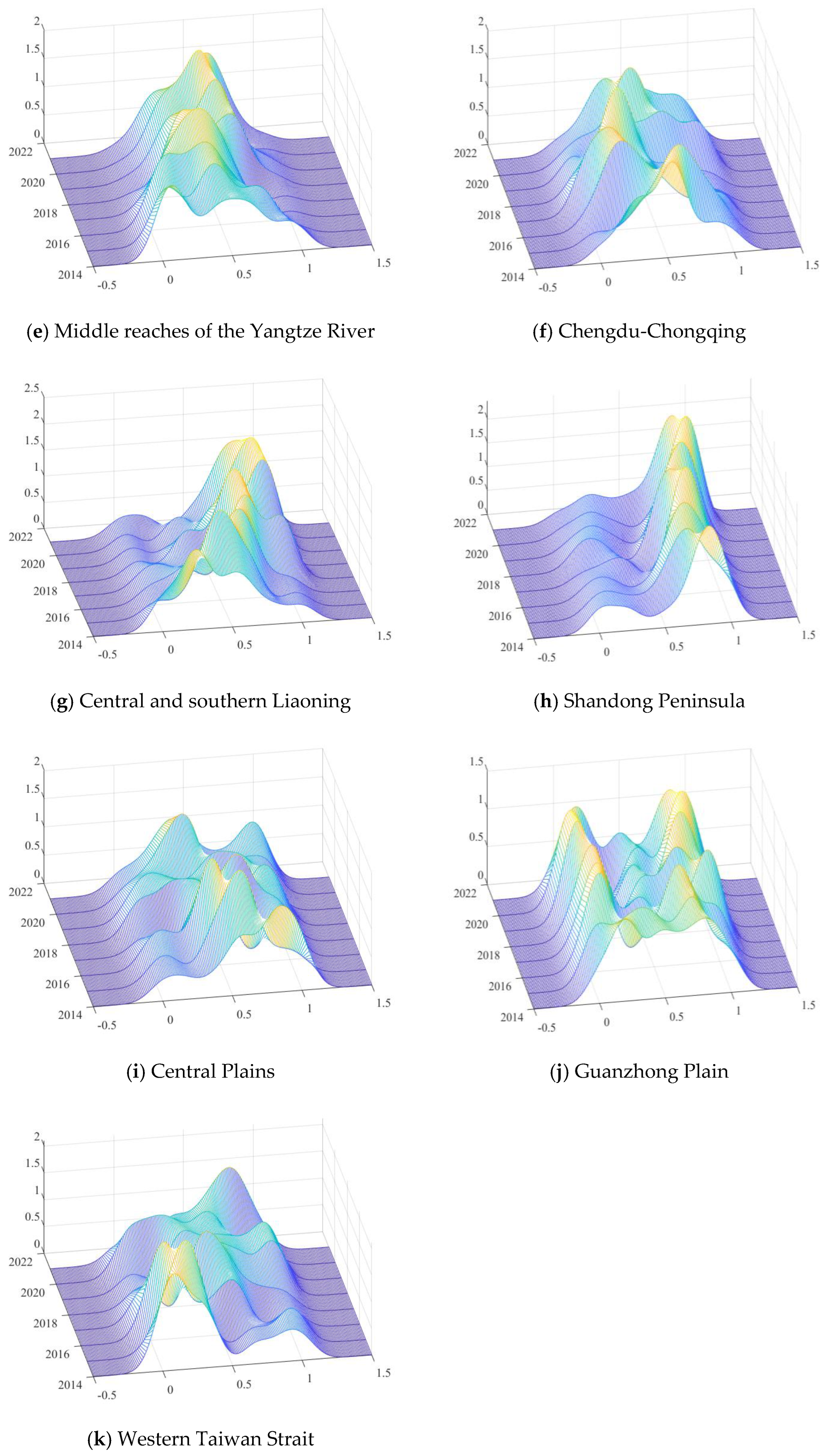
3.3. Distribution Dynamics of Air Quality

The Gini coefficient presented the size and source of air quality differences in UAs, reflected the relative differences in air quality and could describe the dynamic changes in absolute air quality differences. Therefore, the kernel density estimation was adopted to analyze the distribution dynamics of the air quality of the ten UAs as a whole as well as each of them in terms of the distribution location, pattern, ductility, and polarization. Figure 3 presents the results of the KDE.

The distribution location reflects the air quality. From 2014 to 2021, the center of the kernel density distribution curve of the ten UAs as a whole and Beijing-Tianjin-Hebei, Pearl River Delta, the middle reaches of the Yangtze River, central and southern Liaoning, Shandong Peninsula, Guanzhong Plain, and Western Taiwan Strait move rightward, indicating that the air quality of the ten UAs as a whole and several individual UAs improved with an upward trend. The center of the kernel density distribution curve in Beijing-Tianjin-Hebei, Pearl River Delta, central and southern Liaoning, and the Shandong Peninsula moved rightward remarkably, showing an apparent upward trend in air quality. In contrast, the curve of the Yangtze River Delta, Chengdu-Chongqing, and Central Plains moved leftward, indicating that their air quality declined. Generally, the overall air quality of UAs improved, demonstrating that China’s environmental protection has been effective.

The distribution pattern reflects the spatial difference and polarization of air quality in each UA. Specifically, the height and width of the wave crests reflect the difference, and the number of wave crests reflects the polarization. From the distribution pattern, the overall main peak of the ten UAs showed a change of “fall-rise-fall-rise”. The overall peak height decreased, and the width of the main peak continued to increase, indicating that the degree of internal dispersion was on the rise. The height of the main peak of Beijing-Tianjin-Hebei continued to rise, but the change in width was not prominent; the height of the Yangtze River Delta did not see much change, and the overall height showed a slight downward trend, with insignificant changes in width; the height of Pearl River Delta was rising, but the change in width was not noticeable; the height of the middle reaches of the Yangtze River increased, while the width decreased; the height of Chengdu-Chongqing decreased, but the width did not change significantly; the height of central and southern Liaoning increased, whereas the width was small; the height of Shandong Peninsula rose, but the width witnessed no remarkable change; the height of Central Plains fell, while the change in width was not apparent; the height of Guanzhong Plain increased, while the width did not change significantly; while the height of Western Taiwan Strait decreased, and the change of the width was reduced.

The distribution ductility reflects spatial differences in air quality. From the distribution ductility, Yangtze River Delta, central and southern Liaoning, and Central Plains showed a left-trailing phenomenon, while the ten UAs as a whole and some individual UAs displayed a right-trailing phenomenon. The air quality difference within the ten UAs as a whole and Guanzhong Plain tended to widen, while other UAs showed a convergence trend, suggesting that the air quality gap within these UAs was constantly narrowing.

From the perspective of polarization characteristics, the kernel density distribution curves of the ten UAs as a whole and each individual UA consisted of double peaks or multiple peaks, indicating that the air quality was multi-polarized to some extent, although there were some differences. The ten UAs as a whole changed from a single peak to multiple peaks, gradually showing polarization, and the distance between the main peak and the side peaks was small, showing slight differences within the UAs. The Shandong Peninsula showed pronounced double peaks from 2014 to 2021, and the distance between the two peaks was close, indicating minor differences within the UAs. However, there was a significant difference between the heights of the main peaks and side peaks of the ten UAs as a whole and the Shandong Peninsula, and the air quality within the UA was significantly different. The phenomenon of multiple peaks was common in other UAs. The difference in the heights between the peaks in UAs, such as Beijing-Tianjin-Hebei, Pearl River Delta, the middle reaches of the Yangtze River, Chengdu-Chongqing, Central Plains, Guanzhong Plain, and Western Taiwan Strait, was relatively small, and the air quality gap within the UA was also small.

3.4. Convergence Analysis of Air Quality

3.4.1. σ-Convergence

Table 5. σ-convergence Gini coefficient of air quality in the UAs.

Year	Overall	Beijing-Tianjin-Hebei	Yangtze River Delta	Pearl River Delta	The Middle Reaches of the Yangtze River	Chengdu-Chongqing	Central and Southern Liaoning	Shandong Peninsula	Central Plains	Guanzhong Plain	Western Taiwan Strait
2014	0.2415	0.2562	0.1192	0.1505	0.1825	0.1023	0.0926	0.1585	0.0801	0.1312	0.1327
2015	0.2394	0.2196	0.1021	0.1038	0.1803	0.1111	0.1000	0.1769	0.1156	0.1073	0.1314
2016	0.2221	0.1926	0.0975	0.1002	0.1292	0.0985	0.1025	0.1669	0.0731	0.2019	0.1049
2017	0.2033	0.1936	0.0958	0.1250	0.1037	0.1114	0.0964	0.1471	0.0860	0.2517	0.0884
2018	0.1981	0.1739	0.1144	0.1035	0.1148	0.0853	0.0989	0.1522	0.0331	0.2571	0.0677
2019	0.2102	0.1644	0.1114	0.1087	0.1403	0.0825	0.0804	0.1165	0.0438	0.2146	0.0533
2020	0.2044	0.1444	0.0840	0.1130	0.1185	0.0922	0.0878	0.1281	0.0471	0.1905	0.0571
2021	0.1919	0.1158	0.1020	0.1013	0.1212	0.0929	0.0657	0.1220	0.0623	0.1926	0.0727

shows the $\sigma$-convergence results of the air quality of the ten UAs as a whole and each individual UA. The overall air quality variation coefficient of the ten UAs decreased from 0.2415 in 2014 to 0.1919 in 2018, slightly increased to 0.2102 in 2019, showed a downward trend from 2019, and finally decreased to 0.1919 in 2021. Among the UAs, the coefficient of variation of Guanzhong Plain fluctuated and increased from 0.1312 in 2014 to 0.1926 in 2021, with an average annual increase of 5.6%. The other UAs showed a fluctuating downward trend, among which Western Taiwan Strait saw the most remarkable decline, with an average annual decrease of 8.24%. Generally speaking, the coefficient of variation of air quality in Guanzhong Plain increased without $\sigma$-convergence; the variation coefficient of the ten UAs as a whole and each individual UA showed a downward trend, all with $\sigma$-convergence. The air quality of each urban agglomeration was balanced. The regional disparity within these UAs narrowed, and the air quality of each UA was even.

3.4.2. β-Convergence

(1)

Absolute β-Convergence

We screened the models by LM test, Hausman test, LR test, and Wald test, analyzed the absolute $\beta$-convergence of the air quality of the ten UAs as a whole and each individual UA, and determined the convergence analysis model accordingly. After testing, Beijing-Tianjin-Hebei, Pearl River Delta, Chengdu-Chongqing, Shandong Peninsula, and Central Plains were shown to require a return to the traditional convergence model (

Table 6. Absolute $\beta$-convergence test of air quality in the UAs.

Area	Overall	Beijing-Tianjin-Hebei	Yangtze River Delta	Pearl River Delta	The Middle Reaches of the Yangtze River	Chengdu-Chongqing	Central and Southern Liaoning	Shandong Peninsula	Central Plains	Guan-Zhong Plain	Western Taiwan Strait
Model	Two-way fixed SDM	Two-way fixed OLS	Two-way fixed SAR	Two-way fixed OLS	Two-way fixed SDM	Two-way fixed OLS	Two-way fixed SAR	Two-way fixed OLS	Two-way fixed OLS	Two-way fixed SEM	Two-way fixed SAR
$\beta$	−0.6836 *** (−26.29)	−0.3396 *** (−5.31)	−0.6685 *** (−11.49)	−1.0544 *** (−8.83)	−0.7488 *** (−14.22)	−0.2769 *** (−4.48)	−0.8017 *** (−10.15)	−0.4120 *** (−5.90)	−0.6237 *** (−6.31)	−0.5600 *** (−6.25)	−0.6182 *** (−6.56)
$\theta$	0.3602 *** (8.60)				0.5511 *** (5.55)
$\rho$ or $\lambda$	0.4251 *** (14.26)		0.4465 *** (6.67)		0.4797 *** (6.56)		−0.2383 ** (−2.17)			0.2631 * (1.87)	−0.2156 ** (−2.28)
R2	0.2780	0.2677	0.1432	0.5954	0.3149	0.1742	0.1945	0.2562	0.3408	0.3961	0.4270
Log-L	1754.4811		365.5720		364.5399		192.8965			115.7514	133.9820
Space fixed effect	257.97 ***	52.64 ***	113.70 ***	45.53 ***	52.46 ***	42.52 ***	117.55 ***	58.27 ***	34.40 ***	33.13 ***	43.54 ***
Time fixed effect	520.53 ***	22.63 ***	99.68 ***	35.97 ***	116.56 ***	45.03 ***	67.93 ***	33.85 ***	21.88 ***	35.89 ***	23.65 ***
Hausman test	141.00 ***	8.72 ***	119.96 ***	25.79 ***	22.66 ***	5.78 **	111.93 ***	18.88 ***	9.61 **	46.11 ***	16.45 ***
LM (SAR)	788.946 ***	52.436 ***	229.000 ***	52.867 ***	197.990 ***	97.714 ***	71.577 ***	109.267 ***	52.647 ***	63.4000 ***	8.386 ***
R-LM (SAR)	0.274	2.040	0.100	13.129 ***	0.282	0.202	0.140	0.053	0.216	2.634	1.433
LM (SEM)	825.689 ***	51.994 ***	237.974 ***	40.230 ***	214.203 ***	104.723 ***	77.903 ***	110.588 ***	60.323 ***	60.781 ***	6.984 ***
R-LM (SEM)	37.016 ***	1.598	9.074 **	0.492	16.495 ***	7.212 ***	6.466 **	1.375	7.891 ***	0.015	0.031

***, **, and * indicate significance at the 1%, 5%, and 10% levels, respectively, with t value in brackets, the same below.

).

The ten UAs as a whole and the middle reaches of the Yangtze River partially passed the LM test, significantly passed the LR test and Wald test, and supported the SDM (this study did not report the LR test and Wald test for the SDM, which was available for retrieval). The spatial lag coefficient $\rho$ of the explained variables was significantly positive at a 1% level, indicating that the improved air quality in surrounding UAs promoted that of the target UA. The convergence coefficient was significantly negative at a 1% level, suggesting that the overall air quality of the ten UAs had an absolute $\beta$-convergence trend. $\theta$ was significantly positive, which means that the improved air quality in surrounding UAs substantially promoted that of the target UA. These findings revealed that spatial spillover was one of the critical factors in improving regional air quality.

Beijing-Tianjin-Hebei, Pearl River Delta, Chengdu-Chongqing, Shandong Peninsula, and Central Plains passed the LR and Wald tests, and some results failed the significance tests. In addition, after running SEM and SAR for Beijing-Tianjin-Hebei, Pearl River Delta, Chengdu-Chongqing, and the Shandong Peninsula, $\rho$ or $\lambda$ were shown to be not significant, and the SAR and SEM were shown to require a return to the traditional convergence model.

The spatial error coefficient $\lambda$ of central and southern Liaoning and Western Taiwan Strait was negative and passed the 1% significance test, showing a certain degree of negative spatial correlation, which means that a “core-periphery” pattern characterized air quality improvement. There was a competitive relationship between the cities within the UA, but the areas with relatively poor air quality were shown to consistently catch up, and the central city had a siphon effect. There was a positive spatial correlation between the Yangtze River Delta and Guanzhong Plain, suggesting that the improvement of surrounding air quality boosted the air quality of the target area.

The convergence coefficient $\beta$ of the UAs as a whole and each individual UA was negative and passed the 1% significance test, with an absolute $\beta$-convergence trend. Combining the spatial correlation and the convergence coefficient $\beta$, it could be seen that the spatial correlation of the UAs as a whole and each individual UA was one of the factors leading to the absolute $\beta$-convergence. While there was a significant negative spatial correlation between the central and southern Liaoning and Western Taiwan Strait, the absolute $\beta$-convergence still existed, indicating that the behindhand cities within the UA had strong momentums to catch up with cities ahead of them, and the air quality between cities was increasingly competitive.

(2)

Conditional $\beta$-Convergence

The convergence of air quality in UAs was further explored by considering five control variables: population, technological progress, government financial resources, economic development, and industrial structure. According to the convergence analysis steps, the conditional $\beta$-convergence analysis models of the ten UAs as a whole and each individual UA were respectively determined. After comparing the results of each model, the traditional convergence model was finally selected. The results are shown in

Table 7. Conditional $\beta$-convergence test of air quality in the UAs.

Area	Overall	Beijing-Tianjin-Hebei	Yangtze River Delta	Pearl River Delta	The Middle Reaches of the Yangtze River	Chengdu-Chongqing	Central and Southern Liaoning	Shandong Peninsula	Central Plains	Guanzhong Plain	Western Taiwan Strait
$\beta$	−0.8172 *** (−26.92)	−0.8026 *** (−7.86)	−1.0159 *** (−12.85)	−1.1815 *** (−9.65)	−1.0406 *** (−14.69)	−0.9857 *** (−9.44)	−0.6289 *** (−6.24)	−0.8213 *** (−8.31)	−0.9052 *** (−7.64)	−0.9685 *** (−7.39)	−0.8641 *** (−7.24)
X1	−0.0691 (−1.06)	0.0398 * (0.14)	−0.3591 *** (−3.57)	−0.2754 (−0.78)	−0.3830 * (−1.76)	0.0771 (0.32)	0.3026 (1.31)	−0.1425 (−0.49)	−0.4329 (−1.22)	0.0365 (0.12)	0.3157 (0.80)
X2	0.0097 (1.28)	−0.0413 (−1.37)	0.0281 (0.84)	0.0688 (1.40)	−0.0290 (−1.27)	−0.0397 * (−1.86)	0.0308 * (−0.92)	0.0126 (0.52)	0.0069 (0.18)	−0.0064 (−0.14)	−0.0265 (−1.32)
X3	−0.0344 (−1.44)	−0.1009 (−1.23)	−0.1551 ** (−2.47)	0.0478 (0.33)	0.1415 *** (2.69)	−0.0158 (−0.13)	−0.0502 (−0.92)	−0.2694 * (−1.89)	−0.0921 (−0.50)	0.0324 (0.28)	−0.0979 (−0.96)
X4	−0.2050 *** (−8.32)	−0.1186 (−1.19)	−0.3206 *** (−6.22)	−0.3020 * (−1.79)	−0.3785 *** (−5.81)	−0.3991 *** (−3.49)	−0.0209 (−0.23)	−0.0983 (−1.30)	−0.1807 (−0.99)	−0.3080 ** (−2.26)	−0.0129 (−0.16)
X5	0.3617 *** (10.88)	0.3079 *** (3.36)	0.2050 ** (2.09)	0.3428 (0.97)	0.2310 ** (2.13)	0.2527 (1.55)	0.2504 *** (2.97)	0.3874 *** (4.10)	0.0051 (0.03)	0.1234 (0.66)	0.0826 (0.47)
R2	0.4386	0.4852	0.5270	0.6640	0.5802	0.5078	0.3816	0.4631	0.4690	0.4969	0.4950

***, **, and * indicate significance at the 1%, 5%, and 10% levels, respectively, with t value in brackets, the same below.

. The conditional convergence coefficients of the air quality of the ten UAs as a whole and each individual UA were all negative and passed the 1% significance test, indicating a trend of conditional convergence.

The regression coefficients of the control variables showed that in the ten UAs, the two variables X4 and X5 passed the significance level test and had a significant impact on the conditional $\beta$-convergence of the AQI, while X1, X2, and X3 did not pass the significance level test and had no significant effect on the convergence of the AQI. The influence of X5 was significantly positive, suggesting that the industrial structure could improve the air quality in UAs but had a particular inhibitory effect on narrowing the AQI gap between UAs. The gap in industrial structure was the main factor for the gap in air quality between UAs.

For each UA, the control variables, such as X1, X2, X3, X4, and X5, had different effects on improving the air quality. For example, X3 had a significant positive impact on the air quality of the middle reaches of the Yangtze River. The improvement of X3 substantially promoted the air quality of the middle reaches of the Yangtze River, but it had an inhibitory effect on narrowing the gap within the UA. Therefore, to improve the air quality of the UA, it is necessary for government financial resources to play a role, to optimize the allocation of resources, and improve people’s living standards. X3 had a significant negative impact on the air quality of the Yangtze River Delta and had a promoting effect on reducing the air quality gap in the UA. However, it had no significant impact on the air quality of other UAs, Yangtze River Delta, and the middle reaches of the Yangtze River. Therefore, it is necessary to utilize the government’s financial resources further to improve resource allocation, optimize the environment, and pay attention to the impact on the air quality gap within the UA.

3.4.3. Club Convergence

Dagum’s decomposition of the Gini coefficient revealed that the air quality difference between UAs was an essential source of the overall difference. We conducted a club convergence test based on UAs at different levels to further examine the air quality difference between UAs. The absolute and conditional $\beta$-convergence test results of air quality in UAs at the two levels are shown in

Table 8. Club convergence test of air quality in the UAs.

	$\mathbf{Absolute}\mathit{\beta }$-Converg		$\mathbf{Conditional}\mathit{\beta }$-Converg
Area	First Layer	Second Layer	First Layer	Second Layer
Model	Two-Way Fixed SEM	Two-Way Fixed SEM	Two-Way Fixed SDM	Two-Way Fixed SEM
$\beta$	−0.6172 *** (−20.01)	−0.7019 *** (−17.09)	−0.6425 *** (−20.60)	−0.7154 *** (−17.52)
$\theta$			0.2247 *** (4.10)
ρ or λ	0.5159 *** (14.39)	0.2463 *** (5.11)	0.4839 *** (12.84)	0.2369 *** (4.85)
X1			0.08830 * (1.76)	0.0727 (0.89)
X2			−0.0139 ** (−2.01)	0.0056 (0.78)
X3			−0.0146 (−0.74)	−0.0204 (−0.70)
X4			0.0444 (1.38)	0.0861 *** (2.64)
X5			0.0525 (1.44)	−0.0207 (−0.48)
R2	0.2503	0.3008	0.3135	0.2686
Log-L	1133.4696	669.7970	1151.7943	675.6161
Space fixed effect	154.00 ***	147.82 ***	95.42 ***	148.18 ***
Time fixed effect	272.98 ***	224.09 ***	297.57 ***	232.87 ***
Hausman test	284.23 ***	269.66 ***	60.98 ***	289.99 ***
LM spatial lag	639.470 ***	195.079 ***	642.784 ***	191.207 ***
Robust LM spatial lag	0.324	1.540	1.929	0.520
LM spatial error	686.177 ***	207.926 ***	677.778 ***	203.645 ***
Robust LM spatial error	47.031 ***	14.387 ***	36.924 ***	12.958 ***

***, **, and * indicate significance at the 1%, 5%, and 10% levels, respectively, with t value in brackets, the same below.

. The absolute club convergence coefficients of UAs at different levels were significantly negative, and the air quality among UAs at the same level was characterized by absolute $\beta$-convergence. With development of the economy, the communication between UAs has become increasingly close. The significant positive spatial correlation between UAs at different levels strengthened their connection and enhanced the absolute $\beta$-convergence trend.

After adding the relevant control variables, the conditional $\beta$-convergence coefficients of AQI of UAs at the two levels were significantly negative, and the air quality within UAs at different levels had a conditional $\beta$-convergence trend. There were spatial correlations within the UAs at the first level, including Yangtze River Delta, Pearl River Delta, and Beijing-Tianjin-Hebei. The spatial effect accounted for the conditional $\beta$-convergence trend in UAs at the first level, indicating that the interaction between high-level UAs was tighter. The influence of each control variable in UAs at different levels was different. For example, economic development was not significant in the first layer but significantly positive in the second layer. Therefore, the impact of each variable on the air quality of UAs varied from region to region.

4. Conclusions and Policy Implications

4.1. Conclusions

This study measured the air quality of ten UAs in China based on the AQI from 2014 to 2021. We analyzed, estimated, and decomposed the regional differences using Dagum’s decomposition of the Gini coefficient, described the distribution dynamics using kernel density estimation, and tested the $\sigma$-convergence, $\beta$-convergence, and club convergence. The conclusions drawn were as follows:

(1) According to the AQI from 2014 to 2021, there were spatiotemporal differences in the air quality of the ten UAs in China: from the scale of time, the AQI of each UA showed a downward trend over the years; from the perspective of space, the overall AQI of UAs was high in the north and low in the south. In other words, the air quality of China’s UAs gradually improved, and the air quality in the south was better than that in the north.

(2) Dagum’s decomposition of the Gini coefficient demonstrated no significant difference in air quality within each UA, but there was a particular gap in air quality between UAs. Among them, the air quality difference between Beijing-Tianjin-Hebei and Pearl River Delta was the largest; the overall air quality difference in the UAs showed a decreasing trend; and the regional difference in air quality was the primary source of the overall difference in air quality.

(3) In the distribution dynamics of the air quality estimated by kernel density estimation, the overall distribution curve of the ten UAs moved rightward, and the air quality of the UAs improved to a certain extent. The changing trend of height and width of the ten UAs as a whole and each individually were inconsistent. Except for the left-tailing phenomenon in the Yangtze River Delta, central and southern Liaoning, and Central Plains, the ten UAs as a whole and the other UAs showed a right-tailing phenomenon, but the ductility of the distribution curves was different. The kernel density estimation curves of the ten UAs as a whole and each individually consisted of double or multiple peaks, indicating that air quality was multi-polarized to some extent.

(4) The convergence model demonstrated that except for Guanzhong Plain, the air quality of the UAs as a whole and each of the other UAs featured $\sigma$-convergence, and the ten UAs as a whole and each individually had absolute and conditional $\beta$-convergence. In addition, the air quality in UAs at different levels was characterized by club convergence.

In the future, spatial autocorrelation analysis and standard deviation ellipse can be used to systematically analyze the regional differences in air quality, and the spatial econometric model and Geodetector can be used to analyze the influencing mechanism of the air quality of UAs.

4.2. Policy Implications

(1) It is necessary to constantly improve the air quality of China’s UAs. This study shows that the AQI of each UA in China displays a downward trend over time, indicating that the air quality of each UA has improved to some extent, but still needs to be further improved. Improving air quality is a response to environmental protection and green development nowadays. Since there is still extensive resource utilization in China’s UAs, it remains necessary to establish the concept of green development, rationally allocate resources, improve energy efficiency, reduce pollution emissions in industrial production, and improve air quality in UAs by both the government and the market.

(2) For UAs with significant internal differences in air quality, their central cities should continue to improve resource allocation and utilization efficiency through the agglomeration effect, strengthen the radiation and driving effect within the UA, and improve the overall air quality of the UA. It is crucial for other UAs with shrinking differences to further achieve regional coordination and overall prosperity within each UA. The development of each UA should fully consider each city’s resource endowment and location advantages to avoid further increases in air quality differences.

(3) The Gini coefficient shows that regional differences are the primary source of the overall differences in air quality. There is a significant difference between Beijing-Tianjin-Hebei and Pearl River Delta and between Beijing-Tianjin-Hebei and Western Taiwan Strait due to the geographical differences between the north and the south. Therefore, the overall AQI in China’s UAs is high in the north and low in the south. To this end, Beijing-Tianjin-Hebei, Shandong Peninsula, and other northern UAs should strive to build ecological cities while continuing to develop their economies, and should continue to strengthen the control of air pollutant emissions and reduce energy consumption in industrial production activities. The extensive utilization of resources should be addressed by the rational allocation of resources to avoid waste of resources in the production process, establish a green and intensive development concept, improve the air quality of various UAs in China, and vigorously promote the construction of an ecological culture and the overall air quality of UAs. For southern UAs with better air quality, it is also essential to build effective channels for cooperation and communication between UAs so that UAs with poor air quality can extensively learn from the regions with better air quality.

(4) There are absolute and conditional $\beta$-convergence trends in China’s UAs, indicating that the differences in air quality among China’s UAs are narrowing. China has a vast territory with different resource endowments and economic development levels, and it is not easy to achieve a balanced development that is entirely undifferentiated in terms of air quality. However, to improve the air quality of UAs as a whole, it is still necessary to improve the air quality in cities with poor air quality, strengthen the concept of green development, and protect the atmospheric environment. It is also essential to strengthen the overall coordination of the region and promote the overall improvement of air quality in China’s UAs. For Beijing–Tianjin–Hebei, Yangtze River Delta, and Pearl River Delta, the three most developed UAs in China, it is necessary to further improve the quality of development to drive national economic growth and improve air quality. The Yangtze River Delta and Chengdu Chongqing need to drive the central and western parts of China, respectively, to improve air quality. The other five regional UAs need to integrate green and innovative elements into the development process, and pay attention to the coordination of economic growth and environmental protection.

In short, the air quality of China’s UAs needs to be further improved. The central government should play a crucial role in addressing the current air pollution problems in UAs. Legal and administrative means can be used to strengthen the supervision and management of air pollution, and green finance can also be used to encourage energy conservation, environmental protection, and technological development. Like all industrialized countries, China’s industrialization is accompanied by air pollution. In the future, UAs need to promote cleaner production methods, energy-saving and environmental protection technologies, transform those industries with high pollution and high energy consumption, and further improve the air quality of China’s UAs.

References

1. Li, C.Y.; Zhang, Y.M.; Zhang, S.Q. Applying the Super-EBM model and spatial Durbin model to examining total-factor ecological efficiency from a multi-dimensional perspective: Evidence from China. Environ. Sci. Pollut. Res. 2022, 29, 2183–2202. [Google Scholar] [CrossRef]
2. Tu, Z.G.; Hu, T.Y.; Shen, R.J. Evaluating public participation impact on environmental protection and ecological efficiency in China: Evidence from PITI disclosure. China Econ. Rev. 2019, 55, 111–123. [Google Scholar] [CrossRef]
3. Feng, D.; Zhang, Y.Q.; Zhang, X.Y. Applying a data envelopment analysis game cross-efficiency model to examining regional ecological efficiency: Evidence from China. J. Clean. Prod. 2020, 267, 122031. [Google Scholar] [CrossRef]
4. Chen, S.Y.; Chen, D.K. Air Pollution, Government regulations and high-quality economic development. Econ. Res. J. 2018, 53, 20–34. [Google Scholar]
5. Wang, Z.Y.; Shi, X.Y.; Pan, C.H.; Wang, S.S. Spatial and temporal characteristics of environmental air Quality and its relationship with seasonal climatic conditions in Eastern China during 2015–2018. Int. J. Environ. Res. Public Health 2021, 18, 4524. [Google Scholar] [CrossRef] [PubMed]
6. Bandh, S.A.; Shafi, S.; Peerzada, M.; Rehman, T.; Bashir, S.; Wani, S.A.; Dar, R. Multidimensional analysis of global climate change: A review. Environ. Sci. Pollut. Res. 2021, 28, 24872–24888. [Google Scholar] [CrossRef]
7. Zhou, D.; Lin, Z.L.; Liu, L.M.; Liu, L.M.; Qi, J.L. Spatial-temporal characteristics of urban air pollution in 337 Chinese cities and their influencing factors. Environ. Sci. Pollut. Res. 2021, 28, 36234–36258. [Google Scholar] [CrossRef]
8. Dong, D.; Xu, B.; Shen, N.; He, Q. The adverse impact of air pollution on China’s economic growth. Sustainability 2021, 13, 9056. [Google Scholar] [CrossRef]
9. Zheng, B.L.; Liang, L.T.; Li, M.M. Analysis of temporal and spatial patterns of PM2.5 in Prefecture-Level Cities of China from 1998 to 2016. China Environ. Sci. 2019, 39, 1909–1919. [Google Scholar] [CrossRef]
10. Li, M.S.; Zhang, J.H.; Zhang, Y.J.; Zhou, L.; Li, Q.; Chen, Y.H. Spatio-temporal pattern changes of ambient air PM10 pollution in China from 2002 to 2012. Acta Geogr. Sin. 2013, 68, 1504–1512. [Google Scholar] [CrossRef]
11. Xu, L.J.; Zhou, J.X.; Guo, Y.; Wu, T.M.; Chen, T.T.; Zhong, Q.J.; Yuan, D.; Chen, P.Y.; Ou, C.Q. Spatiotemporal pattern of air quality index and its associated factors in 31 Chinese provincial capital cities. Air Qual. Atmos. Health 2017, 10, 601–609. [Google Scholar] [CrossRef]
12. Tui, Y.; Qiu, J.X.; Wang, J.; Fang, C.S. Analysis of spatio-temporal variation characteristics of main air pollutants in Shijiazhuang City. Sustainability 2021, 13, 941. [Google Scholar] [CrossRef]
13. Chukwu, T.; Morse, S.; Murphy, R. Spatial analysis of air quality assessment in two cities in nigeria: A comparison of perceptions with instrument-based methods. Sustainability 2022, 14, 5403. [Google Scholar] [CrossRef]
14. Lin, X.Q.; Wang, D. Spatio-temporal variations and socio-economic driving forces of air quality in Chinese cities. Acta Geogr. Sin. 2016, 71, 1357–1371. [Google Scholar] [CrossRef]
15. Huang, C.H.; Liu, K.; Zhou, L. Spatio-temporal trends and influencing factors of PM2.5 concentrations in urban agglomerations in China between 2000 and 2016. Environ. Sci. Pollut. Res. 2021, 28, 10988–11000. [Google Scholar] [CrossRef]
16. Platikanov, S.; Terrado, M.; Pay, M.T.; Soret, A.; Tauler, R. Understanding temporal and spatial changes of O3 or NO2 concentrations combining multivariate data analysis methods and air quality transport models. Sci. Total Environ. 2022, 806, 150923. [Google Scholar] [CrossRef]
17. Batterman, S.; Ganguly, R.; Harbin, P. High resolution spatial and temporal mapping of traffic-related air pollutants. Int. J. Environ. Res. Public Health 2015, 12, 3646–3666. [Google Scholar] [CrossRef] [Green Version]
18. Mendez-Espinosa, J.F.; Rojas, N.F.; Vargas, J.; Pachón, J.E.; Belalcazar, L.C.; Ramírez, O. Air quality variations in Northern South America during the COVID-19 lockdown. Sci. Total Environ. 2020, 749, 141621. [Google Scholar] [CrossRef]
19. Liu, H.M.; Fang, C.L.; Huang, J.J.; Zhu, X.D.; Zhou, Y.; Wang, Z.B.; Zhang, Q. The spatial-temporal characteristics and influencing factors of air pollution in Beijing-Tianjin-Hebei urban agglomeration. Acta Geogr. Sin. 2018, 73, 177–191. [Google Scholar] [CrossRef]
20. Wang, Z.S.; Li, Y.T.; Chen, T.; Zhang, D.W.; Sun, F.; Pan, L.B. Spatial-temporal characteristics of PM2.5 in Beijing in 2013. Acta Geogr. Sin. 2015, 70, 110–120. [Google Scholar] [CrossRef]
21. Zhan, J.Y.; Huang, G.C.; Zhou, H.; Duan, W.S.; Wu, A.A.; Wang, W.J.; Li, T. Spatial and temporal distribution characteristics and factors of particulate matter concentration in North China. J. Nat. Resour. 2021, 36, 1036–1046. [Google Scholar] [CrossRef]
22. Arowosegbe, O.O.; Röösli, M.; Adebayo-Ojo, T.C.; Dalvie, M.A.; Hoogh, K. Spatial and temporal variations in PM10 concentrations between 2010–2017 in South Africa. Int. J. Environ. Res. Public Health 2021, 18, 13348. [Google Scholar] [CrossRef] [PubMed]
23. Farsani, M.H.; Shirmardi, M.; Alavi, N.; Maleki, H.; Sorooshian, A.; Babaei, A.; Asgharnia, H.; Marzouni, M.B.; Goudarzi, G. Evaluation of the relationship between PM10 concentrations and heavy metals during normal and dusty days in Ahvaz, Iran. Aeolian Res. 2018, 33, 12–22. [Google Scholar] [CrossRef]
24. Xie, J.Y.; Suh, D.H.; Joo, S. Dynamic analysis of air pollution: Implications of economic growth and renewable energy consumption. Int. J. Environ. Res. Public Health 2021, 18, 9906. [Google Scholar] [CrossRef] [PubMed]
25. Shi, T.; Liu, M.; Hu, Y.M.; Li, C.L.; Zhang, C.Y.; Ren, B.H. Spatiotemporal pattern of fine particulate matter and impact of urban socioeconomic factors in China. Int. J. Environ. Res. Public Health 2019, 16, 1099. [Google Scholar] [CrossRef] [PubMed] [Green Version]
26. Jing, B.; Ni, Z.Y.; Zhao, L.Y.; Liu, K. Does rural-urban income gap exacerbate or restrain air pollution. China Popul. Resour. Environ. 2021, 31, 130–138. [Google Scholar] [CrossRef]
27. Dinda, S.; Coondoo, D.; Pal, M. Air quality and economic growth: An empirical study. Ecol. Econ. 2000, 34, 409–423. [Google Scholar] [CrossRef]
28. Wu, Y.P.; Dong, S.C.; Song, J.F. Modeling economic growth and environmental degradation of Beijing. Geogr. Res. 2002, 21, 239–246. [Google Scholar] [CrossRef]
29. Peng, J.Y.; Zhang, Y.G.; Xie, R.; Liu, Y. Analysis of driving factors on China’s air pollution emissions from the view of critical supply chains. J. Clean. Prod. 2018, 203, 197–209. [Google Scholar] [CrossRef]
30. Zhang, R.L.; Mi, K.N. Energy consumption, structural changes and air quality: Empirical test based on inter-provincial panel data. Geogr. Res. 2022, 41, 210–228. [Google Scholar] [CrossRef]
31. Tan, X.; Yu, W.; Wu, S. The impact of the dynamics of agglomeration externalities on air pollution: Evidence from urban panel data in China. Sustainability 2022, 14, 580. [Google Scholar] [CrossRef]
32. Ma, L.M.; Zhang, X. The spatial effect of China’s haze pollution and the impact from economic change and energy structure. China Ind. Econ. 2014, 4, 19–31. [Google Scholar] [CrossRef]
33. He, L.Y.; Wu, M.; Wang, D.Q.; Zhong, Z.Q. A study of the influence of regional environmental expenditure on air quality in China: The effectiveness of environmental policy. Environ. Sci. Pollut. Res. 2018, 25, 7454–7468. [Google Scholar] [CrossRef] [PubMed]
34. Wang, F.; Yang, J.; Shackman, J.; Liu, X. Impact of income inequality on urban air quality: A game theoretical and empirical study in China. Int. J. Environ. Res. Public Health 2021, 18, 8546. [Google Scholar] [CrossRef] [PubMed]
35. Chen, B.; Yang, S.; Xu, X.D.; Zhang, W. The impacts of urbanization on air quality over the Pearl River Delta in winter: Roles of urban land use and emission distribution. Theor. Appl. Climatol. 2014, 117, 29–39. [Google Scholar] [CrossRef]
36. Bandeira, J.M.; Coelho, M.C.; Sá, M.E.; Tavares, R.; Borrego, C. Impact of land use on urban mobility patterns, emissions and air quality in a Portuguese medium-sized city. Sci. Total Environ. 2011, 409, 1154–1163. [Google Scholar] [CrossRef] [PubMed] [Green Version]
37. Sun, C.W.; Luo, Y.; Yao, X. The effects of transportation infrastructure on air quality: Evidence from empirical analysis in China. Econ. Res. J. 2019, 54, 136–151. [Google Scholar]
38. Guo, Y.J.; Zhang, Q.; Lai, K.K.; Zhang, Y.Q.; Wang, S.B.; Zhang, W.L. The impact of urban transportation infrastructure on air quality. Sustainability 2020, 12, 5626. [Google Scholar] [CrossRef]
39. Huang, Z.J.; Song, L.; Gao, B.Y.; Jiang, L. Industrial land transfer, industrial selection and urban air quality. Geogr. Res. 2022, 41, 229–250. [Google Scholar] [CrossRef]
40. Zhou, J.; Lan, H.; Zhao, C.; Zhou, J. Haze pollution levels, spatial spillover influence, and impacts of the digital economy: Empirical evidence from China. Sustainability 2021, 13, 9076. [Google Scholar] [CrossRef]
41. Jiang, L.; Zhou, H.F.; Bai, L. Spatial Heterogeneity Analysis of Impacts of Foreign Direct Investment on Air Pollution: Empirical Evidence from 150 Cities in China Based on AQI. Sci. Geogr. Sin. 2018, 38, 351–360. [Google Scholar] [CrossRef]
42. Wang, J.H.; Ogawa, S. Effects of Meteorological Conditions on PM2.5 Concentrations in Nagasaki, Japan. Int. J. Environ. Res. Public Health 2015, 12, 9089–9101. [Google Scholar] [CrossRef] [PubMed]
43. Wang, J.Y.; Zhang, H.R.; Zhao, X.W.; Ji, J.H.; Yang, S.Z. Variation of air quality index and its relationship with meteorological elements in Beijing from 2012 to 2015. Meteorol. Environ. Sci. 2017, 40, 35–41. [Google Scholar] [CrossRef]
44. Kang, H.Y.; Liu, Y.L.; Li, T. Characteristics of air quality index and its relationship with meteorological factors in key cities of Heilongjiang Province. J. Nat. Resour. 2017, 32, 692–703. [Google Scholar] [CrossRef]
45. Wang, T.H.; Du, H.D.; Zhao, Z.Z.; Zhou, Z.M.; Russo, A.; Xi, H.L.; Zhang, J.P.; Zhou, C.J. Prediction of the impact of meteorological conditions on air quality during the 2022 Beijing Winter Olympics. Sustainability 2022, 14, 4574. [Google Scholar] [CrossRef]
46. Tiziano, T.; Umberto, R. An analytical air pollution model for complex terrain. Environmetrics 1994, 5, 159–165. [Google Scholar] [CrossRef]
47. Yu, S.; Wang, C.; Liu, K.; Zhang, S.; Dou, W. Environmental effects of prohibiting urban fireworks and firecrackers in Jinan, China. Environ. Monit. Assess. 2021, 193, 512. [Google Scholar] [CrossRef]
48. Zhao, L.; Liu, C.; Liu, X.; Liu, K.; Shi, Y. Urban spatial structural options for air pollution control in China: Evidence from provincial and municipal levels. Energy Rep. 2021, 7, 93–105. [Google Scholar] [CrossRef]
49. Aleluia, R.; Drouet, L.; Dingenen, R.; Emmerling, J. Future global air quality indices under different socioeconomic and climate assumptions. Sustainability 2018, 10, 3645. [Google Scholar] [CrossRef] [Green Version]
50. Zhang, J.H.; Tian, P.L.; Liu, X.; Yang, Y.; Wang, K.; Wang, W.J. Effect of urban greening on air quality: Take 27 provincial capitals in China as an example. Bull. Bot. Res. 2019, 39, 471–480. [Google Scholar] [CrossRef]
51. Irga, P.J.; Burchett, M.D.; Torpy, F.R. Does urban forestry have a quantitative effect on ambient air quality in an urban environment? Atmos. Environ. 2015, 120, 173–181. [Google Scholar] [CrossRef] [Green Version]
52. Bai, L.; Jiang, L.; Zhou, H.F.; Chen, Z.S. Spatio-temporal characteristics of air quality index and its driving factors in the Yangtze River Economic Belt: An empirical study based on bayesian spatial econometric model. Sci. Geogr. Sin. 2018, 38, 2100–2108. [Google Scholar] [CrossRef]
53. Zhang, Y.Q.; Bash, J.O.; Roselle, S.J.; Shatas, A.; Repinsky, A.; Mathur, R.; Hogrefe, C.; Piziali, J.; Jacobs, T.; Gilliland, A. Unexpected air quality impacts from implementation of green infrastructure in urban environments: A Kansas City case study. Sci. Total Environ. 2020, 744, 140960. [Google Scholar] [CrossRef] [PubMed]
54. Zhou, Y.J.; Liu, H.L.; Zhou, J.X.; Xia, M. Simulation of the impact of urban forest scale on PM2.5 and PM10 based on system dynamics. Sustainability 2019, 11, 5998. [Google Scholar] [CrossRef] [Green Version]
55. Dagum, C. A new approach to the decomposition of the Gini income inequality ratio. Empir. Econ. 1997, 22, 515–531. [Google Scholar] [CrossRef]
56. Xiong, H.H.; Lan, L.Y.; Liang, L.W.; Liu, Y.B.; Xu, X.Y. Spatiotemporal differences and dynamic evolution of PM2.5 pollution in China. Sustainability 2020, 12, 5349. [Google Scholar] [CrossRef]
57. Zhang, Z.M.; Wang, X.Y.; Zhang, Y.; Nan, Z.; Shen, B.G. The over polluted water quality assessment of Weihe River based on Kernel Density Estimation. Procedia Environ. Sci. 2012, 13, 1271–1282. [Google Scholar] [CrossRef]
58. Liu, K.; Wang, X.Y.; Zhang, Z.B. Assessing urban atmospheric environmental efficiency and factors influencing it in China. Environ. Sci. Pollut. Res. 2022, 29, 594–608. [Google Scholar] [CrossRef]
59. Cui, E.; Ren, L.; Sun, H.Y. Evaluation of variations and affecting factors of eco-environmental quality during urbanization. Environ. Sci. Pollut. Res. 2015, 22, 3958–3968. [Google Scholar] [CrossRef]
60. Wang, W.T.; Zhang, L.J.; Zhao, J.; Qi, M.Q.; Chen, F.R. The effect of socioeconomic factors on spatiotemporal patterns of PM2.5 concentration in Beijing–Tianjin–Hebei region and surrounding areas. Int. J. Environ. Res. Public Health 2020, 17, 3014. [Google Scholar] [CrossRef]
61. Zhou, L.; Zhou, C.H.; Yang, F.; Che, L.; Wang, B.; Sun, D.Q. Spatio-temporal evolution and the influencing factors of PM2.5 in China between 2000 and 2015. J. Geogr. Sci. 2019, 29, 253–270. [Google Scholar] [CrossRef] [Green Version]
62. He, Z.F.; Guo, Q.C.; Liu, J.Z.; Zhang, Y.Y.; Liu, J.; Ding, H. Spatio-temporal variation characteristics of air pollution and influencing factors in Hebei province. J. Nat. Resour. 2021, 36, 411–419. [Google Scholar] [CrossRef]
63. Xiao, J.C.; Yuan, Z. China’s Top Ten Urban Agglomerations; Economic Science Press: Beijing, China, 2009. [Google Scholar]
64. Yazdani, M.; Baboli, Z.; Maleki, H.; Birgani, Y.T.; Zahiri, M.; Chaharmahal, S.S.H.; Goudarzi, M.; Mohammadi, M.J.; Alam, K.; Sorooshian, A.; et al. Contrasting Iran’s air quality improvement during COVID-19 with other global cities. J. Environ. Health Sci. Eng. 2021, 19, 1801–1806. [Google Scholar] [CrossRef] [PubMed]
Figure 1. Spatial distribution of the ten UAs in China.
Sustainability 14 07330 g001
Figure 2. Evolution of Gini coefficients among the ten UAs.
Sustainability 14 07330 g002
Figure 3. Distribution dynamics of air quality in UAs.
Sustainability 14 07330 g003aSustainability 14 07330 g003b