Application of Combined Models Based on Empirical Mode Decomposition, Deep Learning, and Autoregressive Integrated Moving Average Model for Short-Term Heating Load Predictions

Abstract

Short-term building energy consumption prediction is of great significance for the optimized operation of building energy management systems and energy conservation. Due to the high-dimensional nonlinear characteristics of building heat loads, traditional single machine-learning models cannot extract the features well. Therefore, in this paper, a combined model based on complete ensemble empirical mode decomposition with adaptive noise (CEEMDAN), four deep learning (DL), and the autoregressive integrated moving average (ARIMA) models is proposed. The DL models include a convolution neural network, long- and short-term memory (LSTM), bi-directional LSTM (bi-LSTM), and the gated recurrent unit. The CEEMDAN decomposed the heating load into different components to extract the different features, while the DL and ARIMA models were used for the prediction of heating load features with high and low complexity, respectively. The single-DL models and the CEEMDAN-DL combinations were also implemented for comparison purposes. The results show that the combined models achieved much higher accuracy compared to the single-DL models and the CEEMDAN-DL combinations. Compared to the single-DL models, the average coefficient of determination (R²), root mean square error (RMSE), and coefficient of variation of the RMSE (CV-RMSE) were improved by 2.91%, 47.93%, and 47.92%, respectively. Furthermore, CEEMDAN-bi-LSTM-ARIMA performed the best of all the combined models, achieving values of R2 = 0.983, RMSE = 70.25 kWh, and CV-RMSE = 1.47%. This study provides a new guide for developing combined models for building energy consumption prediction.

1. Introduction

Building energy consumption accounts for more than one-third of the global total energy consumption and is expected to continue increasing with the acceleration of urbanization in developing countries [1]. Consequently, energy saving and sustainable buildings have become the top priority of all countries in the world. To solve this problem, researchers have put forward a series of building energy-saving measures, such as renewable energy utilization and high-performance building envelopes. Among them, efficient intelligent control is one of the most effective measures to reduce energy consumption during the building’s lifecycle [2]. However, building energy consumption exhibits substantial randomness, so its accurate and reliable prediction is of great significance to predictive building systems’ control and optimal scheduling [3,4,5].

Depending on the time-scale range, building energy consumption prediction (BECP) methods can be divided into short-term, medium-term, and long-term [6]. Short-term building energy forecasting is mainly used for the daily operation and management of building energy systems [7]; it can help users adjust the equipment in real time according to the predicted values so as to achieve the best match between energy supply and demand as well as formulate the operational and regulation strategy of building energy systems [8]. Medium-term BECP is mainly applied to the scheduling of energy systems [9], while long-term prediction is mainly used for capacity design [10].

BECP methods can be mainly divided into physical models and data-driven models [11]. The physical models are based on energy consumption analysis and make predictions according to the heat-transfer process and outdoor meteorological conditions [12]. A notable example of this approach is the EnergyPlus simulation tool [13]. Physical models require detailed physical building information, including parameters related to exterior walls, doors and windows, ground, and other details, as well as the heat sources in the building. This information is often difficult to obtain, which limits the wide adoption of physical models [14]. With the continuous development of the Internet of Things, building energy consumption monitoring technologies are gradually maturing, and a large amount of historical data have become available, which has allowed the rapid development of data-driven energy consumption prediction models [15].

Machine-learning models have become one of the most commonly used data-driven methods for BECP due to their high accuracy and excellent ability to deal with high-dimensional nonlinear problems [16]. Such methods include artificial neural networks (NN) [17], support vector machines (SVMs) [18], least square SVMs [19], decision trees [20], random forests (RFs) [21], extreme gradient boosting (XGBoost) [22], etc. For example, Ling et al. [23] adopted a back-propagation neural network (BPNN) and an SVM to select the optimal input parameters for BECP. Chen and Chou [24] reviewed the machine-learning models commonly used for this purpose. Yang et al. [25] compared an RF with a BPNN and an SVM for BECP and concluded that the RF exhibits obvious advantages in terms of performance. Liu et al. [26] developed the 24-h-ahead BECP model based on long- and short-term memory (LSTM) and demonstrated that their proposed models achieved high accuracy and reliable predictions. Lei et al. [27] adopted a rough dataset and deep learning (DL) models for short- and medium-term BECP using one-year data from a laboratory building of a university in Dalian. The comparison with a BPNN, an Elman-NN, and a fuzzy NN showed that the DL models using the rough dataset produced the highest accuracy. Zhou et al. [28] compared 15 machine-learning models for short-term building heat load prediction and concluded that the tree-based models that adopted decision tree as the base model easily countered over-fitting problems, while the SVM and Gaussian process regression models produced the highest accuracy. Li et al. [29] developed a genetic algorithm (GA) and an NN BECP model for the building design and summarized that the application of GA can improve the accuracy and efficiency of BECP.

As the accuracy of single models is to some degree limited, researchers have proposed different model combinations to improve the prediction accuracy of machine-learning models [30]. For example, Li et al. [31] compared five combined models, namely an LSTM-convolutional neural network (LSTM-CNN), a CNN-LSTM, LSTM-Attention, a CNN-Attention-LSTM, and an LSTM-Attention-CNN, using data from 60 buildings. The results showed that LSTM-Attention-LSTM performed the best, as the RMSE was decreased by 5.6% compared to the LSTM alone. Li et al. [32] developed different ensemble models, including a teaching learning-based optimization algorithm-BPNN (TLBO-BPNN), a TLBO-SVM, BPNN-Adaboost, an extreme learning machine, and an RF. The results showed that the ensemble models performed much better compared to the single models in all cases. Zhang et al. [33] proposed two combined models for short-term BECP. The first was based on LSTM and BPNN and was proposed to solve the time-lag problems, while the second was based on a dimensionless sensitivity index and a weighted Manhattan distance to allow the machine-learning models to be explained more easily using domain knowledge. The results showed that the combined models achieved much higher accuracy.

Overall, combined models offer an efficient way to improve the accuracy of BECP. Generally, the combined techniques used for BECP include ensemble-based models [32], cluster-based models [34], decomposition-based models, etc. The decomposition-based models are based on decomposition algorithm and machine-learning models and can process multi-resolution data by extracting the embedded information from non-stationary BECP data. It is also an efficient method for BECP. However, there is little research on decomposition-based models.

Due to the high-dimensional nonlinear characteristics of building load, traditional single models face difficulties in capturing the features of the original data accurately [35]. In recent years, researchers have proposed to decompose the time series using decomposition algorithms in an attempt to capture the different features of the original data. Such methods include the wavelet transform, empirical mode decomposition, ensemble empirical model decomposition, and so on [36]. Following this trend, ensemble empirical model decomposition with adaptive noise (CEEMDAN) has become one of the most widely used decomposition algorithms, as it does not require a predetermined mother wavelet basis and can be used to solve problems such as modal aliasing. Through the decomposition algorithm, different features of the building load data can be extracted effectively, and then, the most appropriate model for each component can be found, which leads to the improved prediction accuracy of single models [37].

Based on the above, in this study, a decomposition-based model is developed based on CEEMDAN, DL models (including CNN, LSTM, bi-directional LSTM, and gated recurrent unit (GRU)), and autoregressive integrated moving average (ARIMA) models for BECP. The one-step prediction model (single model) and two-step prediction models (CEEMDAN-DLs) are adopted for comparison. First, CEEMDAN is used to decompose the original data into n intrinsic mode functions (IMFs) and a residual (RES). Then, the sample entropy of each component is calculated, based on which the complexity of different components is determined. As for deep learning models, the deep structure can fit the highly nonlinear relationships; however, there are issues with overfitting and high computational complexity. In comparison, numerous studies have shown that the ARIMA model has been proven to be excellent in handling linear problems [28]. Furthermore, its structure is much simpler, and its computational complexity is much lower than that of DL models. Therefore, ARIMA is used to predict the low-complexity components, and DL models are used to predict the high-complexity components. Finally, the CEEMDAN-DL-ARIMA model is proposed as an integration of the prediction results of the two algorithms, and it is validated using real building energy consumption data. Consequently, in this paper, a novel approach to high-dimensional nonlinear building load forecasting is proposed.

2. Overview of the Combined Model

Figure 1 shows the development framework of the combined model. First, the original heating load data are decomposed into n IMFs and a RES through CEEMDAN, and the sample entropy of each component is calculated. For components with high complexity, a DL model is used for prediction, while the ARIMA model is used for components with low complexity. Finally, the prediction results of the different components are weighted linearly to obtain the final prediction results.

2.1. Empirical Model Decomposition

The decomposition algorithm can be used to extract the embedded information of non-stationary time series and obtain multi-resolution data. Generally, the time series is decomposed into several low-frequency components and one high-frequency component. Wavelet analysis is one of the most widely used decomposition algorithms. However, the wavelet basis and decomposition need to be selected manually [38], which limits the method’s applicability. Empirical mode decomposition (EMD) can be used to select the wavelet basis and decomposition layers automatically [39] and has been widely adopted. However, EMD is prone to modal aliasing when there are jump changes in the time series. Therefore, Wu et al. [40] proposed the ensemble empirical model decomposition (EEMD) model, which can eliminate modal aliasing through the addition of white noise to the time series. However, redundant white noise may exist after the reconstruction [38]. Consequently, Torres et al. [41] proposed the complete ensemble empirical model decomposition with adaptive noise (CEEMDAN). By adding adaptive noise, CEEMDAN not only avoids the problem of modal aliasing but also eliminates the redundant white noise in the reconstructed time series.

The calculation steps of CEEMDAN are as follows:

(1)

White noise ω_i is added into the original signal x; then, the IMFs are obtained via decomposition of the signal using EMD. Thus, the first model is calculated using the following equation:

$$IM{F}_1=\frac{1}{N}{{\displaystyle \sum }}_{i=1}^N{E}_i\left[x+\epsilon {\omega }_i\right]$$

(1)

where E_i(·) is the i-th IMF decomposed using EMD; ${\omega }_i$ is the white noise; and $\epsilon$ is the signal-to-noise ratio.

(2)

Calculate the first residual (r₁) at the first stage:

$$r_1=x-IM{F}_1$$

(2)

(3)

The signal ($r_1+\epsilon E_1\left[{\omega }_i\right]$) is further decomposed using EMD until IMF₁ is obtained. Then, IMF₂ can be calculated as follows:

$$IM{F}_2=\frac{1}{N}{{\displaystyle \sum }}_{i=1}^N{E}_i\left[r_1+\epsilon E_1\left[{\omega }_i\right]\right]$$

(3)

(4)

The k-th residual is calculated.

$$r_k=r_{k-1}-IM{F}_k$$

(4)

(5)

The realization signal ($r_k+\epsilon E_k\left[{\omega }_i\right]$) is further decomposed using EMD, and IMF_k+1 is calculated:

$$IM{F}_{k+1}=\frac{1}{N}{\displaystyle \sum }_{i=1}^N{E}_i\left[r_k+\epsilon E_k\left[{\omega }_i\right]\right]$$

(5)

(6)

Repeat the above steps until the residual satisfies the iteration termination condition, i.e., when there is no further decomposition possible. Then, the final residual is:

$$R=x-{\displaystyle \sum }_{k=1}^{K}IM{F}_k$$

(6)

The original signal can be reconstructed as follows:

$$x={\displaystyle \sum }_{k=1}^{K}IM{F}_k+R$$

(7)

2.2. Deep Learning Models

2.2.1. Convolutional Neural Networks

CNNs consist of three main mapping layers types, namely convolutional, pooling, and fully-connected layers [42]. Convolutional layers are used to extract the features of input data; pooling layers are used to reduce the input data’s dimensions, while fully-connected layers are used to produce the output. Overall, CNNs are a reliable technique for the efficient extraction of hidden features and the creation of filters according to these features. Weight sharing and local connections are two main characteristics of CNNs [43]. The topological structure of a CNN is shown in Figure 2.

The convolutional layer is defined as [44]:

$$h_{ij}^k=f\left({\left(W^k\ast x\right)}_{ij}+b_k\right)$$

(8)

where f is the activation function; $W^k$ is the weight vector; x is the input data; $\ast$ is the convolution operator; $b_k$ is a bias matrix. For the activation function, the rectified linear unit (ReLU) is adopted and calculated as follows:

$$f\left(x\right)=\max \left(0,x\right)$$

(9)

2.2.2. Long–Short-Term Memory Networks

Long- and short-term memory (LSTM) has been proposed as a method to solve the time dependence problems of recursive neural networks. It is an excellent tool with strong memory for long time-series prediction. LSTMs consist of four gates, including the input, forget, control, and output gate [31]. The topological structure of the LSTM is shown in Figure 3.

The calculation steps of LSTM are as follows:

(1)

Depending on the input x_t and the state of the last hidden layers h_t−1, the LSTM can determine the information to be thrown away by forget gate f_t:

$$f_t=\sigma \left({\omega }_f\left[h_{t-1},x_t\right]+b_f\right)$$

(10)

where $\sigma$ is the activation function, ${\omega }_f$ is the weight matrix, and $b_f$ is the bias vector.

(2)

The last output and the current input value are transferred to the input gate. Then, the output i_t and candidate state $\widetilde{C_t}$ are generated.

$$i_t=\sigma \left(W_i·\left[h_{t-1},x_t\right]+b_i\right)$$

(11)

$$\widetilde{C_t}=\tanh \left(W_C·\left[h_{t-1},x_t\right]+b_C\right)$$

(12)

(3)

The current state of cell C_t is updated through the integration of the input of the forget gate with the last state of the cell.

$$C_t=f_t·C_{t-1}+i_t·\widetilde{C_t}$$

(13)

(4)

Finally, the output gate o_t is calculated using h_t−1 and x_t. Then, the final output h_t is obtained from the output gate.

$$o_t=\sigma \left(W_o·\left[h_{t-1},x_t\right]+b_o\right)$$

(14)

$$h_t={\sigma }_t·\tanh \left(C_t\right)$$

(15)

2.2.3. Gated Recurrent Unit

The structure of the GRU is similar to that of LSTM, but there is no cell that stores the state. The GRU instead has a reset gate and an update gate, which are used to determine the information being stored or thrown away [45]. The reset gate allows the dismissal of irrelevant information from the hidden state, while the update gate controls how much information from the previous hidden state (h_t−1) can be stored in the current hidden state (h_t) [46]. The general topological structure of the GRU is shown in Figure 4.

The reset gate r_t is defined as follows:

$$r_t=\sigma \left(W_r{x}_t+U_r{h}_{t-1}+b_r\right)$$

(16)

The update gate z_t is defined as follows:

$$z_t=\sigma \left(W_z{x}_t+U_z{h}_{t-1}+b_z\right)$$

(17)

where $x_t$ is the new input; $W_r$, $W_z$, $U_r$, and $U_z$ are the weight matrices; $b_r$, and $b_z$ are the bias vectors. The output h_t is calculated as follows:

$$h_t=z_t·h_{t-1}+\left(1-z_t\right)·\widetilde{h_t}$$

(18)

where ${\tilde{h}}_t$ is the candidate state, calculated as follows:

$${\tilde{h}}_t=\tanh \left(W_h{x}_t+U_h\left(r_t·h_{t-1}\right)+b_r\right)$$

(19)

2.2.4. Bidirectional Long–Short-Term Memory Network (Bi-LSTM)

Bi-LSTM transfers the input data at each time to the network for calculation. Each hidden layer contains two LSTM units. The first is the forward LSTM, which receives the output data corresponding to the previous instance and forwards it to the next instance after calculation to ensure that past information is taken into account. The other is the backward LSTM, which receives the output data of the next instance, calculates, and sends it back to the previous instance to capture future information in current calculations [47]. Bi-LSTM’s topological structure is shown in Figure 5.

Defining the last hidden vector as $\overrightarrow{h}$ and the next hidden vector as $\overleftarrow{h}$, the output of bi-LSTM is calculated as follows:

$$h_t=\alpha \overrightarrow{h}+\beta \overleftarrow{h}$$

(20)

where $\alpha$ and $\beta$ are the constants and $\alpha +\beta =1$.

2.3. ARIMA Model

The autoregressive integrated moving average (ARIMA) model converts a non-stationary time series into a stationary one through the d-order difference between an autoregressive model (AR) and a moving average model (MA) [48]. Generally, it is represented as ARIMA (p, q, d), where p is the order of the AR model; q is the order of the MA model; and d is the difference order.

The AR model captures the relationship between the values at the current time and the previous p instances. It can be expressed as:

$$x_t=\mu +{{\displaystyle \sum }}_{i=1}^p{\mathsf{{\rm Y}}}_i{x}_{t-i}+{\epsilon }_t$$

(21)

where x_t is the current value; $\mu$ is a constant; ${\mathsf{{\rm Y}}}_i$ is the correlation coefficients; and ${\epsilon }_t$ is the error.

The MA model is the weighted sum of white noises:

$$x_t=\mu +{\displaystyle \sum }_{i=1}^q{\mathsf{\theta }}_i{\epsilon }_{t-i}+{\epsilon }_t$$

(22)

where $\mathsf{\theta }$ is a coefficient. The combined AR (p) and MA (q) models can be obtained from the following equation:

$$x_t=\mu +{\displaystyle \sum }_{i=1}^p{\mathsf{{\rm Y}}}_i{x}_{t-i}+{\epsilon }_t+{\displaystyle \sum }_{i=1}^q{\mathsf{\theta }}_i{\epsilon }_{t-i}$$

(23)

The difference order can be determined using Bayesian information criterion (BIC):

$$V=2M+d\log N$$

(24)

where M is the optimal log likelihood value, and N is the number of samples.

3. Materials and Methods

3.1. Data Description

The research data were obtained from the monitoring data of the heating pipe network of Xi’an University of Architecture and Technology, China. The total heating area was 392,219.63 m² and included student dormitories, restaurants, teaching buildings, office buildings, and hospitals. The research data include hourly heating load data covering from 2 January to 2 March 2016. Figure 6 shows the heating load and the corresponding IMFs and RES decomposed using the CEEMDAN algorithm. The training and testing dataset are decomposed separately. First, the training dataset was decomposed, and then, the testing dataset was decomposed based on the training dataset. The total number of heating load samples was 1480, and 991 samples were used as training data, while the remaining 489 samples were taken as test data. The heating loads of the training dataset varied from 3743.9–5707.8 kWh with an average value of 7518.6 kWh, while the range of the test dataset was 3313.8–4764.0 kWh with an average value of 5612.9 kWh.

3.2. Correlation Analysis

Methods based on correlation coefficients are the most widely used for feature selection. Among these methods, Pearson’s correlation coefficient is one of the most popular options. For example, Zhang et al. [34] adopted Pearson’s correlation coefficient to determine the key impact parameters of day-ahead and intra-day heating loads. However, generally, Pearson’s correlation coefficient can only be used to describe linear correlations [9]. For the building heating load, due to the thermal inertial of buildings, the hourly-ahead heating load presents high nonlinear correlation with historic heating loads. As a result, Pearson’s correlation coefficient’s applicability is limited in building heating load prediction. In contrast, Spearman’s correlation coefficient can describe the nonlinear correlation between two parameters. It is a nonparametric index to measure the dependence of two variables, and it has the advantages of universality, low complexity, and high efficiency. Therefore, in this study, Spearman’s correlation coefficient was adopted. For a sample size N, the N original samples are converted into rank data, and the correlation coefficient $\rho$ can be calculated through the following equation:

$$\rho =\frac{{{\displaystyle \sum }}_i\left(x_i-\overline{x}\right)\left(y_i-\overline{y}\right)}{\sqrt{{{\displaystyle \sum }}_i{\left(x_i-\overline{x}\right)}^2}{{\displaystyle \sum }}_i{\left(y_i-\overline{y}\right)}^2}$$

(25)

where X_i and Y_i represent the independent and dependent variables, respectively. x_i and y_i represent the average values of independent and dependent variables. Figure 7 illustrates the Spearman correlation coefficients between the hour-ahead heating load with the 12-h historic heating loads. It is evident that the historic heating loads have a high correlation with the hour-ahead heating load, as the corresponding Spearman correlation coefficient values are higher than 0.70. For the 2-h historic heating load in particular, the corresponding values are above 0.90. As values further back in time are considered, the correlation coefficient decreases gradually. Considering the model complexity and accuracy comprehensively, the historical heating loads with correlation coefficients above 0.80 were selected as input parameters. That is, the 7-h historical heating loads were selected as model input parameters.

3.3. Model Evaluation

Four evaluation indicators, namely the coefficient of determination (R²), the root mean square error (RMSE), the coefficient of RMSE variation (CV-RMSE), and the mean bias error (MBE), were adopted in this study. The respective calculation equations are as follows [49]:

$${\mathrm{R}}^2=\frac{{\left[{{\displaystyle \sum }}_{i=1}^n\left(Y_{i,c}-{\overline{Y}}_{i,c}\right)\left(Y_{i,m}-{\overline{Y}}_{i,m}\right)\right]}^2}{{{\displaystyle \sum }}_{i=1}^n{\left(Y_{i,c}-{\overline{Y}}_{i,c}\right)}^2{{\displaystyle \sum }}_{i=1}^n{\left(Y_{i,m}-{\overline{Y}}_{i,m}\right)}^2}$$

(26)

$$\mathrm{RMSE}=\sqrt{\frac{{{\displaystyle \sum }}_{i=1}^n{\left(Y_{i,m}-Y_{i,c}\right)}^2}{n}}$$

(27)

$$\mathrm{CV}-\mathrm{RMSE}=\frac{\mathrm{RMSE}}{\overline{Y_{i,m}}}$$

(28)

$$\mathrm{MBE}=\frac{1}{n}{{\displaystyle \sum }}_{i=1}^n\left(Y_{i,m}-Y_{i,c}\right)$$

(29)

where Y_i,m is the measured value, Y_i,c is the predicted value, and n is the number of the observations. R² represents the ratio of the sum of regression squares to the total sum of squares, and values closer to 1 correspond to better performance. The RMSE describes the short-term performance of the model by comparing the deviation between the predicted and true values. CV-RMSE characterizes the performance of the model depending on its value as follows: when it is less than 10%, the accuracy of the model is considered to be excellent; between 10–30%, the model’s accuracy is considered good; when it is greater than 30%, the accuracy of the model is considered poor [50]. MBE describes the long-term performance of the model.

3.4. Model Development

3.4.1. Sample Entropy Analysis

Sample entropy is a dimensionless parameter that measures the complexity of a time series through the measurement of the probability of new patterns occurring in the signal. Greater pattern-generation probabilities correspond to more complex sequences [51]. In this study, sample entropy was adopted to measure the complexity of the components. Figure 8 shows the values of sample entropy of the components decomposed using CEEMDAN.

Comparing the change trends of the sample entropies of the components, if the differences between the sample entropies of the IMFs and that of RES are large, or the change range of the IMFs’ sample entropy suddenly becomes larger, then the last sequence between the two IMFs is used as the first sequence predicted by the ARIMA model, and the RES is used as the last sequence predicted by ARIMA model [52]. As seen in Figure 7, IMF5–RES are suitable for analysis using the ARIMA model, and IMF1−IMF4 are suitable for analysis using the DL models.

3.4.2. Model Development and Parameter Setting

In this study, four DL models, namely the CNN, LSTM, bi-LSTM, and GRU models, were adopted to develop the combined models. The process comprises three steps:

(1)

Data preprocessing: The CEEMDAN algorithm is applied to decompose the heating load into six IMFs and one RES. Then, the sample entropies are calculated, and the corresponding prediction models of each component are determined.

(2)

Model development: The four DL models are integrated with the ARIMA model to develop the combined models. That is, IMF1−IMF4 are used to train the DL models, and IMF5−RES are used to train the ARIMA model.

(3)

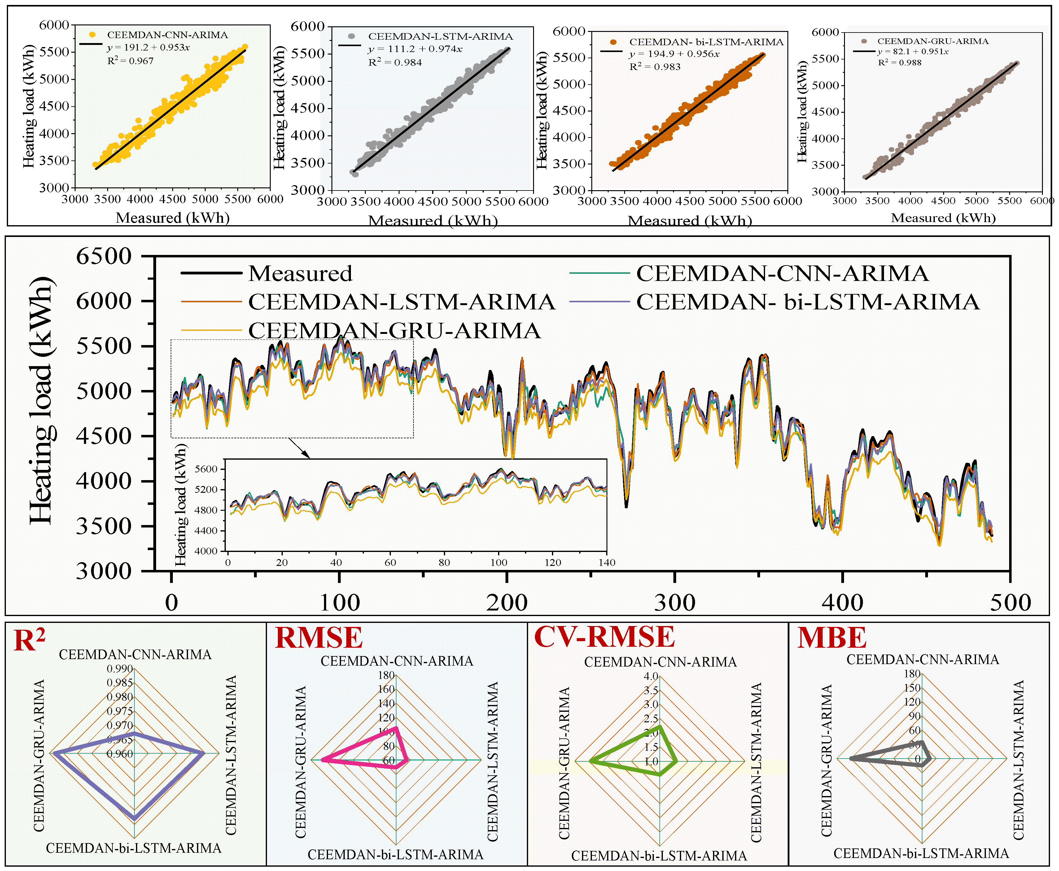
Model prediction: The prediction of the four DL models and the ARIMA model are summed. Thus, the predictions obtained are from four combined models, namely CEEMDAN-CNN-ARIMA, CEEMDAN-LSTM-ARIMA, CEEMDAN-GRU-ARIMA, and CEEMDAN-bi-LSTM-ARIMA.

The adaptive moment estimation (Adam) method is adopted to optimize the weights of the CNN, LSTM, bi-LSTM, and GRU networks. The reader can refer to [45] for an introduction to Adam. The hyper-parameters optimized for the four DL models are shown in

Table 1. Hyper-parameters of DL models for building heating load prediction.

Models	Parameters	Maximum Values	Minimum Values
CNN	Filters	1	30
	Kernels	1	3
	Dropout rate	0.1	0.5
	Pooling size	1	2
	Layers	1	5
	Learning rate	0.01	0.1
	Epochs	10	100
	Batch size	12	72
LSTM	LSTM layers	1	5
	Dense layers	1	3
	LSTM units	10	100
	Dropout rate	0.1	0.5
	Dense units	10	100
	Batch size	12	72
	Epochs	10	100
	Learning rate	0.01	0.1
GRU	GRU layers	1	5
	Dense layer	1	3
	GRU units	10	100
	Dropout rate	0.1	0.5
	Dense units	10	100
	Batch size	12	72
	Epochs	10	100
	Learning rate	0.01	0.1
Bi-LSTM	Bi-LSTM layers	1	5
	Dense layers	1	3
	Dropout rate	0.1	0.5
	Dense units	10	100
	Batch size	12	72
	Epochs	10	100
	Learning rate	0.01	0.1

. In this study, the Tree of Parzen Estimators (TPE) [53] method was used to optimize the hyper parameters, where the number of maximum estimations was set to be 100.

4. Results and Discussion

To verify the performance of the combined models proposed in this study, eight models, namely CNN, LSTM, GRU, bi-LSTM, CEEMDAN-CNN, CEEMDAN-LSTM, CEEMDAN-GRU, and CEEMDAN-bi-LSTM, were implemented and compared.

The CNN, LSTM, GRU, and bi-LSTM are one-step prediction models and were adopted to predict the heating load without any data preprocessing. CEEMDAN-CNN, CEEMDAN-LSTM, CEEMDAN-GRU, and CEEMDAN-bi-LSTM are the two-step prediction models based on the CEEMDAN algorithm, where the components of the heating load, including the IMFs and RES were decomposed using CEEMDAN algorithm and then predicted by the DL models. CEEMDAN-CNN-ARIMA, CEEMDAN-LSTM-ARIMA, CEEMDAN-GRU-ARIMA, and CEEMDAN-bi-LSTM-ARIMA are the three-step prediction models, which combine the DL models, the CEEMDAN algorithm, and the ARIMA model, where the ARIMA model is adopted to predict the components of low frequencies instead of the DL models.

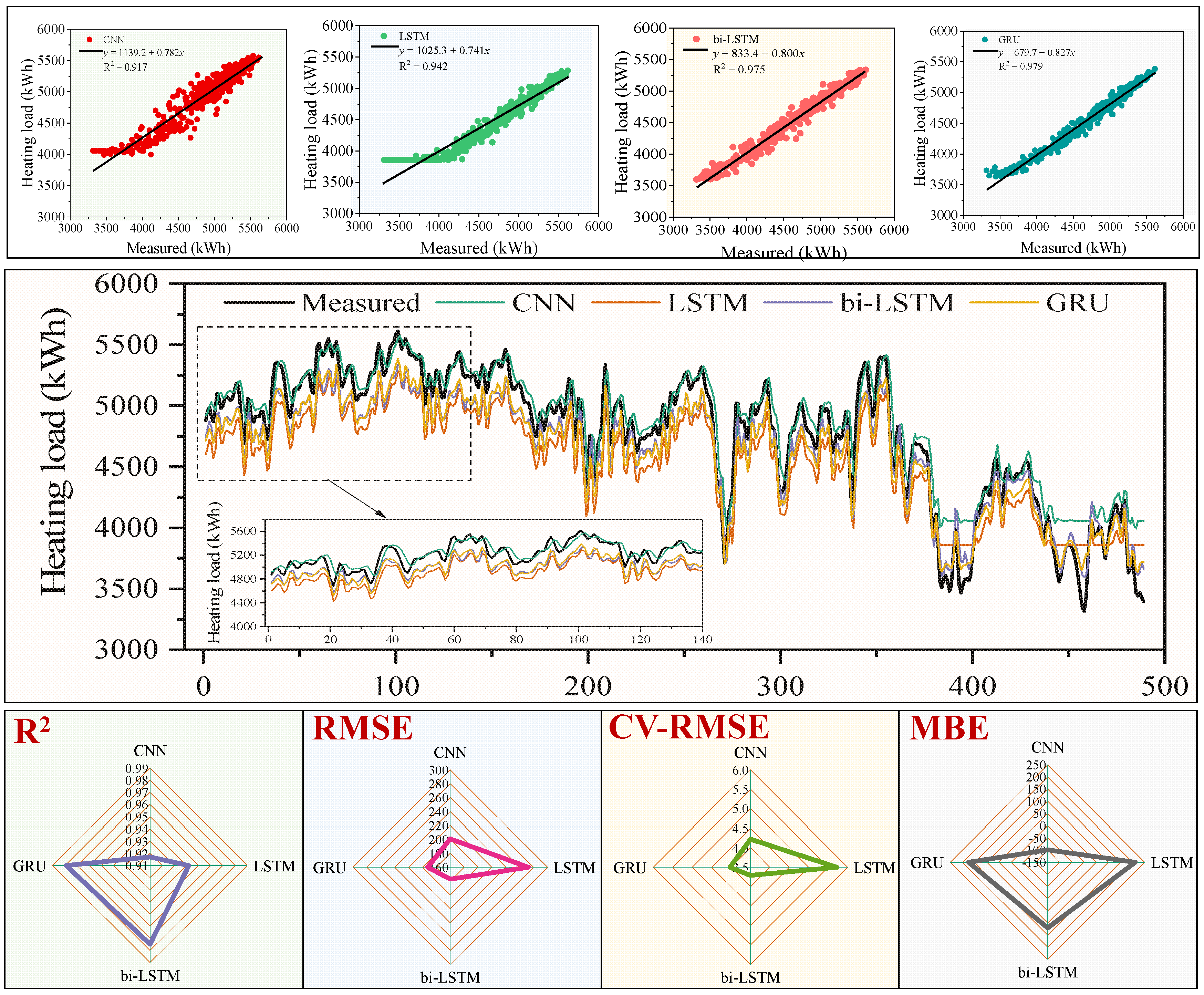
4.1. Model Performance Comparison

Table 2. Evaluation indicators of different models for short-term building heating load prediction.

Models	Model ID	R2	RMSE (kWh)	CV-RMSE (%)	MBE (kWh)
CNN	C1	0.917	200.98	4.22	−99.16
CEEMDAN-CNN	C2	0.967	196.15	4.12	158.74
CEEMDAN-CNN-ARIMA	C3	0.967	104.63	2.20	34.12
LSTM	L1	0.942	272.72	5.72	210.74
CEEMDAN-LSTM	L2	0.981	94.04	1.97	44.13
CEEMDAN-LSTM-ARIMA	L3	0.984	74.53	1.56	16.32
Bi-LSTM	B1	0.975	177.06	3.71	120.60
CEEMDAN- Bi-LSTM	B2	0.983	92.27	1.94	−22.17
CEEMDAN- Bi-LSTM-ARIMA	B3	0.983	70.25	1.47	14.25
GRU	G1	0.979	192.40	4.03	174.81
CEEMDAN-GRU	G2	0.988	182.69	3.83	142.34
CEEMDAN-GRU-ARIMA	G3	0.988	163.00	3.42	149.66

shows the evaluation indicators of the one-, two-, and three-step prediction models. Overall, all models achieved high accuracy. R², RMSE, CV-RMSE, and MBE varied from 0.917–0.988, 70.25–272.72 kWh, 1.47–5.72%, and −99.16–210.74 kWh with average values of 0.971, 151.73 kWh, 3.18%, and 78.70 kWh, respectively.

Figure 9 shows the prediction results of the one-step prediction models. For the CNN model, it can be seen in the diagram of Figure 8 that before the 350th heating load sample, the predicted heating load showed good agreement with the measured values. However, after the 350th sample, the agreement between them gradually deteriorated, which was the cause of the lowest R² values. The main reason is that in the early stage of testing, the heating load change trend is similar to that in the training phases. Thus, the CNN model could fit the training set very well through its multi-layer structure. That is, when the change trend in the test phase is similar to that of the training phase, the CNN models will produce excellent predictions. However, as time progressed, the temperature gradually warmed up, the heating load gradually decreased, and the change trend of the heating load began to change. Because the CNN model does not have any memory, it is difficult to capture the change trend of long-lasting series. As a result, the coincidence of CNN prediction and measured values declined after that point.

Although the change trend of the LSTM model’s heating load prediction was similar to that of the measured values at all stages, its deviation degree was high. Therefore, the R² value of LSTM was higher than that of CNN, while the RMSE and CV-RMSE were higher than those of CNN. Moreover, it can be seen from Figure 8 that the coincidence degree of the LSTM continued to improve as time progressed. This is because the LSTM has a memory function and continues to learn through the prediction, so its performance improves continuously. Similarly, the performance of bi-LSTM and GRU also improved continuously, and the agreement between heating load predictions and measured values was very high in all testing phases.

Comparing the GRU and the bi-LSTM, it can be seen that the GRU had higher R² value, while the bi-LSTM yielded lower RMSE, CV-RMSE, and MBE. Building heating load is related to climate conditions, historical heating loads, building characteristics, and other factors, and its randomness is strong. The bi-LSTM generates the current prediction value considering the past and future information of time series, so its prediction is relatively smooth, resulting in poor consistency of the change trend between the predicted and the measured values compared with the GRU. However, because the bi-LSTM integrates these additional aspects of the time series, its prediction deviation is smaller than that of the GRU, and the prediction error is smaller. Thus, the RMSE, CV-RMSE, and MBE of bi-LSTM were lower than the corresponding values of the GRU.

Figure 10 shows a comparison of predicted and measured heating load of the two-step prediction models, in which it can be easily seen that the performance was greatly improved compared with one-step prediction models. The average R², RMSE, CV-RMSE, and MBE were 0.980, 143.72 kWh, 3.02%, and 88.88 kWh, respectively, improved by 2.78%, 31.03%, 31.01%, and 5.08% compared to the corresponding one-step prediction models. Similarly, CEEMDAN-GRU produced the highest R² at a value of 0.988, while CEEMDAN-bi-LSTM yielded the lowest RMSE and CV-RMSE with values of 92.27 kWh and 1.94%, respectively.

Figure 11 shows a comparison of the predicted and measured heating load of the three-step prediction models. In a similar fashion to the previous comparison, compared with two-step prediction models, the performance was greatly improved, with average R² = 0.981, RMSE = 103.10 kWh, CV-RMSE = 2.16%, and MBE = 55.58 kWh. These values were improved by 0.08%, 28.26%, 28.28%, and 39.71%, respectively. CEEMDAN-CNN-ARIMA had worst performance; the R² value of CEEMDAN-GRU-ARIMA was the highest one; CEEMDAN-bi-LSTM-ARIMA produced the best performance with the lowest RMSE, CV-RMSE, and MBE.

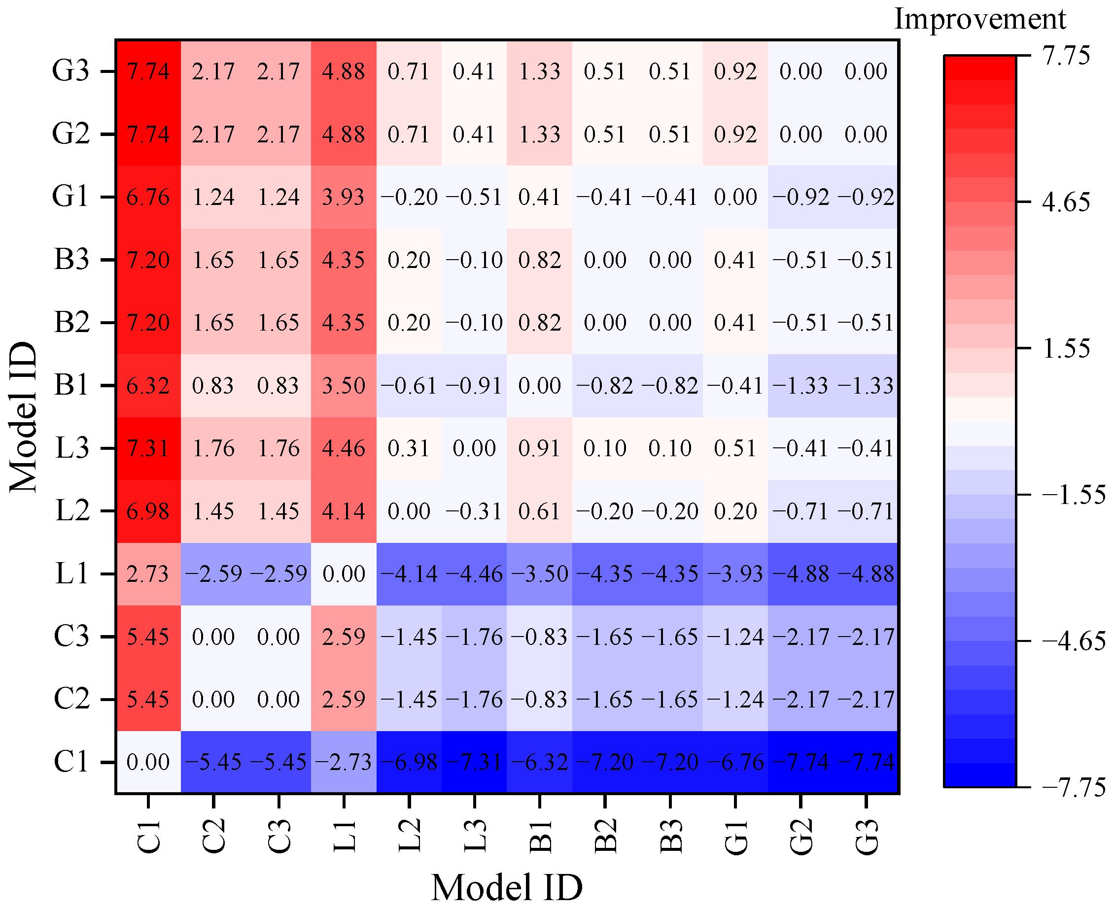
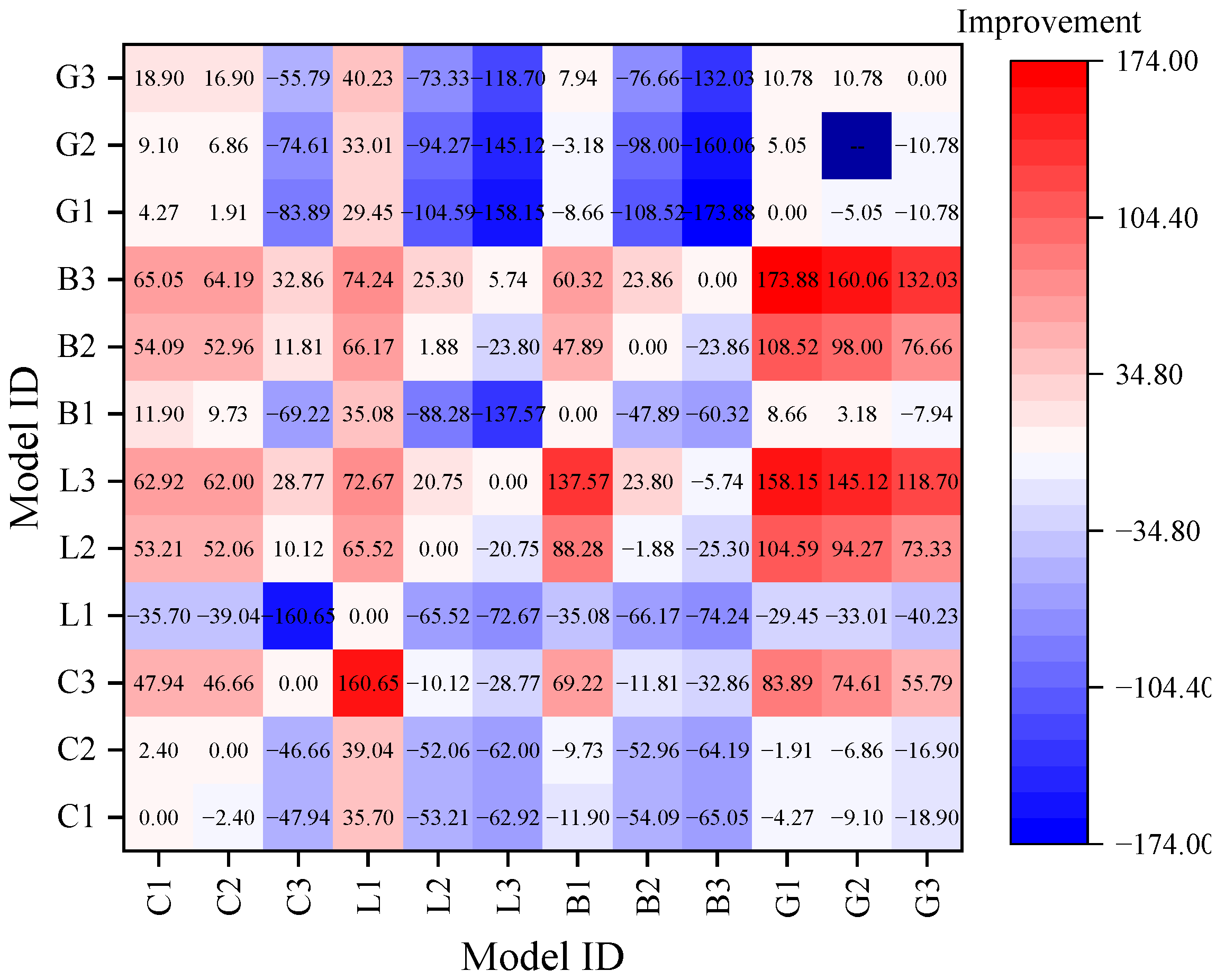
4.2. Improvements of Combined Models

Figure 12, Figure 13 and Figure 14 show the performance improvement percentages of the models investigated in this paper. It is evident that with regard to prediction accuracy, increasing the number of steps generally improved the prediction results. Furthermore, one-step models with worse performance showed higher performance improvement when used in combined models. For example, compared with one-step models, CNN models yielded the lowest R², while GRU models have highest R². The performance improvement percentages of the two- and three-step models were 5.45% and 5.45%, respectively. In contrast, the corresponding values for GRU were 0.92% and 0.92%, respectively.

Compared to one-step models, the performance improvement percentages of R², RMSE, and CV-RMSE of the two-step models were 2.83%, 30.22%, and 30.15%, respectively, and 2.91%, 47.93%, and 47.92% for the three-step models.

5. Conclusions

Accurate prediction of building energy consumption is of great significance to building energy management systems. In this paper, a model combining DL models (including CNN, LSTM, bi-LSTM, GRU) and the ARIMA model is proposed based on CEEMDAN. The CEEMDAN model was used to decompose the original heating load data, while the DL models were used to predict complex high-frequency subsequences; the ARIMA model was used to predict relatively stable low-frequency subsequences. Through the validation of models using actual heating load data, the following conclusions are obtained:

(1)

At the initial stage of testing, the change trend of the heating load is similar to that observed during training phases, and the CNN model could follow the heating load due to its deep structure. Therefore, at the initial stage of testing, the CNN had the best performance. As time progressed, the heating load gradually decreased, the change trend became less familiar to the model, and the CNN prediction performance decreased. In comparison, the LSTM, bi-LSTM, and GRU have memory functions resulting in their prediction performance improving over time. The Bi-LSTM had the best comprehensive performance because it can integrate information from the previous and the following samples of the time series.

(2)

Combined models performed better than single models. Compared with the single model, the average performance improvement percentages of R², RMSE, and CV-RMSE of the two-step models combining CEEMDAN and DL models were 2.83%, 30.22%, and 30.15%, respectively. The corresponding values of the three-step models, which combined CEEMDAN, DL, and ARIMA, were 2.91%, 47.93%, and 47.92%, respectively.

(3)

Among all models, the CEEMDAN-Bi-LSTM-ARIMA model had the best performance. ARIMA model can predict the low-frequency subsequences decomposed by CEEMDAN effectively and reduce the prediction error of the bi-LSTM on these low-frequency subsequences. This resulted in an improvement in the overall prediction accuracy of the hybrid model.

In conclusion, building energy consumption has high-dimensional nonlinearity and randomness. The CEEEMD-DL-ARIMA model can not only solve the problem of BECP but also solve other time series prediction problems, such as the solar radiation prediction problem. However, the different components of the model are still summed using a simple linear weighting. As the time series changes dynamically, the weight of each component also changes dynamically as time progresses. Therefore, in future research, a variable weight combination method should be considered to improve the prediction accuracy of building energy consumption.

References

1. Lu, C.; Li, S.; Lu, Z. Building energy prediction using artificial neural networks: A literature survey. Energy Build. 2022, 262, 111718. [Google Scholar] [CrossRef]
2. Olu-Ajayi, R.; Alaka, H.; Sulaimon, I.; Sunmola, F.; Ajayi, S. Building energy consumption prediction for residential buildings using deep learning and other machine learning techniques. J. Build. Eng. 2022, 45, 103406. [Google Scholar] [CrossRef]
3. Li, A.; Xiao, F.; Zhang, C.; Fan, C. Attention-based interpretable neural network for building cooling load prediction. Appl. Energy 2021, 299, 117238. [Google Scholar] [CrossRef]
4. Razmjooy, N.; Ramezani, M. Uncertain Method for Optimal Control Problems with Uncertainties Using Chebyshev Inclusion Functions. Asian J. Control 2019, 21, 824–831. [Google Scholar] [CrossRef]
5. Razmjooy, N.; Ramezani, M. Interval structure of Runge-Kutta methods for solving optimal control problems with uncertainties. J. Comput. Methods Differ. Equ. 2019, 7, 235–251. [Google Scholar]
6. Jang, Y.; Byon, E.; Jahani, E.; Cetin, K. On the long-term density prediction of peak electricity load with demand side management in buildings. Energy Build. 2020, 228, 110450. [Google Scholar] [CrossRef]
7. Fang, X.; Gong, G.; Li, G.; Chun, L.; Li, W.; Peng, P. A hybrid deep transfer learning strategy for short term cross-building energy prediction. Energy 2021, 215, 119208. [Google Scholar] [CrossRef]
8. Dong, Z.; Liu, J.; Liu, B.; Li, K.; Li, X. Hourly energy consumption prediction of an office building based on ensemble learning and energy consumption pattern classification. Energy Build. 2021, 241, 110929. [Google Scholar] [CrossRef]
9. Liu, Y.; Hu, X.; Luo, X.; Zhou, Y.; Wang, D.; Farah, S. Identifying the most significant input parameters for predicting district heating load using an association rule algorithm. J. Clean. Prod. 2020, 275, 122984. [Google Scholar] [CrossRef]
10. Baglivo, C.; Congedo, P.M.; Murrone, G.; Lezzi, D. Long-term predictive energy analysis of a high-performance building in a mediterranean climate under climate change. Energy 2022, 238, 121641. [Google Scholar] [CrossRef]
11. Gassar, A.A.A.; Cha, S.H. Energy prediction techniques for large-scale buildings towards a sustainable built environment: A review. Energy Build. 2020, 224, 110238. [Google Scholar] [CrossRef]
12. Zhang, Q.; Tian, Z.; Ma, Z.; Li, G.; Lu, Y.; Niu, J. Development of the heating load prediction model for the residential building of district heating based on model calibration. Energy 2020, 205, 117949. [Google Scholar] [CrossRef]
13. Shabunko, V.; Lim, C.M.; Mathew, S. EnergyPlus models for the benchmarking of residential buildings in Brunei Darussalam. Energy Build. 2018, 169, 507–516. [Google Scholar] [CrossRef]
14. Wei, Y.; Zhang, X.; Shi, Y.; Xia, L.; Pan, S.; Wu, J.; Han, M.; Zhao, X. A review of data-driven approaches for prediction and classification of building energy consumption. Renew. Sustain. Energy Rev. 2018, 82, 1027–1047. [Google Scholar] [CrossRef]
15. Sun, Y.; Haghighat, F.; Fung, B.C.M. A review of the-state-of-the-art in data-driven approaches for building energy prediction. Energy Build. 2020, 221, 110022. [Google Scholar] [CrossRef]
16. Zhang, L.; Wen, J.; Li, Y.; Chen, J.; Ye, Y.; Fu, Y.; Livingood, W. A review of machine learning in building load prediction. Appl. Energy 2021, 285, 116452. [Google Scholar] [CrossRef]
17. Elbeltagi, E.; Wefki, H. Predicting energy consumption for residential buildings using ANN through parametric modeling. Energy Rep. 2021, 7, 2534–2545. [Google Scholar] [CrossRef]
18. Ahmad, A.S.; Hassan, M.Y.; Abdullah, M.P.; Rahman, H.A.; Hussin, F.; Abdullah, H.; Saidur, R. A review on applications of ANN and SVM for building electrical energy consumption forecasting. Renew. Sustain. Energy Rev. 2014, 33, 102–109. [Google Scholar] [CrossRef]
19. Chen, B.; Liu, Q.; Chen, H.; Wang, L.; Deng, T.; Zhang, L.; Wu, X. Multiobjective optimization of building energy consumption based on BIM-DB and LSSVM-NSGA-II. J. Clean. Prod. 2021, 294, 126153. [Google Scholar] [CrossRef]
20. Yu, Z.; Haghighat, F.; Fung, B.C.M.; Yoshino, H. A decision tree method for building energy demand modeling. Energy Build. 2010, 42, 1637–1646. [Google Scholar] [CrossRef] [Green Version]
21. Xiao, Z.; Gang, W.; Yuan, J.; Zhang, Y.; Fan, C. Cooling load disaggregation using a NILM method based on random forest for smart buildings. Sustain. Cities Soc. 2021, 74, 103202. [Google Scholar] [CrossRef]
22. Lu, H.; Cheng, F.; Ma, X.; Hu, G. Short-term prediction of building energy consumption employing an improved extreme gradient boosting model: A case study of an intake tower. Energy 2020, 203, 117756. [Google Scholar] [CrossRef]
23. Ling, J.; Dai, N.; Xing, J.; Tong, H. An improved input variable selection method of the data-driven model for building heating load prediction. J. Build. Eng. 2021, 44, 103255. [Google Scholar] [CrossRef]
24. Chen, Y.; Guo, M.; Chen, Z.; Chen, Z.; Ji, Y. Physical energy and data-driven models in building energy prediction: A review. Energy Rep. 2022, 8, 2656–2671. [Google Scholar] [CrossRef]
25. Liu, Y.; Chen, H.; Zhang, L.; Feng, Z. Enhancing building energy efficiency using a random forest model: A hybrid prediction approach. Energy Rep. 2021, 7, 5003–5012. [Google Scholar] [CrossRef]
26. Liu, J.; Zhang, Q.; Dong, Z.; Li, X.; Li, G.; Xie, Y.; Li, K. Quantitative evaluation of the building energy performance based on short-term energy predictions. Energy 2021, 223, 120065. [Google Scholar] [CrossRef]
27. Lei, L.; Chen, W.; Wu, B.; Chen, C.; Liu, W. A building energy consumption prediction model based on rough set theory and deep learning algorithms. Energy Build. 2021, 240, 110886. [Google Scholar] [CrossRef]
28. Zhou, Y.; Liu, Y.; Wang, D.; Liu, X. Comparison of machine-learning models for predicting short-term building heating load using operational parameters. Energy Build. 2021, 253, 111505. [Google Scholar] [CrossRef]
29. Li, X.; Liu, S.; Zhao, L.; Meng, X.; Fang, Y. An integrated building energy performance evaluation method: From parametric modeling to GA-NN based energy consumption prediction modeling. J. Build. Eng. 2022, 45, 103571. [Google Scholar] [CrossRef]
30. Wang, R.; Lu, S.; Feng, W. A novel improved model for building energy consumption prediction based on model integration. Appl. Energy 2020, 262, 114561. [Google Scholar] [CrossRef]
31. Li, G.; Zhao, X.; Fan, C.; Fang, X.; Li, F.; Wu, Y. Assessment of long short-term memory and its modifications for enhanced short-term building energy predictions. J. Build. Eng. 2021, 43, 103182. [Google Scholar] [CrossRef]
32. Li, K.; Tian, J.; Xue, W.; Tan, G. Short-term electricity consumption prediction for buildings using data-driven swarm intelligence based ensemble model. Energy Build. 2021, 231, 110558. [Google Scholar] [CrossRef]
33. Zhang, C.; Li, J.; Zhao, Y.; Li, T.; Chen, Q.; Zhang, X. A hybrid deep learning-based method for short-term building energy load prediction combined with an interpretation process. Energy Build. 2020, 225, 110301. [Google Scholar] [CrossRef]
34. Zhang, Q.; Tian, Z.; Ding, Y.; Lu, Y.; Niu, J. Development and evaluation of cooling load prediction models for a factory workshop. J. Clean. Prod. 2019, 230, 622–633. [Google Scholar] [CrossRef]
35. Gao, B.; Huang, X.; Shi, J.; Tai, Y.; Zhang, J. Hourly forecasting of solar irradiance based on CEEMDAN and multi-strategy CNN-LSTM neural networks. Renew. Energy 2020, 162, 1665–1683. [Google Scholar] [CrossRef]
36. Gao, Y.; Hang, Y.; Yang, M. A cooling load prediction method using improved CEEMDAN and Markov Chains correction. J. Build. Eng. 2021, 42, 103041. [Google Scholar] [CrossRef]
37. Karijadi, I.; Chou, S.-Y. A hybrid RF-LSTM based on CEEMDAN for improving the accuracy of building energy consumption prediction. Energy Build. 2022, 259, 111908. [Google Scholar] [CrossRef]
38. Zhou, Y.; Liu, Y.; Wang, D.; Liu, X.; Wang, Y. A review on global solar radiation prediction with machine learning models in a comprehensive perspective. Energy Convers. Manag. 2021, 235, 113960. [Google Scholar] [CrossRef]
39. Huang, N.E.; Shen, Z.; Long, S.R.; Wu, M.C.; Shih, H.H.; Zheng, Q.; Yen, N.-C.; Tung, C.C.; Liu, H.H. The empirical mode decomposition and the Hilbert spectrum for nonlinear and non-stationary time series analysis. Proc. R. Soc. Lond. Ser. A Math. Phys. Eng. Sci. 1998, 454, 903–995. [Google Scholar] [CrossRef]
40. Wu, Z.; Huang, N.E. Ensemble empirical mode decomposition: A noise-assisted data analysis method. Adv. Adapt. Data Anal. 2009, 1, 1–41. [Google Scholar] [CrossRef]
41. Torres, M.E.; Colominas, M.A.; Schlotthauer, G.; Flandrin, P. A complete ensemble empirical mode decomposition with adaptive noise. In Proceedings of the 2011 IEEE International Conference on Acoustics, Speech and Signal Processing (ICASSP), Prague, Czech Republic, 22–27 May 2011; pp. 4144–4147. [Google Scholar]
42. Song, J.; Zhang, L.; Xue, G.; Ma, Y.; Gao, S.; Jiang, Q. Predicting hourly heating load in a district heating system based on a hybrid CNN-LSTM model. Energy Build. 2021, 243, 110998. [Google Scholar] [CrossRef]
43. Kumari, P.; Toshniwal, D. Long short term memory–convolutional neural network based deep hybrid approach for solar irradiance forecasting. Appl. Energy 2021, 295, 117061. [Google Scholar] [CrossRef]
44. Li, X.; Chen, Q. Development of a novel method to detect clothing level and facial skin temperature for controlling HVAC systems. Energy Build. 2021, 239, 110859. [Google Scholar] [CrossRef]
45. Liu, M.-D.; Ding, L.; Bai, Y.-L. Application of hybrid model based on empirical mode decomposition, novel recurrent neural networks and the ARIMA to wind speed prediction. Energy Convers. Manag. 2021, 233, 113917. [Google Scholar] [CrossRef]
46. Yu, C.; Li, Y.; Bao, Y.; Tang, H.; Zhai, G. A novel framework for wind speed prediction based on recurrent neural networks and support vector machine. Energy Convers. Manag. 2018, 178, 137–145. [Google Scholar] [CrossRef]
47. Yan, X.; Guan, T.; Fan, K.; Sun, Q. Novel double layer BiLSTM minor soft fault detection for sensors in air-conditioning system with KPCA reducing dimensions. J. Build. Eng. 2021, 44, 102950. [Google Scholar] [CrossRef]
48. Khashei, M.; Bijari, M. A novel hybridization of artificial neural networks and ARIMA models for time series forecasting. Appl. Soft Comput. 2011, 11, 2664–2675. [Google Scholar] [CrossRef]
49. Liu, Y.; Zhou, Y.; Wang, D.; Wang, Y.; Li, Y.; Zhu, Y. Classification of solar radiation zones and general models for estimating the daily global solar radiation on horizontal surfaces in China. Energy Convers. Manag. 2017, 154, 168–179. [Google Scholar] [CrossRef]
50. Zhou, Y.; Liu, Y.; Wang, D.; De, G.; Li, Y.; Liu, X.; Wang, Y. A novel combined multi-task learning and Gaussian process regression model for the prediction of multi-timescale and multi-component of solar radiation. J. Clean. Prod. 2021, 284, 124710. [Google Scholar] [CrossRef]
51. Jia, S.; Ma, B.; Guo, W.; Li, Z.S. A sample entropy based prognostics method for lithium-ion batteries using relevance vector machine. J. Manuf. Syst. 2021, 61, 773–781. [Google Scholar] [CrossRef]
52. Ma, Z.; Chen, H.; Wang, J.; Yang, X.; Yan, R.; Jia, J.; Xu, W. Application of hybrid model based on double decomposition, error correction and deep learning in short-term wind speed prediction. Energy Convers. Manag. 2020, 205, 112345. [Google Scholar] [CrossRef]
53. Bergstra, J.; Yamins, D.; Cox, D.D. Making a Science of Model Search: Hyperparameter Optimization in Hundreds of Dimensions for Vision Architectures. In Proceedings of the International Conference on Machine Learning, Atlanta, GA, USA, 16–21 June 2013; pp. 115–123. [Google Scholar]
Figure 1. Combined model structure for building heating load prediction.
Sustainability 14 07349 g001
Figure 2. General topological structure of a CNN model.
Sustainability 14 07349 g002
Figure 3. General topological structure of LSTM model.
Sustainability 14 07349 g003
Figure 4. General topological structure of GRU model.
Sustainability 14 07349 g004
Figure 5. General topological structure of Bi-LSTM.
Sustainability 14 07349 g005
Figure 6. Heating load and the corresponding intrinsic mode functions and residuals decomposed using CEEMDAN.
Sustainability 14 07349 g006
Figure 7. Correlation analysis between current heating load and historical heating loads.
Sustainability 14 07349 g007
Figure 8. Sample entropy of the components decomposed using CEEMDAN.
Sustainability 14 07349 g008
Figure 9. Comparison of prediction results of one-step prediction models.
Sustainability 14 07349 g009
Figure 10. Comparison of prediction results of two-step prediction models.
Sustainability 14 07349 g010
Figure 11. Comparison of prediction results of three-step prediction models.
Sustainability 14 07349 g011
Figure 12. Improvement percentage of R2 between different models investigated in this study. Notes: Improvement of R2 = (R2 in columns − R2 in rows)/R2 in columns.
Sustainability 14 07349 g012
Figure 13. Improvement percentage of RMSE between different models investigated in this study (%). Notes: Improvement of RMSE = (RMSE in columns − RMSE in rows)/RMSE in columns.
Sustainability 14 07349 g013
Figure 14. Improvement percentage of RMSE between different models investigated in this study (%). Notes: Improvement of CV-RMSE = (CV-RMSE in columns − CV-RMSE in rows)/CV-RMSE in columns.
Sustainability 14 07349 g014