Does the Inclusion of Spatio-Temporal Features Improve Bus Travel Time Predictions? A Deep Learning-Based Modelling Approach

Abstract

With the abundance of public transportation in highly urbanized areas, it is common for passengers to make inefficient or flawed transport decisions due to a lack of information. The exact arrival time of a bus is an example of such information that can aid passengers in making better decisions. The purpose of this study is to provide a method for predicting path-based bus travel time, thereby assisting accurate bus arrival and departure time predictions at each bus stop. Specifically, we develop a Geo-conv Long Short-term Memory (LSTM) model that (1) extracts subsequent spatial features through a 1D Convolution Neural Network (CNN) for the entire bus travel sequence and (2) captures the temporal dependencies between subsequences through the LSTM network. Additionally, this study utilizes additional variables that affect two components of bus travel time (dwelling time and transit time) to precisely predict travel time. The constructed model is then evaluated by the practical application to two bus lines operating in Seoul, Korea. The results show that our model outperforms three other baseline models. Two bus lines with different types of operation show different model performance patterns that are dependent on travel distance. Interestingly, we find that the variable related to the link of the stop location appears to play an important role in predicting bus travel time. We believe that these novel findings will contribute to the literature on transportation and, in particular, on deep learning-based travel time prediction.

1. Introduction

About 55 percent of the world’s population lives in urban areas, and this proportion is projected to reach 68 percent by 2050 [1]. Urbanization, a process in which the population moves from a rural area to an urban area, is accelerating, which apparently causes various social problems. In particular, as the population density in urban areas increases, traffic congestion is likely to worsen, resulting in enormous social costs. The transportation sector is a major source of greenhouse gas emissions that experiences strong growth from the road sector, accounting for 14% of global greenhouse gas emissions on average over the past decade [2]. In order to reduce greenhouse gas emissions in the transportation field, the excessive use of private cars and automobile dependency need to diminish. Thus, the use of public transportation, which is commonly known as being an eco-friendly or less-motorized mode of transportation, should be promoted in the context of sustainability.

As a practical way to encourage the use of public transit, policies are being implemented to improve user convenience, including real-time bus arrival information systems and integrated public transit fare systems with conditional free transfers. With the development of Information and Communications Technology, the real-time GPS coordinates of buses are legally collected by public transportation authorities, which allows users to know the bus arrival time via their smartphones, even if they are unfamiliar with bus routes. Accordingly, they can obtain information about the location of the available buses in operation and when the first one will arrive, thereby reducing the time spent waiting for the bus at a stop. Bus travel time information not only helps users make decisions but also plays an important role in public transportation operations. Public transportation operators want to provide maximum service to passengers with the minimum amount of resource input. Therefore, it is necessary to design an optimal public transportation network that can be divided into five stages: line design, frequency setting, timetable development, bus scheduling, and driver scheduling [3]. Bus travel time information is regarded as an essential decision-making variable in the optimization process during the line design [4,5,6,7,8,9] and frequency setting [4,8] stages. It is also used to evaluate the performance of bus routes [10,11,12], and routes are evaluated by quantifying the reliability of bus operation, which is mainly based on variance in the bus travel time. In addition to the five steps proposed by Cedar and Wilson [3], bus travel time information is also used to solve fleet assignment problems [13]. Finally, it allows public transportation authorities to plan timetables (e.g., determining how often buses should be operated given the traffic condition based on real-time bus operation information).

However, for the above to be effective, how to accurately predict bus travel times after taking road traffic conditions into account should be prioritized.

The traffic flow conditions on complex roads in urban areas are affected by many external factors. For example, conflicts such as traffic congestion occur due to various means of transportation operating simultaneously on a limited road space. Additionally, the introduction of new means of transportation such as personal modes of transportation (electric scooters, Segways, etc.) can also influence traffic flow. Moreover, the construction of eco-friendly bicycle paths through ‘road diets’ can cause a decrease in the overall road capacity for automobiles. In some cities, efforts have been made to improve the pedestrian environment by providing sufficient space for pedestrians, and the interval distance of crosswalks tends to be shorter. This means that accurately predicting bus travel times becomes increasingly difficult because there are a myriad of external factors affecting road speed.

Bus travel time predictions can be accomplished by two approaches. The first method is to predict the travel time of the entire trip by accumulating the travel time between bus stops. The other method is to predict the travel time from a given departure stop to an arrival stop as a path without dividing the travel into segments (i.e., a path-based approach). However, the former has a limitation: travel time errors can be accumulated during the calculations for each. When calculated via the latter method, the predicted bus travel time can be used to calculate the required time when public transportation users plan a bus trip in advance. Based on that information, potential passengers can determine the departure time and bus route. Nevertheless, a limitation of the current system is that it only provides the average travel time as calculated based on past bus travel records.

Given the background information above, this study aims to predict the path-based bus travel time for a given departure and arrival bus stop. In previous studies, bus travel time was predicted using historical methods, statistical models, and machine learning methods using the GPS coordinates collected from the bus. In this study, however, spatio-temporal features are incorporated to accurately predict bus travel time using a deep learning-based model. Furthermore, the number of passengers boarding (or alighting from) a bus and the road speed are taken into account since bus travel time consists of a link travel time and dwelling time. The contributions of this paper are summarized as follows:

• Model Structure: In this study, we attempt to develop a bus travel time prediction model by considering spatiotemporal features by combining CNN and LSTM. The CNN layer captures the spatial features by extracting the relationship between adjacent bus stops in the bus stop sequence. Then, the temporal features of the bus travel time are captured through the LSTM layer.
• Input features: We take a wide variety of variables that can affect bus travel into account. In addition to bus stop-specific features, road speed features at the time when the bus is running, vehicle driver features, and weather features are used.
• We evaluate our proposed model through a dataset comprising two real-world bus lines. The experimental results show that the proposed model is superior to other baseline models.

The structure of this paper is as follows: In the next section, previous studies related to bus travel time predictions are reviewed to identify the pros and cons of their method. The following section defines the problem and provides a detailed description of the prospective architecture of the model, including the network topology and dataset preparation. In Section 4, the estimated model is evaluated by focusing on two bus routes in Seoul and is then compared to baseline models. Lastly, our key findings and contributions are summarized followed by an outline of the limitations and future directions of our research.

2. Related Work

A variety of travel time prediction methods have been developed in past decades. These methods can be categorized into three categories: naive, theoretical, and data-driven models [14].

First, naive models have the advantage of being simple and fast as they can predict the travel time without having to undergo learning or parameter estimation. In this respect, it is mainly used for the purposes of providing commercial information and is used as a baseline model for comparison in the literature. For example, a historical method predicts travel time through historical data, which assumes that at certain times, traffic conditions are similar to those at the same time in the past [15,16,17]. Chung and Shalaby [16] proposed a bus arrival time prediction model that calculated the travel time based on past travel times and the current operational conditions. Schedule adherence and weather conditions were considered as operational conditions, and the average travel times for the five days before the target day were also selected. However, the model has a disadvantage: it relied on the statistical average of past traffic hours, which do not reflect changes in traffic time resulting from intermittent external effects (e.g., traffic accidents) [18]. Second, there are models based on traffic theory. These models predict travel time using simulations that recreate scenarios based on various parameters that represent traffic conditions such as density, flow, and speed. However, it is difficult to accurately recreate how the road conditions are affected by various factors in reality with only a few variables [14]. Third, data-driven approaches find a mapping function that calculates the travel time from a large amount of historical data [19,20]. Depending on what specific distribution assumptions are applied to the data, they can be classified into parametric and non-parametric models.

The most representative parametric model is linear regression [21,22,23,24,25,26], which is based on the linear relationships between independent and dependent variables. Current and past traffic condition variables were incorporated as independent variables [21,22,23], and tests including other possible variables such as the departure time, day, and day of week indicates the travel context [21]. In particular, bus travel time predictions have been conducted using multi-linear regression models to combine various independent variables (e.g., length of links, number of passengers, number of stops or intersections, arrival time between stops, geographical factors, etc.) [24,25,26]. However, the model’s predicted influence on travel time was different depending on the combination of independent variables, and the accuracy was low where there was high congestion. Those drawbacks limit its possibility of being a conventional model [27,28]. Another parametric model is the time-series model. The Kalman filter model is a recursive estimation algorithm that continuously updates the travel time state variable through new observations. It has the advantage of easy data preparation. However, the prediction accuracy depends on the state transition model, and it deals with the rapid changes in the travel time at each time-lag with difficulty [29]. Additionally, since a linear filter is usually used in the Kalman filter (KF) model, it was difficult to capture non-linear dynamic features. To overcome this, an extended KF model allowing non-linearity has been proposed, but when the results were produced simultaneously for multiple links, the computational costs rapidly increased [18]. The Autoregressive Integrated Moving Average (ARIMA) model is also a time-series models. Early research predicted travel time using a general univariate ARIMA model [30], and efforts have been made to modify models to improve their prediction accuracy, such as the seasonal ARIMA (SARIMA) model, which was modified according to seasonal differences [31] and combines the SARIMA and KF [32] and the multivariate ARIMA model [33].

Unlike parametric models, non-parametric models do not assume a specific data distribution. Since the model parameters are determined by the collected data and not a predetermined distribution, they require a larger amount of data than many other approaches [34]. Non-parametric methods include Support Vector Regression (SVR) [35,36,37,38], the Nearest Neighborhood model [39,40], and deep-learning based models [18,27,34,41,42,43,44,45,46,47,48,49,50,51,52,53,54,55,56,57,58,59]. In the following subsection, different deep learning-based models are reviewed.

Table 1. Overview of travel time prediction research using deep learning methods.

Research	Target	Experimental Data	Deep Learning Model	External Factors
[41]	Link TT 1	Probe-based travel time	CNN, LSTM	-
[42]	Link TT	Taxi trajectories	LSTM	-
[43]	Route TT	Taxi trajectories	LSTM	-
[27]	TT between bus stops	AVL	LSTM	-
[34]	TT between bus stops	AVL	LSTM	Weather, intersections
[44]	Link TT	Vehicle passage records	CNN + LSTM	-
[45]	Route TT	Taxi trajectories	MLP + LSTM	Weather, driver rider vehicle Profile, traffic restriction
[46]	Route TT	Taxi trajectories	CNN + LSTM	Weather, driver profile
[47,48]	Route TT	Taxi trajectories	CNN + LSTM	-
[51]	Route TT	Vehicle passage records	Graph attention + CNN	-
[52]	Route TT	Taxi trajectories	GCN + CNN	-
[53]	Link speed distribution	Loop detector (highway network) Taxi trajectories (city road network)	GNN	-
[54]	Link travel time distribution parameter	Intersection camera data	GAN (generator: GCN + LSTM, discriminator: MLP)	-
[55]	Route TT	Taxi trajectories	SDNE + CNN + LSTM	Driver profile
[56]	Route TT	Taxi trajectories	GCN + LSTM	-
[18]	TT between bus stops	AVL	CNN + LSTM	-
[57]	TT between bus stops	AVL	LSTM + ANN	-
[58]	Link TT	Taxi trajectories	Denoising auto-encoder	Road segment, contextual features
[59]	TT between bus stops	AVL	DBN	-

¹ TT means travel time.

provides a comprehensive review of the studies predicting the travel time using deep learning models. Deep learning models approach problems through the learning of a very large amount of data, so the GPS trajectories of vehicles with a relatively huge number of data were used to predict travel time [18,27,34,42,43,45,46,47,48,49,50,51,52,53,54,55,56,57,58,59]. Additionally, since trajectory data contains vehicle location information in chronological order, specialized long short-term memory (LSTM) models for sequence-based classification or for solving regression problems have been widely used [18,27,34,41,42,43,44,45,46,47,48,49,50,51,52,53,54,55,56,57].

In early travel time prediction studies using a deep learning model, LSTM models were mainly used [27,34,41,42,43]. Hou and Edara [41] and Lin and Jiang [42] predicted the link travel time using an LSTM model. Hou and Edara [41] showed that the LSTM model outperformed the convolution neural network (CNN) model. Zhang et al. [43] predicted the travel time of the whole path by partitioning the city into grids instead of using raw GPS coordinates (i.e., replacing the GPS coordinate trajectories with grid sequences). Then, using the LSTM layer, the speed features were extracted based on the short-term road speed from one hour before and the long-term road speed from one week before. Based on the grid sequence, even the previous grid features were taken into account for predicting the travel time. Agafonov and Yumaganov [27] and Osama et al. [34] predicted the travel time between bus stops using Automatic Vehicle Location (AVL) data. Agafonov ad Yumaganov [27] used various statistical travel time values such as the average travel time on the same route, the average travel time on different routes, and the average travel time of the bus running immediately before. As a result of the model experiment, it was found that the longer the travel time, the lower the mean absolute percentage error (MAPE) (and the higher the accuracy). Osama et al. [34] used multi-layer perceptron (MLP) and LSTM to predict the bus travel time, respectively. They showed that LSTM performance was superior. In addition, weather and the number of intersections were included as external factors in the model.

Furthermore, the travel time was predicted by combining a layer that reflected the spatial features with the LSTM [18,44,45,46,47,48,49,50,51,52,53,54,55,56,57]. Wei et al. [44] focused on the time-shifting characteristics of urban roads, thereby extracting spatial relationships via Kullback–Leibler divergence and road networks. Then, CNNs and LSTM-based deep neural networks were used to predict the short-term travel speed. Wang and Fu [45] extracted various vehicle path characteristics, using them to predict travel time by applying a deep learning suitable for the attributes of the variables. For example, MLP was applied to numerical variables, embeddings were applied to categorical variables, and LSTM was applied to road segment sequences.

There are many studies that have combined CNNs and LSTM in order to consider spatial features more directly. The research combining CNNs and LSTM can be divided into two categories. First, the travel time was predicted by extracting the sequence characteristics of the trajectories without any modifications [46,47]. Second, the travel time was predicted by reconstructing the trajectory sequence as a road link sequence [48].

Wang et al. [46] divided the entire path of a vehicle into sub-paths via a convolution layer to capture the spatial features between the GPS coordinates and predicted the travel time by extracting the temporal dependence of the sub-paths using the LSTM layer. Additionally, external factors including driver identification variables, weather factors, and the day of the week were selected as variables. Xu et al. [47] developed a model proposed by Wang et al. [46] according to two aspects. First, while Wang et al. [46] did not modify the trajectories, the authors performed embedding so that the road network structure could be reflected in the trajectories. In addition, the road type features were reflected by adding a road type component in terms of the structure of the model. As a result, the mean absolute percentage error (MAPE) decreased by 3%, demonstrating that the accuracy was improved.

Li et al. [48] (1) converted trajectories into the link sequences of road networks, (2) constructed a travel time matrix between links, and (3) extracted spatial features to predict travel times.

A Graph Neural Network (GNN), which is similar to a CNN, was also adopted to capture the spatial features. In particular, GNNs have recently been in the spotlight in the transportation field in that they can represent transportation networks in a graph structure [49,50].

GNN is also used in travel time predictions [51,52,53,54,55]. Fang et al. [51] proposed a Contextual Spatial-Temporal Graph Attention Network (ConSTGAT) that predicts travel time based on a given route and its departure time. ConSTGAT can be divided into two modules. The first “Traffic Prediction” module predicts the traffic conditions by constructing a graph attention network that can simultaneously handle the spatial and temporal information of traffic conditions. Additionally, in the “Contextual Information” module, the relationship between the links constituting the route was extracted through the convolution operation. By integrating the results of these two modules, the travel time of a given route is predicted. Hong et al. [52] combined a GNN and CNN to reflect the temporal correlations through the CNN and the spatial correlations via the GNN. Additionally, three components were composed of recent periods, daily periods, and weekly periods. Hu et al. [53] and Shao et al. [54] tried to predict the speed or time distributions of a road link by focusing on the sparsity of road link information. Hu et al. [53] predicted speed distribution according to the time interval of the road link. To reflect the relationship between road links, the road network structure was encoded using GCN, and information was compressed through a pooling layer. After that, the speed distribution of the link with missing properties was predicted through the decoding process. Similarly, Shao et al. [54] tried to estimate this parameter under the assumption that the travel time of a road link has a normal distribution. A generative adversarial network (GAN) was used; among the GAN components, the generator component generates a normal distribution parameter, and the discriminator component compares it to the real value. At this time, a model combining GCN and LSTM was constructed in the generator component to generate parameters considering spatio-temporal characteristics. Shen et al. [55] proposed a more complex model that incorporated travel speed features, road network structure features, and deep LSTM prediction layers. It is notable that the model uses the tensor deposition method to restore the road speed values that are missing from the grid. Furthermore, structural deep neural embedding (SDNE)—a graph embedding method—was used to extract road network structure features. Based on these grid speed features and road network structure learning results, the travel time was finally predicted using the bi-LSTM layer.

Jin et al. [56] proposed a model for learning each spatial-temporal feature by using node and road segments as edges to reflect the characteristics resulting from the road network structure.

Petersen et al. [18] and Liu et al. [57] predicted the bus travel time by combining LSTM and other artificial neural networks, all of which predicted the travel time between bus stops using AVL data. Petersen et al. [18] proposed a multi-output, multi-time-step deep neural network by combining the convolutional layer and the LSTM layer. The proposed model predicted the travel time for a set time-step using encoder and decoder layers for multiple sections between bus stops. Liu et al. [57] added an artificial neural network (ANN) with one hidden layer to the LSTM. In LSTM, the variation in travel time between bus stops over time was considered, whereas the ANN captured the spatial features via the speed of the bus route link.

Additionally, Tang et al. [58] focused on incorporating contextual city information rather than the structure of deep learning models. A sparse denoising auto-encoder model was employed, and the contextual information included the number of schools, the number of offices, the number of shopping places, etc. Chen et al. [59] also suggested a deep belief network (DBN) that improved the Gaussian–Bernoulli restricted Boltzmann machine when the travel time was continuous. They applied it to predict the travel time between bus stops.

Comprehensively synthesizing the prior results, we can confirm that travel time predictions have been made via the use of deep learning models (thanks to the development of hardware and the collection of big data). In particular, LSTM-based models have been widely used; more recently, there have been scientific efforts to combine various layers that are capable of capturing spatial features with the LSTM layer. These studies can be classified according to whether or not the GPS trajectories were processed. It is noteworthy that when spatial characteristics are extracted by aggregating trajectories in grid units or link units, there is a possibility that the results may be derived differently depending on the size of the grid. Therefore, in this study, we intend to apply the model that predicted the travel time through the LSTM layer proposed by Wang et al. [46] to predict bus travel time in Seoul.

Moreover, we concluded that the consideration of external factors such as weather that can affect travel time was insufficient given the previous findings. In particular, some studies for predicting for the travel times of private cars revealed external factors, but studies for predicting bus travel time did not consider external factors. In the case of bus travel time, the characteristics of each bus stop, such as the number of passengers boarding and alighting at the bus stop and the speed of the road link on which the bus operates, vary depending on location, so we believe that it is imperative to consider these variables. Therefore, we incorporated the bus stop and road link characteristics as well as other factors like the weather, driver, and day of the week.

3. Methods

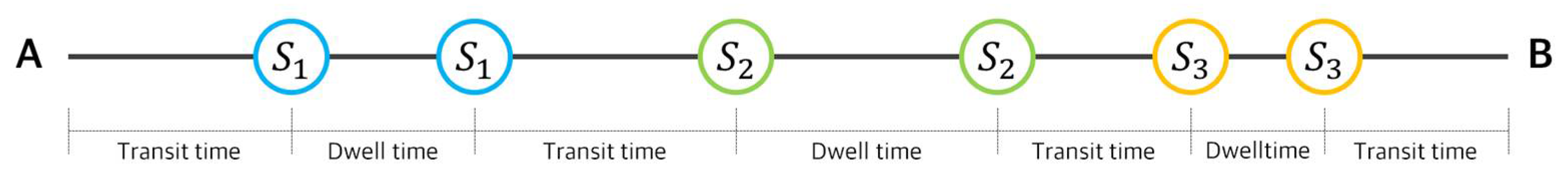
3.1. Problem Definition

The purpose of the model presented in this study is to predict the travel time between two bus stops ($S_a$ and $S_b$). The travel time of a bus is composed of the bus’s actual travel time (transit time) and the time required for passengers to board or alight the bus at the bus stop (dwelling time), as shown in Figure 1. Therefore, in this study, the spatial features of bus stops are captured through bus trajectories. In addition, the factors affecting dwelling time not only take the number of passengers boarding or alighting the bus at each bus stop into account, but also take the number of passengers on the bus and the number of passengers boarding or alighting other routes into account. Finally, we consider the road speed, which affects the transit time of the bus.

Historical Trajectory

The trajectories of the bus from bus stop $i$ to bus stop $j$ were defined as $S=\left\{s_i,\cdots ,s_j\right\}$, $s_i=\{s_{i.lat},s_{i.lng},s_{i.boarding},s_{i.alighting},s_{i.passenger},s_{i.otherBoarding},s_{i.otherAlighting},s_{i.speed},s_{i.lanes},$$s_{i.temp},s_{i.preci}\}$. The information for each stop includes latitude and longitude, the number of passengers boarding or alighting the target bus, the number of passengers on the target bus, the number of passengers boarding or alighting buses other than the target bus, the road speed, the number of road lanes, temperature, and the amount of precipitation where stop $i$ is located. Furthermore, in order to take more externalities into consideration, carID—a feature of the bus driver–the timeslotID, which indicates the time when the bus is running, and weekday factors were added.

Table 2. The glossary of terms.

Notation			Description
$S$			Set of stops
Station	$s_i$		Stop $i$
	Geo-graphical features	$s_{i.lat}$	The latitude of stop $i$
		$s_{i.lng}$	The longitude of stop $i$
	Passenger features	$s_{i.boarding}$	The number of passengers getting on the target bus at the stop $i$
		$s_{i.alighting}$	The number of passengers getting off the target bus at the stop $i$
		$s_{i.passenger}$	The number of passengers on board when the target bus arrives at the stop $i$
		$s_{i.otherBoarding}$	The number of passengers getting on buses other than the target bus at bus stop $i$
		$s_{i.otherAlighting}$	The number of passengers getting off buses other than the target bus at bus stop $i$
	Link features	$s_{i.speed}$	The speed of the link to which the stop $i$ belongs
		$s_{i.lanes}$	The number of lanes of the link to which the stop $i$ belongs
	Weather features	$s_{i.temp}$	Temperature around the stop $i$
		$s_{i.preci}$	Precipitation around the stop $i$
Path	carID		Identity of the vehicle
	timeID		The time slot of the day (1 min: 1)
	weekday		The day of week

represents the notation and their definition. The model learns how to predict the bus travel time based on the spatio-temporal features and the externalities of the stops in the historical trajectory for a given trip afterward.

3.2. Model Architecture

In this section, we describe the architecture of the bus travel time prediction model. As shown in Figure 2, the model incorporates three specific modules: the attribute, spatio-temporal, and prediction modules. The attribute module processes the features of the entire route as external factors, such as the vehicle number of the bus (carID), the bus start time (timeID), and the day of the week (weekday). Its output becomes a partial input of the next module. Then, the spatio-temporal module–the main part of the model–handles both the spatial features of the bus stop sequence and the temporal dependence of the sequence. Using these outcomes, the prediction module subsequently predicts the bus travel time.

3.2.1. Attribute Module

The bus travel time is affected by various external factors. During peak hours, for example, traffic volumes substantially increase, resulting in congested roads. Likewise, transit users usually spend more time boarding and alighting during peak time periods due to crowdedness and waiting passengers. That is, there is a discrepancy between two time periods when a bus runs on the same route: the travel time is longer during peak hours and shorter during off-peak hours. Not surprisingly, this time-dependent feature shows different patterns depending on the day of the week, and driver behavior could lead to different travel times on the same route. Therefore, we incorporated carID, timeID, and weekday as external factors in the attribute module. The timeID is the time at which the vehicle starts operating: one day is divided into 1440 time slots to account for each minute (1 day = 1440 min). It should be noted that the three factors are categorical variables that cannot feed the model directly. This motivates us to use the embedding method to transform a categorical variable into a low-dimensional vector. The embedding method maps the value $v\in \left[V\right]$ of each category to a real space $R^{E\times 1}$. $V$ and $E$ represent the number of categories and the dimensions of the embedding space, respectively. The complexity of the computation can be reduced by decreasing the input dimension according to the embedding method.

Furthermore, we added the travel distance to the output of the attribute module. The total travel distance from stop $a$ to stop $b$ can be represented as $d_{s_a\to s_b}={\displaystyle \sum }_{i=a}^{b-1}D\left(s_i,s_{i+1}\right)$, where $D\left(s_i,s_{i+1}\right)$ is the link-based distance between two adjacent stops. We define the output of attribute module as attr.

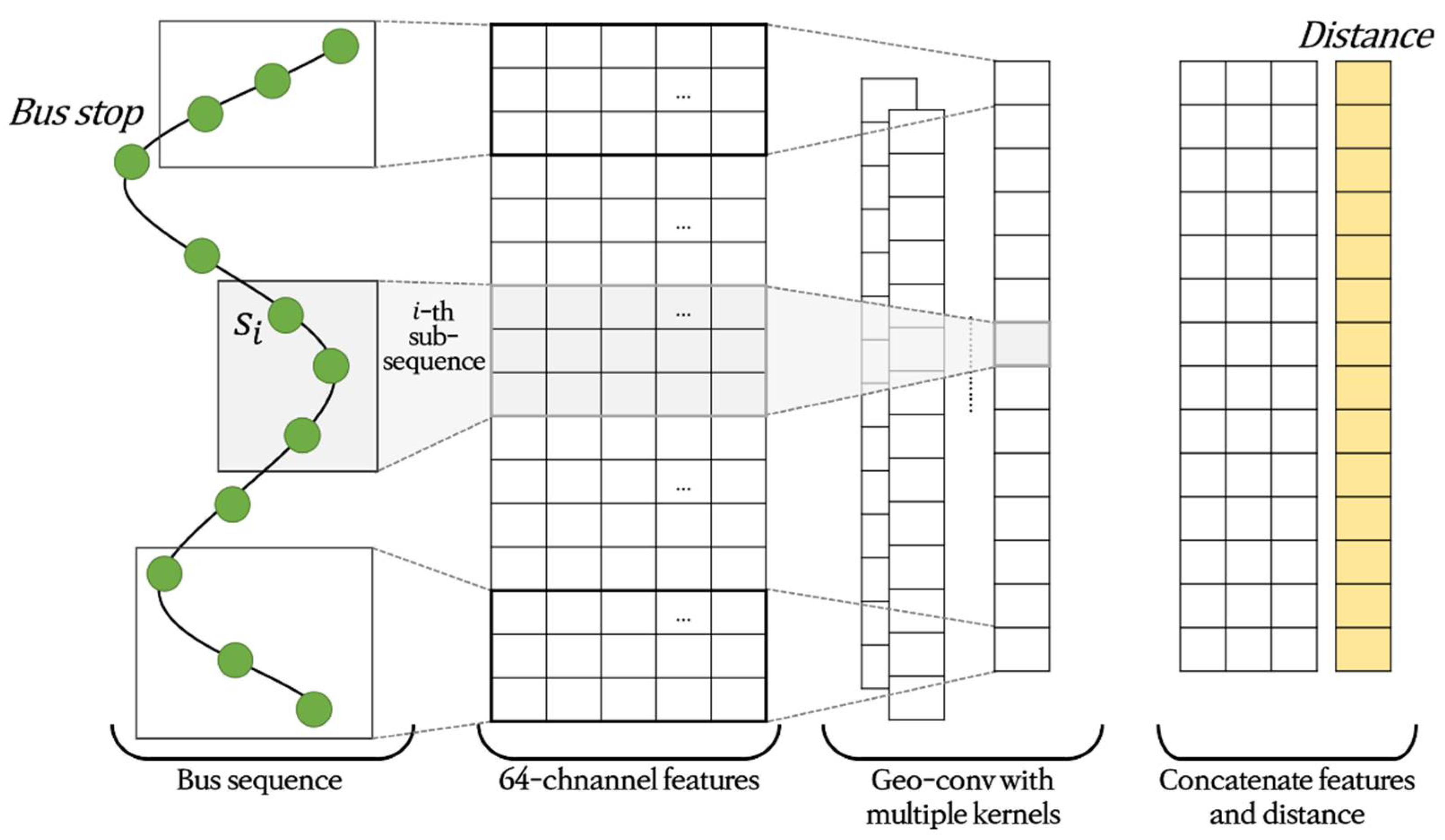
3.2.2. Spatio-Temporal Module

The spatio-temporal module consists of two layers. The first one is a geo-convolution layer that transforms the stop features (latitude, longitude, etc.) into a feature map. The second is a layer that learns the temporal characteristics of the feature map that have been extracted from the geo-convolution layer.

• Geo-convolution Layer.

The trajectory $S=\left\{s_i,\cdots ,s_j\right\}$ represents the sequence of stops that a bus has traveled, where $s_i$ is each stop $i$. $s_i$ contains information such as latitude, longitude, the number of passengers, and the link speed of the stop $i$. Capturing the spatial features from this trajectory is a very important part in the prediction of bus travel time. Convolution layers have been widely used to capture these spatial features. A typical convolution layer comprises multiple convolution filters, and each filter extracts spatial features via a convolution operation while moving at a fixed interval. In previous studies [43,55], when applying a convolution layer to a geographic object, the spatial features were extracted by dividing the space into grids and performing a convolution operation–such as image pixels–on each grid. However, in this case, incorrect spatial features may be captured depending on the size of the grid. If the size of the grid is too large, a convolution operation is performed on too much information at once, and important spatial features may be ignored. In the opposite case, the information is too sparse, making it difficult to extract the desired spatial features. Thus, we do not map the coordinates of the stops to the grid, but instead perform a convolution operation for each stop as a single cell through the geo-convolution layer. Figure 3 illustrates how the operation of the geo-convolution layer proceeds.

Before the convolution operation is implemented, the spatial features of a stop $i$ on the route can be mapped through a non-linear function, as shown in Equation (1). The present study maps the features into 64 dimensions ($st{a}_i\in R^{64}$).

$$\begin{array}{ll}st{a}_i=\tanh (W_{sta}& ·[s_{i.lat}·s_{i.lng}·s_{i.getON}·s_{i.getOFF}·s_{i.boarding}·s_{i.othergetON}·s_{i.othergetOFF}·s_{i.speed}·s_{i.lanes}\\ & ·s_{i.temp}·s_{i.preci}\left]\right),\end{array}$$

(1)

where $·$ denotes a concatenate operation, $W_{sta}$ denotes a learning weight matrix, and $st{a}_i\in R^{64}$. Thus, the output sequence corresponding to the path is in the form of $sta\in R^{64\times \left|S\right|}$, and it can be expressed as a set of non-linear mapping results for each stop. We use 1D-CNN, and the parameter matrix for the feature proceeds by sliding the stop sequence by one window. The $i$-th operation result can be expressed as Equation (2).

$$st{a}_i^{conv}=\sigma \left(W_{conv}\ast st{a}_{i:i+k-1}+b\right)$$

(2)

where ∗ is the convolution operation, b is bias, $st{a}_{i:i+k-1}$ indexes the subsequence from stop $i$ to $i+k-1$, and σ denotes the activation function. In other words, $st{a}_i^{conv}$ represents the extracted spatial features of the sequence from stop $i$ to $i+k-1$. However, since the stops correspond to one cell, the geographical distance between the two stops, which is essential for travel time prediction, is not taken into consideration. Therefore, the distance ${\displaystyle \sum }_{j=i+1}^{j+k-1}D\left(s_{j-1},s_j\right)$ of the subsequence is added to the output of the convolution operation. As a result, the shape of the output of the geo-convolution layer is $R^{\left(c+1\right)\left(\left|S\right|-k+1\right)}$, and $c$ is the number of convolution filters.

• Recurrent Layer.

In this study, a recurrent layer is introduced to capture the temporal dependency between subsequences. A recurrent neural network is a particular neural network that predicts the future using current and past data. It has a structure in which the output at time $\left(t-1\right)$ affects the output at time $t$. These features make processing data that appear sequentially (e.g., voice, text, and time-series data) suitable. The recurrent neural network tracks the previous output values and adjusts a weight. As the tracking length increases, the gradient vanishes, and the learning ability deteriorates. Hochreiter and Schmidhuber [60] proposed LSTM to overcome this long-term dependency problem. Compared to a vanilla recurrent neural network, the cell-state concept is applied in LSTM, and information from the previous state is maintained through the cell-state. The LSTM gates learn how much to take the state of the previous cell-state. The feature map of the subsequence derived from the geo-convolution layer can calculated by Equations (3)–(6).

$$I_i=\sigma \left(W_I·\left[h_{i-1}, st{a}_i^{conv}, attr\right]+b_I\right)$$

(3)

$$F_i=\sigma \left(W_F·\left[h_{i-1}, st{a}_i^{conv}, attr\right]+b_F\right)$$

(4)

$$O_i=\sigma \left(W_O·\left[h_{i-1}, st{a}_i^{conv}, attr\right]+b_O\right)$$

(5)

$${\tilde{C}}_i=\tanh \left(W_C·\left[h_{i-1}, st{a}_i^{conv}, attr\right]+b_C\right)$$

(6)

where $W_I$, $W_F$, $W_O$, and $W_C$ are the weight matrices for the input $\left[st{a}^{conv}, attr\right]$ and the hidden state ($h$) of each gate, and $b_I$, $b_F$, $b_O$, and $b_C$ indicate the bias vector of each gate. σ is the activation function of the gate, and usually uses a sigmoid function. After the operation of each gate is completed, the cell ($C$) and hidden state ($h$) are updated by Equation (7):

$$C_i=F_i\odot C_{i-1}+I_i\odot {\tilde{C}}_i$$

(7)

According to the learned rate of the forget gate, the cell-state of the previous time step ($C_{i-1}$) is stored in the cell-state of the current time step ($C_i$), and $I_i\odot {\tilde{C}}_i$ is added. According to Equation (8), the calculated cell-state ($C_i$) is mapped to the tanh function and converted to a value between −1 and 1. Then, it is multiplied by the ratio learned from the output gate to derive the final state (hidden state).

$$h_i=O_i\odot \tanh \left(C_i\right)$$

(8)

3.2.3. Prediction Module

Since the length of the sequence derived by the spatio-temporal module differs depending on the departure and arrival stops of the path, we first need to convert it into a vector of fixed length. The simplest method is to use the arithmetic mean of the sequence values (Equation (9)):

$$h_{mean}=\frac{1}{\left|P\right|-k+1}{{\displaystyle \sum }}_{i=1}^{\left|P\right|-k+1}{h}_i$$

(9)

However, the limitation of this method is that all the values of a sequence are considered to have the same weights, and in reality, actual road congestion or passengers do not follow the same pattern at all stops and appear more frequently at certain stops. We applied the attention mechanism formulated in Equation (10), which weights the values of a sequence:

$$h_{attr}={{\displaystyle \sum }}_{i=1}^{\left|P\right|-k+1}{\alpha }_i·h_i,$$

(10)

where ${\alpha }_i$ represents the weight of the $i$-th subsequence, which is updated through the learning process. The sum of A is equal to 1. For learning the parameter ${\alpha }_i$, the features of the entire path and the spatial features of the $i$-th subsequence are used. Equations (11) and (12) can be written as follows:

$$z_i=<{\sigma }_{attr}\left(attr\right), h_i>,$$

(11)

$${\alpha }_i=\frac{e^{z_i}}{{{\displaystyle \sum }}_j^{}{e}^{z_j}},$$

(12)

where attr comprises all the path features that contain external factors, and $h_i$ is the spatio-temporal features of the subsequence. < > represents the inner product, and ${\sigma }_{attr}$ denotes a non-linear mapping function to match the dimensions of attr and $h_i$.

The final $h_{attr}$ is transferred to any residual fully connected layers that are the same size. The $i$-th layer is denoted by ${\sigma }_{f_i}$. The result of the ($i$ + 1)th layer can be denoted by $x\oplus {\sigma }_{f_{i+1}}\left(x\right)$ when the input value passing through the $i$-th layer is $x$, where $\oplus$ represents element-wise add operation. By passing through the last layer, the prediction value is obtained.

4. Experiments

4.1. Experiment Setting

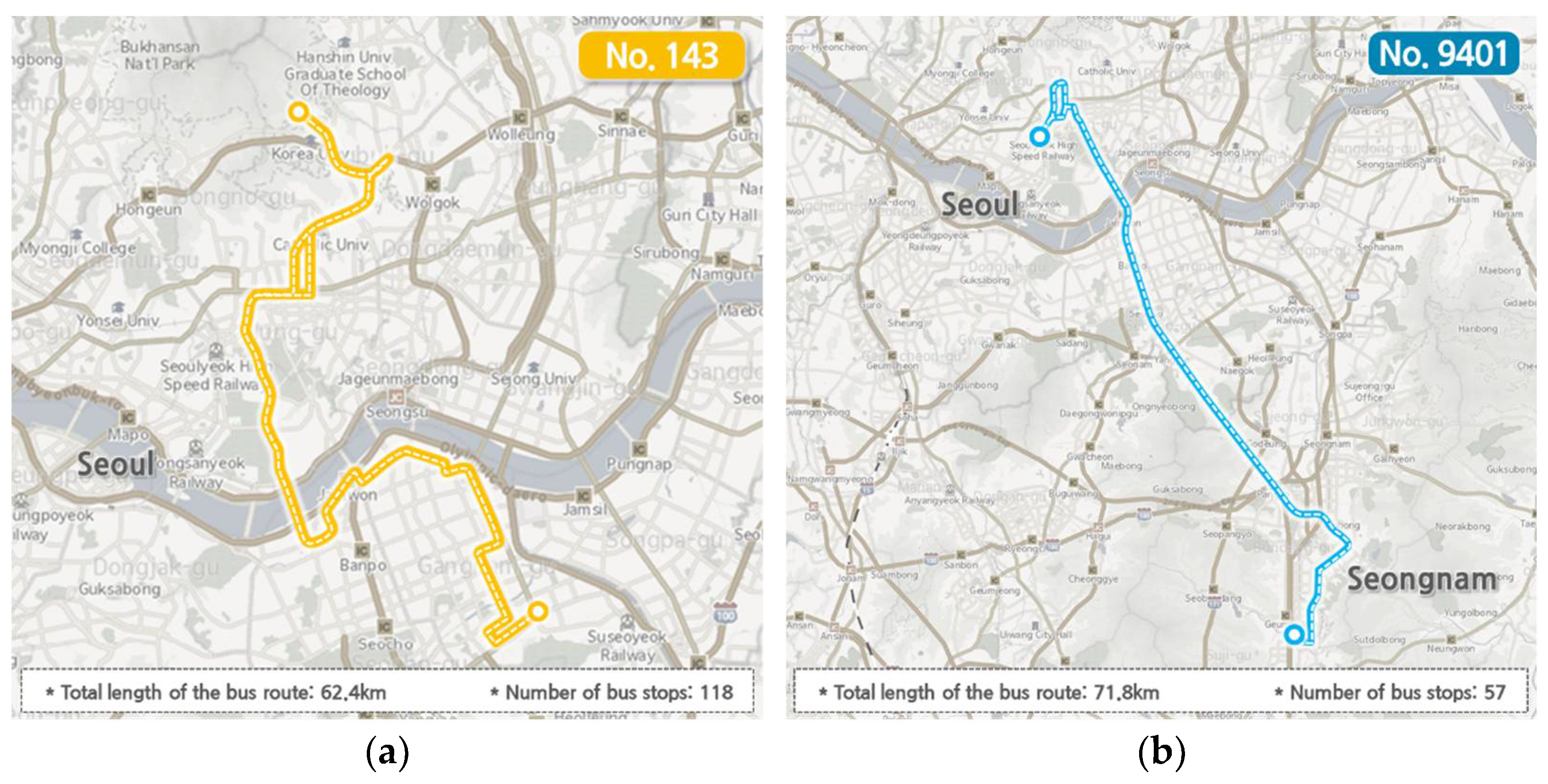
4.1.1. Dataset

In the present section, we evaluate the using smart card data from the Seoul Metropolitan Area for a three-month period from May to July 2020. Among the different bus lines, No. 143 and No. 9401 were used for evaluation. The No. 143 bus runs through the major arterial roads of the city center, whereas the No. 9401 bus is an inter-regional bus that runs between Seongnam and Seoul (it takes highways for inter-regional travel). Those two lines have 118 and 57 bus stops, respectively. A detailed route map is visualized in Figure 4.

For each operation, the number of passengers boarding or alighting the bus and the number of passengers on board at each stop were counted. We define the time at which the first ride at a stop is recorded as the time indicating when the bus arrived at that stop. In addition, we determine the speed of the road on which the stop is located via the standard node link speed data from the National Transport Information Center, which are taken at 5-min intervals. Finally, we use temperature and precipitation information obtained from the Open Meteorological Data Portal. During the research period, 1,856,015 trips and 652,307 trips were made on route, respectively. An example dataset is in the Appendix A.

Table 3. Descriptive statistics of the variables.

Route		No. 143 (Local Bus)			No. 9401 (Inter-Regional Bus)
		N	Mean	S.D.	N	Mean	S.D.
Travel distance (km/trip)		1,856,015	3.96	3.54	652,307	23.15	8.79
Travel time (min/trip)		1,856,015	15.84	14.55	652,307	35.72	20.72
On board passenger		1,856,015	14.77	9.33	652,307	18.64	13.47
Boarding passengers	Target bus	1,856,015	2.37	2.97	652,307	2.26	3.22
	Other bus	1,856,015	11.94	13.71	652,307	5.45	8.03
Alighting passengers	Target bus	1,856,015	2.34	2.63	652,307	2.32	3.53
	Other bus	1,856,015	11.48	12.59	652,307	5.84	10.07
Link speed (km/h)		1,856,015	25.40	11.38	652,307	30.76	13.09
Link lanes		1,856,015	3.06	1.24	652,307	3.37	1.12
Temperature (°C)		1,856,015	22.97	4.73	652,307	22.34	4.73
Precipitation (mm)		1,856,015	0.19	1.22	652,307	0.15	0.97

presents the descriptive statistical results of selected variables.

4.1.2. Hyperparameters

The hyperparameters in our experiment can be described as follows:

• In the attribute module, we embed carID to $R^5$, timeID to $R^8$, and weekday to $R^3$.
• In the geo-convolution layer, we fix the number of filters $c$ at 128, the channel size at 64, and the kernel size at 3. The ELU function is used as the activation function for ${\sigma }_{conv}$.
• In the recurrent layer, we fix the hidden state size at 256 and the number of LSTM layers at 2.
• Finally, in the prediction layer, we fix the number of residual fully connected layers at 3 and the size at 256.

Additionally, for both routes, we use the dataset from 1 May to 19 July 2020 as the training set and the remainder (from 20 July to 29 July) as the test set. Consequently, it turned out that there are 1,645,110 training data and 210,904 test data for No. 143; for No. 9401, there are 602,880 training data and 49,427 test data. We adopt the Adam optimizer to train the model (learning rate = 0.001 and batch size = 512) and train the model for 20 epochs.

4.1.3. Metrics

We adopt three widely used metrics to evaluate the model performance: the Root Mean Square Error (RMSE), Mean Absolute Error (MAE), and Mean Absolute Percentage Error (MAPE):

$$\mathrm{RMSE}=\sqrt{\frac{1}{n}{\displaystyle \sum }_{i=1}^n{\left(y_t-{\widehat{y}}_t\right)}^2},$$

(13)

$$\mathrm{MAE}=\frac{1}{n}{\displaystyle \sum }_{i=1}^n\left|y_t-{\widehat{y}}_t\right|,$$

(14)

$$\mathrm{MAPE}=\frac{1}{n}{\displaystyle \sum }_{i=1}^n\frac{\left|y_t-{\widehat{y}}_t\right|}{y_t}\times 100,$$

(15)

where $y_t$ is the ground truth, and ${\widehat{y}}_t$ is the predicted value.

4.1.4. Baseline Methods

Since there is little research related to deep learning-based bus travel time predictions, we compared the performance of our model to simple baseline methods and then evaluated the model by focusing on the influence of various incorporated variables. We selected two specific models as reference models, including:

• AVG: A simple average of the pairs of departure/arrival travel times shown in the training data set.
• Geo-convRNN: A simplified model of our model. We replace the LSTM layer used to incorporate the temporal dependence in the spatio-temporal layer with the vanilla RNN layer.
• Geo-convGRU: We replace the LSTM layer of the model with a Gated Recurrent Unit (GRU) layer. A GRU is a recurrent neural network proposed by Cho et al. [61] to solve the long-term dependency problems of RNN. It is similar to the LSTM layer in that it adopts the gate concept in the information transfer process. Therefore, although there are differences in the structural aspects of the GRU and LSTM layers, they perform similarly in that they use the same concept of storing information through the gate [62].

4.2. Experiment Results

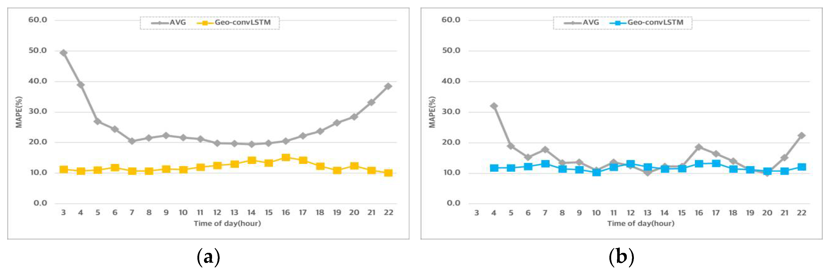
4.2.1. Performance Comparison

Table 4. Performance comparison of bus travel time predictions.

Route	No. 143 (Local Bus)			No. 9401 (Inter-Regional Bus)
Metrics	RMSE (s)	MAE (s)	MAPE (%)	RMSE (s)	MAE (s)	MAPE (%)
AVG	706.33	200.97	22.97	673.61	459.59	18.88
Geo-convRNN	575.15	151.42	16.78	490.74	341.41	17.12
Geo-convGRU	479.78	76.22	12.95	377.58	256.14	12.71
Geo-convLSTM	433.36	67.64	12.37	358.62	247.74	11.93

shows the performance comparison results between the baseline methods and our model. The Geo-convLSTM model predicted the bus travel time the most accurately; the error rates were 12.37% and 11.93% for No. 143 and No. 9401, respectively. The AVG model, which predicted the travel time by averaging past histories, was the most inaccurate. The Geo-convRNN model in which the LSTM layer was replaced with the vanilla RNN layer showed that the error rates were 4.41% and 5.19% higher than the Geo-convLSTM model for No. 143 and No. 9401, respectively. Geo-convGRU is a model in which the LSTM layer is replaced with a GRU layer with the same conditions. Compared to the Geo-convLSTM model, the error rates were 0.58% and 0.78% higher for No. 143 and No. 9401, respectively. Therefore, the following analysis is based on Geo-convLSTM. Comparing the accuracy of the two routes, No. 143, which runs in the city center, was predicted to be closer to the actual observation values than No. 9401, which runs on an inter-regional route.

We then compared the performance of the model according to the bus travel distance (Figure 5). The error rate pattern according to the bus travel distance was different for each bus line. Regarding No. 143, the error rate tended to decrease as the bus’s travel distance increased, but the error rate increased slightly when travel distance exceeded 20 km. On the other hand, No. 9401 had the highest error rate, which was observed to be in the interval of 5 to 10 km, and the error rate continued to decrease when the bus travel distance exceeded 10 km. One possible explanation for this is that the No. 143 bus mainly operates to serve inside the city center, so the travel distance is relatively short, with the rate of travel over 20 km being 0.37% (778 of 210,904 test data). Since the portion of long-distance traffic was very tiny, the training to account for long-distance travel was insufficient, and thus, the error rate was higher. Conversely, the No. 9401 bus–the inter-regional bus–had a relatively low rate of short trips between 5 to 10 km. Short trips only accounted for 3.43% of the trips taken on that bus (1695 cases out of 49,427 cases in test data), with the vast majority of cases representing long-distance trips that are over 20 km (80.41%, and 39,745 out of 49,427 cases in the test data).

In Figure 6, we compared the error rates according to the bus departure time. The error rate of the No. 143 bus increased over time, and in particular, the error rate peaked at around 4–5 p.m. The error rate of the buses departing at 6 am was the highest during the AM period. The total operating time for the No. 143 bus was 1 h 00 min, which corresponds to the one-hour peaks. During the two peak hour periods (AM and PM), many people commute to work/school and then return home, causing heavy traffic congestion compared to off-peak hours. This may hint that it is hard to make accurate predictions in such a complex situation. The No. 9401 bus showed a high error rate in the travel time for buses departing in the morning and PM peak hours, but it appears that there were no significant differences in terms of time.

4.2.2. Effect of Variables

Our model used various variables that affected the dwelling time and transit time. We evaluated the effectiveness of the variables based on three error rates by eliminating each of them independently. Not surprisingly, as shown in

Table 5. Effects of different variables.

Line	No. 143 (Local Bus)			No. 9401 (Inter-Regional Bus)
Metrics	RMSE (s)	MAE (s)	MAPE (%)	RMSE (s)	MAE (s)	MAPE (%)
Geo-convLSTM	433.36	97.64	12.37	358.62	247.74	11.93
Eliminate passenger variables	449.12	121.07	13.71	453.61	316.61	14.50
Eliminate link variables	449.97	127.70	14.87	552.56	363.68	15.42
Eliminate weather variables	435.76	102.53	12.65	396.20	367.14	12.45

, both lines had the lowest error rate when all the features were incorporated. When the passenger-related variables were excluded, the error rate for both lines increased by 1.34% and 2.57%, respectively, compared to the reference model. Meanwhile, when the link-related variables (link speed, number of lanes) were eliminated from the complete model, the error rate was relatively high, 14.87% and 15.42%, which can be viewed as a larger increase than what we observed after eliminating the passenger variables. Conversely, even though only the weather variables were eliminated while the passenger variables and link variables were maintained in the model, the error rate increased to 12.65% and 12.45%, respectively, but no significant differences were observed in our model. In this regard, it can be seen that the link features are important for effectively predicting bus travel time. Our explanation is that transit time accounts for a larger proportion of a bus’s total travel time than the dwelling time does, and delays caused by road congestion are well-reflected via the link speed.

5. Conclusions

In this study, we predicted bus travel times using a deep learning approach. We developed a Geo-conv LSTM model that the extracts spatial features of subsequences via 1D-CNN for the entire bus travel sequence and that captures the temporal dependencies between subsequences using the LSTM network. To specify the bus travel time, we divided it into the dwelling time (the number of boarding or alighting passengers) and transit time (combining factors such as running speed and the number of lanes at a stop). In addition, the external factors that are expected to affect travel time such as the travel departure time, the vehicle identification number, the day of the week, and the weather were also taken into consideration.

The constructed model was evaluated using actual behavioral data sources: smart card data from the Seoul Metropolitan Area for three months from May to July 2020. Among the bus lines, two specific bus lines–No. 143 (local bus) and No. 9401 (inter-regional bus)–were used for evaluation. We compared the performance of the AVG model and the Geo-convRNN model, a convGRU model in which the LSTM layer is replaced with a vanilla RNN and GRU, respectively, as baseline models. The results show that our model outperformed the other reference models. Specifically, the performance varied according to the type of bus line. The models showed slightly lower performance for the No. 143 bus when the travel distance exceeded 20 km; for the No. 9401 bus, lower performance was observed when we estimated short-distance intervals along the route. Buses operating at peak hours were found to have a relatively high error rate; nevertheless, no significant differences were observed regarding the day of the week. Lastly, we compared the effectiveness of the variables that were incorporated into the prediction model. When the variables related to the link of the stop location were eliminated, the error rate tended to increase the most, evidently suggesting that it plays an important role in the prediction of travel time.

Of course, our research has several limitations. First, our model does not account for features other than the stops when predicting travel time. Delays caused by boarding and alighting the bus tend to accumulate along with the progression of the stop sequence, and the link state is also strongly affected by the state of the connected links. Additionally, the spatial features were only extracted at the stop coordinates, and the path features between stops were ignored when estimating the travel time by composing a subsequence for an entire stop sequence. Thus, it would be desirable to understand the connectivity of a stop or road using a graph convolution neural network or graph embedding method. Ultimately, we believe that not only should the stop feature be predicted, but the features of the connected roads and adjacent stops should also be predicted and could be incorporated into bus travel time predictions.

References

1. United Nations; Department of Economic and Social Affairs, Population Division. World Urbanization Prospects: The 2018 Revision (ST/ESA/SER. A/420); United Nations: New York, NY, USA, 2019. [Google Scholar]
2. Kuramochi, T.; Elzen, M.; Peters, G. Global Emissions Trends and G20 Status and Outlook; United Nations: Nairobi, Kenya, 2020. [Google Scholar]
3. Ceder, A.; Wilson, N.H. Bus network design. Transp. Res. Part B Methodol. 1986, 20, 331–344. [Google Scholar] [CrossRef]
4. Lampkin, W.; Saalmans, P.D. The design of routes, service frequencies, and schedules for a municipal bus undertaking: A case study. J. Oper. Res. Soc. 1967, 18, 375–397. [Google Scholar] [CrossRef]
5. Van Oudheusden, D.L.; Ranjithan, S.; Singh, K.N. The design of bus route systems—An interactive location-allocation approach. Transportation 1987, 14, 253–270. [Google Scholar] [CrossRef]
6. Pattnaik, S.B.; Mohan, S.; Tom, V.M. Urban bus transit route network design using genetic algorithm. J. Transp. Eng. 1998, 124, 368–375. [Google Scholar] [CrossRef]
7. Vakulenko, K.; Kuhtin, K.; Afanasieva, I.; Galkin, A. Designing optimal public bus route networks in a suburban area. Transp. Res. Procedia 2019, 39, 554–564. [Google Scholar] [CrossRef]
8. Ahern, Z.; Paz, A.; Corry, P. Approximate multi-objective optimization for integrated bus route design and service frequency setting. Transp. Res. Part B Methodol. 2022, 155, 1–25. [Google Scholar] [CrossRef]
9. Nadinta, D.S.; Surjandari, I.; Laoh, E. A Clustering-based Approach for Reorganizing Bus Route on Bus Rapid Transit System. In Proceedings of the 2019 16th International Conference on Service Systems and Service Management (ICSSSM), Shenzhen, China, 13–15 July 2019; IEEE: Piscataway, NJ, USA, 2019. [Google Scholar]
10. Benn, H.P. No. Project SA-1; Bus Route Evaluation Standards. Transportation Research Board: Washington, DC, USA, 1995.
11. Liu, W.; Teng, J.; Zhang, D. Performance evaluation at bus route level: Considering carbon emissions. In Proceedings of the ICTE 2013: Safety, Speediness, Intelligence, Low-Carbon, Innovation, Chengdu, China, 19–20 October 2013; ASCE: Reston, VA, USA, 2013. [Google Scholar]
12. Simonelli, F.; Tinessa, F.; Marzano, V.; Papola, A.; Romano, A. Laboratory experiments to assess the reliability of traffic assignment map. In Proceedings of the 2019 6th International Conference on Models and Technologies for Intelligent Transportation Systems (MT-ITS), Carcow, Poland, 5–7 June 2019; IEEE: Piscataway, NJ, USA, 2019. [Google Scholar]
13. Jiménez, F.; Román, A. Urban bus fleet-to-route assignment for pollutant emissions minimization. Transp. Res. Part E Logist. Transp. Rev. 2016, 85, 120–131. [Google Scholar] [CrossRef]
14. Mori, U.; Mendiburu, A.; Álvarez, M.; Lozano, J. A review of travel time estimation and forecasting for advanced traveller information systems. Transp. A Transp. Sci. 2015, 11, 119–157. [Google Scholar] [CrossRef]
15. Schmitt, E.J.; Jula, H. On the limitations of linear models in predicting travel times. In Proceedings of the 2007 IEEE Intelligent Transportation Systems Conference, Bellevue, WA, USA, 30 September–3 October 2007. [Google Scholar]
16. Chung, E.H.; Shalaby, A. Expected Time of Arrival Model for School Bus Transit Using Real-Time Global Positioning System-Based Automatic Vehicle Location Data. J. Intell. Transp. Syst. 2007, 11, 157–167. [Google Scholar] [CrossRef]
17. Sun, D.; Luo, H.; Fu, L.; Liu, W.; Liao, X.; Zhao, M. Predicting Bus Arrival Time on the Basis of Global Positioning System Data. Transp. Res. Rec. 2007, 2034, 62–72. [Google Scholar] [CrossRef] [Green Version]
18. Petersen, N.C.; Rodrigues, F.; Pereira, F.C. Multi-output bus travel time prediction with convolutional LSTM neural network. Expert Syst. Appl. 2019, 120, 426–435. [Google Scholar] [CrossRef] [Green Version]
19. Skabardonis, A.; Geroliminis, N. Real-time Estimation of Travel Times on Signalized Arterials. Transp. Traffic Theory 2005, 387–406. Available online: https://os.zhdk.cloud.switch.ch/tind-tmp-epfl/c148e9a2-1df4-4e67-b494-f3acff299bd0?response-content-disposition=attachment%3B%20filename%2A%3DUTF-8%27%27Skab.Gerol.2005.pdf&response-content-type=application%2Fpdf&AWSAccessKeyId=ded3589a13b4450889b2f728d54861a6&Expires=1655274384&Signature=Uq00mE1PrpvqlANheA0grD7chH8%3D (accessed on 15 March 2022).
20. Bai, M.; Lin, Y.; Ma, M.; Wang, P. Travel-Time Prediction Methods: A Review. In Smart Computation and Communication; Springer: Berlin/Heidelberg, Germany, 2018; pp. 67–77. [Google Scholar]
21. Kwon, J.; Coifman, B.; Bickel, P. Day-to-Day Travel-Time Trends and Travel-Time Prediction from Loop-Detector Data. Transp. Res. Rec. 2000, 1717, 120–129. [Google Scholar] [CrossRef]
22. Zhang, X.; Rice, J.A. Short-term travel time prediction. Transp. Res. Part C Emerg. Technol. 2003, 11, 187–210. [Google Scholar] [CrossRef]
23. Nikovski, D.; Nishiuma, N.; Goto, Y.; Kumazawa, H. Univariate short-term prediction of road travel times. In Proceedings of the 2005 IEEE Intelligent Transportation Systems, Vienna, Austria, 16 September 2005. [Google Scholar]
24. Abdelfattah, A.M.; Khan, A.M. Models for predicting bus delays. Transp. Res. Rec. 1998, 1623, 8–15. [Google Scholar] [CrossRef]
25. Patnaik, J.; Chien, S.; Bladikas, A. Estimation of Bus Arrival Times Using APC Data. J. Public Transp. 2004, 7, 1–20. [Google Scholar] [CrossRef] [Green Version]
26. Jeong, R.; Rilett, L.R. Prediction Model of Bus Arrival Time for Real-Time Applications. Transp. Res. Rec. 2005, 1927, 195–204. [Google Scholar] [CrossRef]
27. Agafonov, A.A.; Yumaganov, A.S. Bus Arrival Time Prediction Using Recurrent Neural Network with LSTM Architecture. Opt. Mem. Neural Netw. 2019, 28, 222–230. [Google Scholar] [CrossRef]
28. Chien, S.I.; Ding, Y.; Wei, C. Dynamic Bus Arrival Time Prediction with Artificial Neural Networks. J. Transp. Eng. 2002, 128, 429–438. [Google Scholar] [CrossRef]
29. Chen, M.; Liu, X.; Xia, J.; Chein, S.I. A Dynamic Bus Arrival Time Prediction Model Based on APC data. Comput. Aided Civ. Infrastruct. Eng. 2004, 19, 364–376. [Google Scholar] [CrossRef]
30. Oda, T. An Algorithm for Prediction of Travel Time Using Vehicle Sensor Data. In Proceedings of the Third International Conference on Road Traffic Control, London, UK, 22–24 March 1994. [Google Scholar]
31. Guin, A. Travel Time Prediction Using a Seasonal Autoregressive Integrated Moving Average Time Series Model. In Proceedings of the 2006 IEEE Intelligent Transportation Systems Conference, Toronto, ON, Canada, 17–20 September 2006. [Google Scholar]
32. Xia, J.; Chen, M.; Huang, W. A Multistep Corridor Travel-Time Prediction Method Using Presence-Type Vehicle Detector Data. J. Intell. Transp. Syst. 2011, 15, 104–113. [Google Scholar] [CrossRef]
33. Yildirimoglu, M.; Ozbay, K. Comparative evaluation of probe-based travel time prediction techniques under varying traffic conditions. In Proceedings of the Transportation Research Board 91st Annual Meeting, Washington, DC, USA, 22–26 January 2012; Transportation Research Board: Washington, DC, USA, 2012. [Google Scholar]
34. Osman, O.; Rakha, H.; Mittal, A. Application of Long Short Term Memory Networks for Long- and Short-Term Bus Travel Time Prediction. Available online: https://www.preprints.org/manuscript/202104.0269/v1 (accessed on 15 March 2022).
35. Wu, C.H.; Ho, J.M.; Lee, D.T. Travel-Time Prediction with Support Vector Regression. IEEE Trans. Intell. Transport. Syst. 2004, 5, 276–281. [Google Scholar] [CrossRef] [Green Version]
36. Vanajakshi, L.; Rilett, L.R. Support Vector Machine Technique for the Short Term Prediction of Travel Time. In Proceedings of the 2007 IEEE Intelligent Vehicles Symposium, Istanbul, Turkey, 13–15 June 2007. [Google Scholar]
37. Bin, Y.; Zhongzhen, Y.; Baozhen, Y. Bus Arrival Time Prediction Using Support Vector Machines. J. Intell. Transp. Syst. 2006, 10, 151–158. [Google Scholar] [CrossRef]
38. Bai, C.; Peng, Z.R.; Lu, Q.C.; Sun, J. Dynamic Bus Travel Time Prediction Models on Road with Multiple Bus Routes. Comput. Intell. Neurosci. 2015, 2015, 432389. [Google Scholar] [CrossRef] [PubMed] [Green Version]
39. Wang, J.Y.; Wong, K.I.; Chen, Y.Y. Short-term Travel Time Estimation and Prediction for Long Freeway Corridor using NN and regression. In Proceedings of the 2012 15th International IEEE Conference on Intelligent Transportation Systems, Anchorage, AK, USA, 16–19 September 2012. [Google Scholar]
40. Tak, S.; Kim, S.; Oh, S.; Yeo, H. Development of a Data-Driven Framework for Real-Time Travel Time Prediction. Comput. Aided Civ. Infrastruct. Eng. 2016, 31, 777–793. [Google Scholar] [CrossRef]
41. Hou, Y.; Edara, P. Network Scale Travel Time Prediction using Deep Learning. Transp. Res. Rec. 2018, 2672, 115–123. [Google Scholar] [CrossRef]
42. Zhang, H.; Wu, H.; Sun, W.; Zheng, B. DeepTravel: A Neural Network Based Travel Time Estimation Model with Auxiliary Supervision. arXiv 2018, arXiv:1802.02147. [Google Scholar]
43. Li, L.; Jiang, X. Predicting the Travel Time in Using Recurrent Neural Networks: A Case Study of Fuzhou. In Proceedings of the Advances in Smart Vehicular Technology, Transportation, Communication and Applications, Kaohsiung, Taiwan, China, 6–8 November, 2017; Springer: Berlin/Heidelberg, Germany, 2017; Volume 86. [Google Scholar]
44. Wei, W.; Jia, X.; Liu, Y.; Yu, X. Travel Time Forecasting with Combination of Spatial-Temporal and Time Shifting Correlation in CNN-LSTM Neural Network. In Proceedings of the Web and Big Data, Macau, China, 23–25 July 2018; Springer: Berlin/Heidelberg, Germany, 2018. [Google Scholar]
45. Wang, Z.; Fu, K.; Ye, J. Learning to Estimate the Travel Time. In Proceedings of the KDD ‘18: The 24th ACM SIGKDD International Conference on Knowledge Discovery and Data Mining, London, UK, 19–23 August 2018; ACM: New York, NY, USA, 2018. [Google Scholar]
46. Wang, D.; Zhang, J.; Cao, W.; Li, J.; Zheng, Y. When Will You Arrive? Estimating Travel Time Based on Deep Neural Networks. In Proceedings of the Thirty-Second AAAI Conference on Artificial Intelligence, New Orleans, LA, USA, 2–7 February 2018. [Google Scholar]
47. Xu, J.; Zhang, Y.; Chao, L.; Xing, C. STDR: A Deep Learning Method for Travel Time Estimation. In Proceedings of the Database Systems for Advanced Application, Chiang Mai, Thailand, 22–25 April 2019; Springer: Berlin/Heidelberg, Germany, 2019. [Google Scholar]
48. Li, X.; Wang, H.; Sun, P.; Zu, H. Spatiotemporal Features—Extracted Travel Time Prediction Leveraging Deep-Learning-Enabled Graph Convolutional Neural Network Model. Sustainability 2021, 13, 1253. [Google Scholar] [CrossRef]
49. Ye, J.; Zhao, J.; Ye, K.; Xu, C. How to build a graph-based deep learning architecture in traffic domain: A survey. IEEE Trans. Intell. Transp. Syst. 2020, 23, 3904–3924. [Google Scholar] [CrossRef]
50. Jiang, W.; Luo, J. Graph neural network for traffic forecasting: A survey. arXiv 2021, arXiv:2101.11174. [Google Scholar]
51. Fang, X.; Huang, J.; Wang, F.; Zeng, L.; Liang, H.; Wang, H. ConSTGAT: Contextual spatial-temporal graph attention network for travel time estimation at baidu maps. In Proceedings of the 26th ACM SIGKDD International Conference on Knowledge Discovery & Data Mining, Virtual Event, CA, USA, 6–10 July 2020. [Google Scholar]
52. Hong, H.; Lin, Y.; Yang, X.; Li, Z.; Fu, K.; Wang, Z.; Qie, X.; Ye, J. HetETA: Heterogeneous information network embedding for estimating time of arrival. In Proceedings of the 26th ACM SIGKDD International Conference on Knowledge Discovery & Data Mining, Virtual Event, CA, USA, 6–10 July 2020. [Google Scholar]
53. Hu, J.; Guo, C.; Yang, B.; Jensen, C.S. Stochastic Weight Completion for Road Networks using Graph Convolutional Networks. In Proceedings of the 2019 IEEE 35th International Conference on Data Engineering (ICDE), Macao, China, 8–11 April 2019; IEEE: Piscataway, NJ, USA, 2019. [Google Scholar]
54. Shao, K.; Wang, K.; Chen, L.; Zhou, Z. Estimation of Urban Travel Time with Sparse Traffic Surveillance Data. In Proceedings of the 2020 4th High Performance Computing and Cluster Technologies Conference & 2020 3rd International Conference on Big Data and Artificial Intelligence, Qingdao, China, 3–6 July 2020. [Google Scholar]
55. Shen, Y.; Jin, C.; Hua, J. TTPNet: A Neural Network for Travel Time Prediction Based on Tensor Decomposition and Graph Embedding. IEEE Trans. Knowl. Data Eng. 2020. [Google Scholar] [CrossRef]
56. Jin, G.; Yan, H.; Li, F.; Huang, J.; Li, Y. Spatio-Temporal Dual Graph Neural Networks for Travel Time Estimation. arXiv 2021, arXiv:2105.13591. [Google Scholar]
57. Liu, H.; Xu, H.; Yan, Y.; Cai, Z.; Sun, T.; Li, W. Bus Arrival Time Prediction Based on LSTM and Spatial-Temporal Feature Vector. IEEE Access 2020, 8, 11917–11929. [Google Scholar] [CrossRef]
58. Tang, K.; Chen, S.; Khattak, A.J.; Pan, Y. Deep Architecture for Citywide Travel Time Estimation Incorporating Contextual Information. J. Intell. Transp. Syst. 2021, 25, 313–329. [Google Scholar] [CrossRef]
59. Chen, C.; Wang, H.; Yuan, F.; Jia, H.; Yao, B. Bus Travel Time Prediction Based on Deep Belief Network with Back-propagation. Neural Comput. Applic 2020, 32, 10435–10449. [Google Scholar] [CrossRef]
60. Hochreiter, S.; Schmidhuber, J. Long short-term memory. Neural Comput. 1997, 9, 1735–1780. [Google Scholar] [CrossRef] [PubMed]
61. Cho, K.; Van Merriënboer, B.; Bahdanau, D.; Bengio, Y. On the properties of neural machine translation: Encoder-decoder approaches. arXiv 2014, arXiv:1409.1259. [Google Scholar]
62. Chung, J.; Gulcehre, C.; Cho, K.; Bengio, Y. Empirical evaluation of gated recurrent neural networks on sequence modeling. arXiv 2014, arXiv:1412.3555. [Google Scholar]
Figure 1. Bus travel time.
Sustainability 14 07431 g001
Figure 2. Model architecture.
Sustainability 14 07431 g002
Figure 3. Geo-convolution layer.
Sustainability 14 07431 g003
Figure 4. Route maps for the selected bus routes: (a) No. 143 (local bus); (b) No. 9401 (inter-regional bus).
Sustainability 14 07431 g004
Figure 5. Error rates by travel distance (5 km). (a) No. 143 (local bus); (b) No. 9401 (inter-regional bus).
Sustainability 14 07431 g005
Figure 6. Error rates by departure time (1 h). (a) No. 143 (local bus); (b) No. 9401 (inter-regional bus).
Sustainability 14 07431 g006