Abstract
It is of great significance to study the regional differences and temporal and spatial evolution of China’s carbon emission intensity under the carbon emissions trading mechanism, and to explore the potential for regional emission reduction. This paper uses the Theil index and Moran index to analyze the regional differences and temporal and spatial evolution trend of carbon emission intensity in China from 2010 to 2019, further constructs the emission reduction effect standard of carbon emissions trading mechanisms, discusses the emission reduction effect of the trading mechanisms, and measures the regional emission reduction potential according to the environmental learning curve. The results showed that: (1) China’s overall carbon emissions continued to increase, but the carbon emission intensity showed an overall decreasing trend. There are strong regional differences in China’s carbon emission intensity. The carbon emission intensity in the western region is higher, and the overall regional difference is decreasing year by year. (2) China’s carbon emissions trading mechanism has a significant reduction effect, but the total quota slack of the Tianjin, Beijing, and Chongqing carbon emissions trading pilot markets is loose. (3) Shanghai, Shanxi, Jiangxi, Guizhou, Inner Mongolia, and Beijing are high-efficiency carbon emission reduction provinces (more than 35%), and Fujian and Xinjiang are low-efficiency carbon emission reduction provinces (less than 15%). It is necessary to further develop the demonstration effect of high emission reduction potential areas and increase the emission reduction efforts in low emission reduction potential areas.
1. Introduction
The rapid growth of the global economy has led to a rapid increase in energy demand and consumption in various countries. The energy consumption and production activities triggered by economic development have brought about a sharp increase in total carbon emissions, resulting in severe climate and environmental problems, and have also posed new challenges to China’s sustainable development. Faced with such climate change, countries around the world began to work together to deal with it. China formulates emission reduction targets according to the actual development of each province, promotes energy conservation and emission reduction, and actively builds an international low-carbon image. China has gradually taken control of total carbon emissions aimed at achieving ‘carbon neutrality’ by 2060. By summarizing the research results of scholars on carbon emissions, it can be found that carbon emissions have certain temporal and spatial differences, which are manifested in the regional differences in carbon emission intensity [1,2]. The reasons for regional differences may come from the differences in the regional economic level, technological innovation, energy consumption, and industrial structure [3]. Due to population growth and industrialization, China’s carbon emission intensity distribution is low in the east and high in the west [4]. The pressure for carbon emission reduction in the central and western regions is large, but in recent years, the gap between the central and eastern regions has gradually narrowed. The reason is that the low-carbon economy in the eastern and central regions has a faster transformation speed, a better degree of development, and a higher degree of green finance development [5]. Therefore, it is of great significance to measure the regional differences in China’s carbon emissions, analyze the spatio-temporal evolution of carbon emissions, discuss the emission reduction effect of the carbon emissions trading mechanism, and further analyze the potential for regional carbon emission reduction for China to achieve emission reduction targets.
Carbon emissions trading mechanisms play a role in promoting carbon emission reduction targets in China. Market mechanisms can reasonably and effectively allocate carbon emission resources. Enterprises make decisions after weighing the cost of purchasing carbon emission rights and upgrading low-carbon technology. The carbon trading price and technology trading price form a supply–demand relationship. At present, China has actively introduced market mechanisms into environmental regulation and related policies. Since 2011, Beijing, Shanghai, and other regions have begun to establish a carbon emissions trading market and optimize resource allocation by market trading mechanisms. Under the market mechanism, completing quota targets through carbon emissions trading can effectively reduce emission reduction costs. Therefore, the carbon emissions trading mechanism is an important institutional innovation and policy tool for achieving carbon emission reductions [6]. On the one hand, some scholars start from the carbon emissions trading mechanism to explore whether the carbon emissions trading mechanism itself produces carbon emission reductions. The sufficient condition for its emission reduction effect is that the enterprises can obtain additional emission reduction effects by participating in carbon emissions trading [7]. For such studies, the carbon emissions trading mechanism is generally regarded as an exogenous variable, and a logical relationship is established between the total carbon emission reduction and the decline rate of the carbon emission intensity of industries or enterprises that are included in the market. For example, Xuan et al. [8] set the tightness of the total quota as an indicator of the emission reduction effect of the carbon emissions trading mechanism. Xia et al. [9] used the difference-in-differences model to analyze whether the included enterprises had emission reduction performance. Aihua et al. [10] measured the decline of carbon emission intensity by setting enterprises not included in the carbon emissions trading market as the control group, and compared the emission reduction of the two groups with the overall decline in the carbon emission intensity as a reference. In the absence of other exogenous variables, without considering other variables that may produce carbon emission reductions, the enterprise emission reduction rate and the non-enterprise emission reduction rate are analyzed. This measure eliminates the external influence to the greatest extent, and measures and analyzes the emission reduction performance of the carbon emissions trading mechanism itself. Based on the existing research, it can be found that domestic and foreign scholars analyze the level of carbon emissions in China and summarize the regional characteristics. At the same time, the emission reduction effectiveness of the carbon emissions trading mechanism is analyzed. However, there are few studies on the spatial-temporal evolution of the regional carbon emission intensity and regional emission reduction potential in China under the carbon emissions trading mechanism, which needs further exploration. This paper introduces the measurement of carbon emission intensity, the measurement of regional differences, and the identification method of influencing factors, and analyzes the spatiotemporal evolution law of carbon emission intensity. On this basis, we further discuss the impact of carbon emissions trading mechanisms on carbon emission reduction, and find that the key elements of the mechanisms play a role in carbon emission reductions. Accordingly, in the process of building a national carbon emissions trading market, it is important to set reasonable emissions quotas, and through the carbon emissions trading mechanism, realize regional carbon reduction potential to achieve China’s overall emission reduction targets. The research results can provide a reference for China to formulate low-carbon economic development and carbon emission reduction policies considering emission reduction targets and regional emission reduction potential, and provide a reference for the carbon emissions trading mechanism to actively play a role in emission reduction.
2. Research Methods
2.1. Total Carbon Emissions and Carbon Intensity Accounting
The measurement of total carbon emissions is mainly based on measurement and calculation, which can be divided into the emission factor method, quality balance method, and measurement [11]. The prevailing approach in existing studies is to use IPCC (The Intergovernmental Panel on Climate Change) accounting methods or to use existing carbon emissions estimates in existing literature studies or databases such as CEADS. However, due to the lack of data in the database, the quality balance method is widely used to measure the total amount of carbon emissions, but this method needs to use a large number of material input data in the production process of enterprises as the basis for calculation. The actual measurement method requires a large number of monitoring devices to calculate carbon emissions, and needs to be equipped with high precision measurement devices, but the process requires higher cost. Compared with other measurement methods, the emission factor method is more suitable for the measurement of regional total carbon emissions. This paper selects the emission factor method to measure the total carbon emissions.
The principle of the emission factor method is to convert different energy sources into standard coal by converting the standard coal coefficient and obtaining the total carbon emissions of such energy sources according to the product of the carbon emission coefficient and total energy consumption. Ignoring the loss in the process of processing and conversion, the total consumption of different energy sources can be converted into total carbon emissions. The energy consumption data are from China Energy Statistics Yearbook (2012–2020).
https://www.yearbookchina.com/navibooklist-n3020013309-1.html (accessed on 31 December 2021).
According to the energy consumption data, the standard coal coefficient, and the carbon emission coefficient, the Formula (1) can be used to estimate the total carbon emissions of 30 provinces in China:
In the formula, is the first energy consumption of s type of the province j in year t; is the carbon emission coefficient of the energy of s type.
The data of carbon emission coefficients and related indicators of each energy are shown in Table 1.

Table 1.
Carbon emission coefficients and related indicators.
Estimate carbon emissions from 30 provinces in China using Formula (1). After calculating the total carbon emission, the carbon emission intensity of each province is calculated according to the total regional GDP. The calculation formula is as follows:
is the total carbon emissions of the province , is the total GDP of s province .
2.2. Measurement of Regional Differences in Carbon Emissions in China
According to the division of China’s eastern, central, and western regions by the National Development and Reform Commission, the difference in carbon emissions levels between regions in China is analyzed by using the Theil entropy index. The calculation formula is as follows:
Since the relevant data of the Tibet Autonomous Region are incomplete, 30 provinces (excluding Hong Kong, Macao, Taiwan, and the Tibet Autonomous Region) in China from 2010 to 2020 are selected as the research objects. The Fourth Session of the Sixth National People’s Congress announced that China is divided into three regions: the east, the middle, and the west. The east includes 11 provinces (cities) such as Beijing, Tianjin, Hebei, Liaoning, Shanghai, Jiangsu, Zhejiang, Fujian, Shandong, Guangdong, and Hainan. The central region includes 10 provinces (cities), including Shanxi, Inner Mongolia, Jilin, Heilongjiang, Anhui, Jiangxi, Henan, Hubei, Hunan, and Guangxi; the western region includes Sichuan, Guizhou, Yunnan, Tibet, Shaanxi, Gansu, Qinghai, Ningxia, Xinjiang, and nine other provinces (cities). The formula indicates the eastern, central, and western regions divided by the policy.
In the above formula i, denotes the region, i = 1, 2, 3; GDPi denotes the GDP of region i; CEi is the total carbon emissions of the region i; CE is the total national carbon emissions; CEij and GDPit are the total carbon emissions and gross national product of the province j within the region i, respectively. Ci is the total amount of carbon emissions in the region i, T represents the overall carbon emission intensity gap in China, Twr represents the carbon emission intensity gap in a certain region, and Tbr represents the carbon emission intensity gap between different regions.
2.3. Identification of Factors Affecting Carbon Emissions
Spatial econometric models are usually used to study the spatial interaction between regional economies and geography. By reviewing and summarizing the research literature on the influencing factors of carbon emissions, it is found that many scholars have quantitatively analyzed the influence of regional location and spatial correlation factors on economic development, and established a regional model for identification [12,13,14,15]. In the construction process of the national carbon emissions trading market, Ye et al. [16] pointed out that in China’s carbon emissions trading mechanism, for the allocation of quotas, the spatial correlation analysis model can be established to comprehensively consider the basis and linkage of carbon emission reductions among different regions in China, and to pay attention to the important influence of spatial differences on carbon emission reductions.
The spatial econometric model is used to analyze the spatial cluster effect of carbon emissions and explore the influencing factors of regional differences in carbon emissions. By summarizing the research of scholars in China and abroad on the factors affecting carbon emissions, the following explanatory variables are preliminarily set:
2.3.1. Economic Development Level
GDP reflects the level of regional economic development. Taking 2000 as the base period, per capita GDP from 2011 to 2019 is calculated as a variable to measure the level of economic development, which is expressed as GDP. Regions with higher economic levels may undertake greater emission reduction tasks [17,18,19].
2.3.2. Energy Consumption
Coal is the main source of carbon emissions, and the proportion of coal consumption has an important impact on the total carbon emissions. At the same time, China’s industrialization process has caused a high dependence on fossil energy, making the total carbon emissions higher [20,21]. Therefore, the total consumption of fossil energy is set to represent the variable of energy consumption, which is expressed as EC.
2.3.3. Environmental Regulation
In the face of carbon emission reduction targets, the Chinese government vigorously promotes the emission reduction process, and rapidly develops and standardizes the carbon emissions trading mechanism. Porter’s hypothesis first pointed out the role of strict environmental regulation intensity in promoting carbon emission reductions. Referring to Rigby and Young [22,23], the natural logarithm of the cumulative number of environmental standards and environmental regulations issued in various provinces was used as a variable representing environmental regulation, which was expressed as ER.
2.3.4. Industrial Structure
The adjustment of industrial structures has great potential for carbon emission reduction. Scholars have confirmed through research that the industrial structure in a specific region is determined by the advantages of the region and the overall requirements and evolution of the national economic spatial layout. Through the industrial transfer and division of labor between regions, the relative disadvantage of the industry in the region is transformed into an advantage, and the evolution of the regional industrial structure is realized [24]. China’s industrial structure presents a high proportion of energy-intensive industries. Under the guidance of macroeconomic policies, the pursuit of energy conservation, and environmental protection industry highlights, the government promotes industrial restructuring, the pursuit of new industrialization, and high-tech industries and development [25,26]. However, attention should be paid to the control of investment and project expansion in high-tech industries in the process of industrial transformation to prevent increased energy consumption. The proportion of high-tech industry income in regional GDP is taken as the industrial structure variable, which is expressed as IS.
2.3.5. Low-Carbon Technology Innovation
The improvement of low-carbon technology innovation plays a very important role in carbon emission reduction. Based on the existing research, this paper measures the low-carbon technology innovation of enterprises, comprehensively considers the R&D ability, manufacturing ability, and output ability of enterprises, selects the number of low-carbon patents of enterprises to represent the R&D ability of enterprises, conducts crawlers in the patent database, and measures the low-carbon technology innovation with the number of low-carbon technology patents under the CPC-Y02 patent classification system [27]. The retrieval time is 15 October 2020, and the retrieval formula is (CPC = (Y02) AND (PNC = (‘CN’)). According to the year and the ownership of the enterprise, the manual classification is expressed as INOV.
2.3.6. Carbon Emissions Trading Mechanism
The direct path from carbon emissions trading mechanisms to carbon emission reductions is reflected in setting the total carbon emissions quota target and forming emission reduction constraints on key emissions units through the continuous development of carbon emissions trading mechanisms and the construction and operation of the national carbon emissions trading market. This is conducive for the pilot cities to achieve carbon emission reduction targets and drive carbon emission reduction in the surrounding areas. China has gradually established and developed a pilot market for carbon emissions trading since 2011, and started to build a national carbon emissions trading market at the end of 2017. The carbon emissions trading mechanisms are committed to the completion of China’s emission reduction targets, the reduction in the cost of carbon emission reduction in the production process of enterprises, and the attraction of more enterprises to participate in carbon trading. The carbon emissions trading mechanisms are an important system and policy tool for controlling the total amount of carbon emissions and encouraging enterprises to implement low-carbon technologies. The total trading volume of China’s 30 provinces and cities participating in the pilot market of carbon emissions trading is taken as the carbon emissions trading mechanism variable, expressed as ETS.
2.4. Spatial-Temporal Correlation Analysis of Regional Carbon Emissions in China
2.4.1. Global Spatial Autocorrelation Analysis
Global spatial autocorrelation analysis can be used to study the spatial characteristics of an attribute value in the whole region. Therefore, the Moran index is used to reveal the similarity of unit attribute values in adjacent spaces. So, we use the Moran index to test the global clustering and analyze the similarity, difference, and independence of carbon emissions in neighboring regions. The global Moran’s index is defined as follows:
where n is the total number of areas in the study area; xi and xj are observations of region i and region j, respectively; wij is the element in the spatial weight matrix, which measures the distance between the region i and region j. 30 provinces (excluding Hong Kong, Macao, Taiwan, and the Tibet Autonomous Region) in China from 2010 to 2020 are selected.
The space weight matrix is Wij, j = 1, 2, ..., n. i = 1, 2, ..., 30. Wij = 1/dij.
In the formula, yit represents the value of the variable in year t of the spatial unit i, that is, represents the annual average of the variable of unit i.
2.4.2. Geographically Weighted Regression Model
The geographically weighted regression (GWR) model introduces the geographical location of the data into the regression parameters, and uses the sub-sample data of adjacent observations to regress locally. The estimated parameters change with the change in the spatial location, and objectively reveal the difference in the driving factors of the research object with the change in the spatial location. The model is as follows:
In Formula (6): yi is the n × 1 dimension explanatory variable, xij is the n × j dimension explanatory variable matrix, βj(μi,θi) is the regression coefficient of the factor j at the regression point i, (μi,θi) is the latitude and longitude coordinates of the sample point i, εi is a random error term obeying the variance constant. The GWR model uses weighted least squares (WLS) to estimate the parameters of each observation point, and the i-point regression parameter β’(μi,θi) is:
To overcome the discontinuity of the spatial weight function, a Gaussian function is used to determine the weight function. See Formula (7):
In Formula (8), cij is the direct distance between sample i and j, b is the bandwidth, and wij is the parameter of the size of the spatial region where the sample data are located. The larger b is, the larger the spatial range of the sample is.
In this paper, we refer to the minimum information (AIC) criterion proposed by Fotheringham et al. [28] to calculate the bandwidth, as shown in Formula (9):
In Formula (9): σ is the standard error of the error estimation, tr(s) is the function of bandwidth, and is also the trace of matrix s. The minimum AIC bandwidth is the optimal bandwidth.
3. Results and Analysis
3.1. Measurement Results of Carbon Emissions
3.1.1. Provincial Carbon Emissions and Intensity
According to Formulas (1) and (2), the total carbon emissions and carbon emission intensity of 30 provinces in China in 2020 are calculated. The distribution of total carbon emissions and carbon emission intensity in 30 provinces in China in 2020 are shown in Figure 1 and Figure 2.
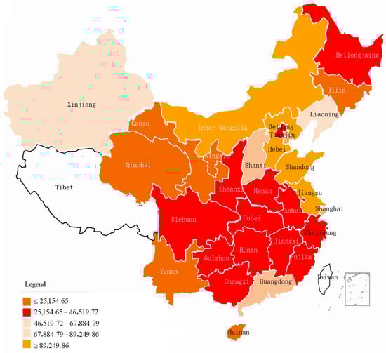
Figure 1.
Distribution of total carbon emissions in 30 provinces in China in 2020 (10,000 tons).
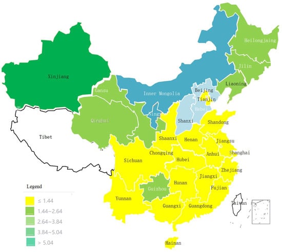
Figure 2.
Distribution of carbon emission intensity in 30 provinces in China in 2020.
The results show that there are still obvious regional differences in carbon emission intensity among different provinces in China. Inner Mongolia’s total carbon emissions and carbon emission intensity are high, with its total carbon emissions being as high as 935.544 million tons, while Ningxia’s total carbon emissions is in the middle level, but its carbon emission intensity is as high as 6.244, leading the country. The reason is that the total GDP of Ningxia province is relatively backward, and the utilization efficiency of energy is not high. The carbon emission intensity of the Beijing, Shanghai, and Guangdong carbon emissions trading pilot areas is low, and the Chongqing carbon emissions trading pilot market, as the only carbon emissions trading pilot market in the western region, has an especially low carbon emission intensity, taking a leading position in the country. Therefore, the emission reduction effect of carbon emissions trading mechanisms is obvious, and it should further play a leading role in other provinces and cities in the western region. According to China’s regional division, the total carbon emissions and carbon emission intensity differences in the eastern, central, and western regions were analyzed. According to the data of the “China Energy Statistical Yearbook” and “China Statistical Yearbook”, the corresponding regional carbon emissions and carbon emission intensity data calculated by the energy consumption and carbon emissions coefficients of each region are shown in Table 2.
Table 2.
Total Regional Carbon Emissions and Carbon Emission Intensity in China in 2020.
The difference between the carbon emission intensity of the western region and other regions shows a gradual narrowing trend, and the carbon emission intensity of the western region has had a large decline since 2016, indicating that the carbon emissions efficiency of the western region of China has improved in recent years and the effect is remarkable. However, the relatively higher carbon emission intensity in the western region is still an important reason for the slow decline of China’s overall carbon emission intensity.
3.1.2. Regional Difference Analysis of Carbon Emissions in China
This paper selects the total carbon emissions and GDP data of 30 provinces in China from 2010 to 2020 and calculates the Tell entropy index of regional carbon emission intensity according to Formulas (2) and (3), as shown in Table 3.
Table 3.
Theil entropy index of regional carbon emission intensity.
From Table 3′s data, it can be found that 2014 is a turning year for carbon emission intensity in China. In 2014, the Theil index of China’s carbon emission intensity reached its highest value, that is, the largest inter-regional difference in China’s overall carbon emission intensity. After 2014, China’s overall carbon emission intensity gap TP and regional carbon emission intensity gap Twr showed a downward trend, and the regional carbon emission intensity gap Tbr showed an increasing trend year by year. Since 2011, eight pilot carbon emissions trading markets in China have established and formulated emissions quotas and encouraged regions to increase emission reduction efforts. The trade between quotas reduces the difference in carbon emission intensity within the region. At present, cross-regional transactions cannot be carried out among the pilot markets of carbon emissions trading in China. However, with the establishment of the national carbon emissions trading market and the continuous maturity of the CCER project, the difference between groups may have a decreasing trend. Further reducing the inter-regional carbon emissions gap becomes the main task of reducing the carbon emission intensity gap. In the future, further integrating more industries through the national carbon emissions trading market and actively promoting the cooperation of CCER projects to narrow the interregional gap will be the direction of future carbon emissions trading mechanisms.
3.1.3. Emission Reduction Analysis of Carbon Emissions Trading Markets
China has gradually established and developed a pilot market for carbon emissions trading since 2011 and started to build a national carbon emissions trading market at the end of 2017. The carbon emissions trading mechanism is committed to the completion of China’s emission reduction targets, driving China’s low-carbon technology innovation and industrial structure upgrading, reducing the cost of carbon emission reductions, and attracting more enterprises to participate in carbon emission reduction. The carbon emissions trading mechanism is an important system and policy tool to control the total amount of carbon emissions and encourage enterprises to implement low-carbon technology. The impact on low-carbon technology comes from a cost-saving incentive mechanism. Enterprises incorporated in the Carbon Emissions Trading System (ETS) have legal carbon emission rights to a certain extent, based on government-issued carbon emission rights with quotas or emissions permits. After analyzing the regional measurement and spatial-temporal evolution of China’s carbon emissions, this paper focuses on the carbon emissions trading mechanism.
The control period and the experimental period are calculated based on the above formula. Since the industry is the main resource of carbon emissions and the data are relatively complete, we choose industrial energy consumption and industrial added value (Table 4) to analyze. The unit of energy consumption is ‘ten thousand tons of standard coal’, while the unit of energy consumption is ‘billion yuan’.
Table 4.
Industrial energy consumption and industrial added value of seven pilot carbon emissions trading markets in China.
According to the key elements of the carbon emissions trading mechanism, this paper explores whether the carbon emissions trading mechanism forms carbon emissions constraint behavior for the included enterprises, to analyze the regional emission reduction in China under the background of the carbon emissions trading mechanism and then explore the potential for regional emission reductions.
3.2. Identification Results of Carbon Emissions’ Influencing Factors
Given the availability of data, the data for 2011–2019 are derived from the ‘China Statistical Yearbook’, ‘China Energy Statistical Yearbook’, etc. In the space fixed effect model and time fixed effect model, ρ values are greater than 10%, so accepting the original hypothesis, the model can be simplified. The combined LM Test is in Table 5.
Table 5.
Four Effect Setting Results of SAR Panel Model.
The results of Table 4 show that in the time fixed effect model, the influence factors are more obvious. Therefore, the time fixed effect model is selected for analysis. The results show that the coefficients of lnGDP and lnEI are positive. Economic growth and energy consumption are the main factors affecting carbon emissions. Further improvements can be made in renewable energy technologies, infrastructure construction, and related energy saving policies. Higher demand for energy consumption, in the short term, should further reduce energy intensity.
The coefficients of lnER, lnINOV, lnIS, and lnETS are negative, so we can see that low-carbon technological progress is a direct means to achieve carbon emission reduction targets. With the continuous deepening of carbon emission reduction processes and the relative balance of industrial structures, improving energy efficiency with scientific and technological progress has become one of the main means and objectives of carbon emission reduction in China, and scientific and technological progress depends largely on the government‘s large investment in resources, thus helping enterprises reduce the cost of developing emission reduction technologies. The development of high-tech industry is conducive to the realization of carbon emission reduction targets in China. However, at present our country’s industrial structure still displays a large proportion of high energy consumption industries. Under the guidance of national macroeconomic policies, the development requirements of energy-saving industries are increasing. In order to promote the optimization and upgrading of industrial structures and to actively pursue new industrialization and high-tech, local governments will have a positive impact on carbon emission reduction in the long run. However, it should be noted that in the process of industrial transformation, the investment and project expansion of high-tech industries should be controlled to prevent the energy consumption caused by blind development. The industrial structure has obvious spatial spillover effects. Due to the dynamic development of industrial structures, the industrial structure between regions has also produced corresponding guidance. Carbon emission reduction is an important goal of carbon emissions trading mechanisms. Carbon emissions trading mechanisms are committed to solving the problem of excess carbon emissions, which has an important impact on carbon emission reduction and regional low-carbon economic transformations.
3.3. Analysis of the Spatial-Temporal Correlation Results of China’s Regional Carbon Emissions
3.3.1. Global Spatial Autocorrelation Analysis
The spatial correlation degree of carbon emission intensity in 30 provinces of China from 2011 to 2019 was analyzed. Table 6 is the global Moran’s index of carbon emission intensity in 30 provinces of China from 2011 to 2019.
Table 6.
Moran Index 2011–2019.
From Table 6, we can see that China’s carbon emissions have a more significant positive autocorrelation in space. Considering the characteristics of the time period, China has established a pilot market for carbon emissions trading since 2011. 2015 is the time point when the carbon emission intensity turns. Therefore, the cross-sectional data for 2011, 2015, and 2019 are selected. Based on the relevant statistical data, the LISA (Local Indicators of Spatial Association) diagram of the carbon emission intensity level of each province in China is obtained by using ArcGIS software. It reflects the local indicators of spatial connection, it explains whether there is agglomeration in the study area, including high and high agglomeration (H–H), high and low agglomeration (H–L), low and high agglomeration (L–H), and low and low agglomeration (L–L), as shown in Figure 3, Figure 4 and Figure 5.
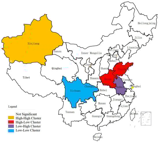
Figure 3.
Analysis of the regional carbon emissions level and Moran index in 2011.
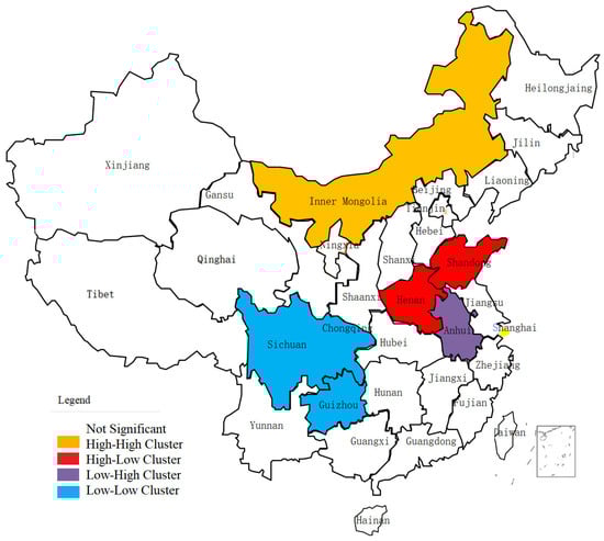
Figure 4.
Analysis of the regional carbon emissions level and Moran index in 2015.
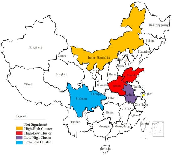
Figure 5.
Analysis of the regional carbon emissions level and Moran index in 2019.
In 2011, Xinjiang province’s (orange area) carbon emissions level were higher, but at the same time, the carbon emissions level of Xinjiang’s surrounding areas was higher. In 2015, with the continuous development and change in the economy, the distribution of carbon emission intensity in China has changed. The ‘high area’ has gradually changed from Xinjiang to Inner Mongolia (Orange area) and Ningxia (Uner Inner Mongolia), which belong to the western region of China. In 2019, the carbon intensity of China’s ‘low region’ further expanded, and the carbon reduction effect is obvious. At the same time, the ‘high and low regions’ and ‘low and high regions’ of carbon emission intensity experienced little change. In the context of the rapid and healthy development of China’s economy, we should further promote the effect of carbon emission reduction, accelerate the transfer from science and technology to productivity, and realize the regional and national carbon emissions peak as soon as possible.
3.3.2. Geographically Weighted Regression Analysis
It can be seen from Section 3.3.1 that the global Moran index of carbon emissions in 2011, 2015, and 2019 shows a trend. Therefore, the cross-sectional data of 2011, 2015, and 2019 are selected for analysis. The results are shown in Table 7. The adjusted R2 reaches more than 90%, and the fitting effect is good.
Table 7.
Overall estimation results of the GWR model.
The regression coefficients of the explanatory variables in 2011, 2015, and 2019 were calculated to analyze their spatial evolution trends.
(1) Changes in the regression coefficients of economic development levels
The regression coefficients of the economic development level in 2011, 2015 and 2019 are shown in Figure 6, Figure 7 and Figure 8.
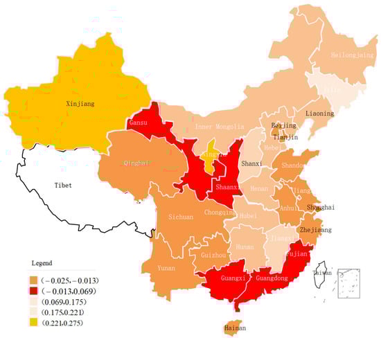
Figure 6.
Regression coefficients of economic development in 2011.
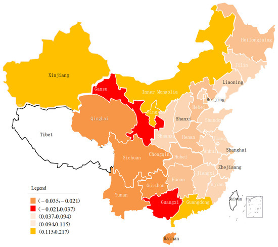
Figure 7.
Regression coefficients of economic development in 2015.
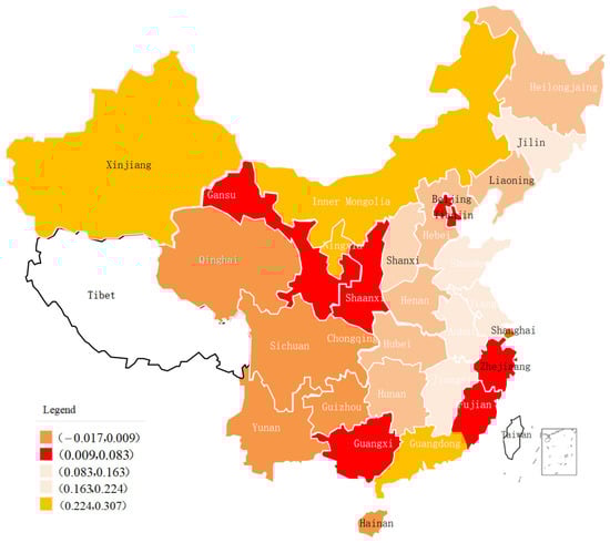
Figure 8.
Regression coefficients of economic development in 2019.
From the impact of the level of economic development on carbon emissions, the carbon emissions regression coefficient for per capita GDP in most provinces and cities is positive, and only a small number of provinces and cities have a negative impact on carbon emissions. That is, the relationship between economic development and carbon emissions in most regions has not yet entered the inflection point of the environmental Kuznets curve. With the improvement of economic development, the task of carbon emission reduction is still severe. The provinces with positive regression coefficients are mainly concentrated in Inner Mongolia, Henan, Hebei, and Heilongjiang. The carbon emissions of these provinces increase with the increase in per capita GDP, mainly because these areas still take energy consumption as the main mode of economic growth, resulting in carbon emissions increases with economic growth. In 2019, the provinces with the largest negative effect of per capita GDP on carbon emissions were mainly concentrated in Qinghai, Sichuan, and Yunnan.
(2) Energy consumption structure regression coefficient changes
The regression coefficients of the economic development level 2011, 2015 and 2019 are shown in Figure 9, Figure 10 and Figure 11.
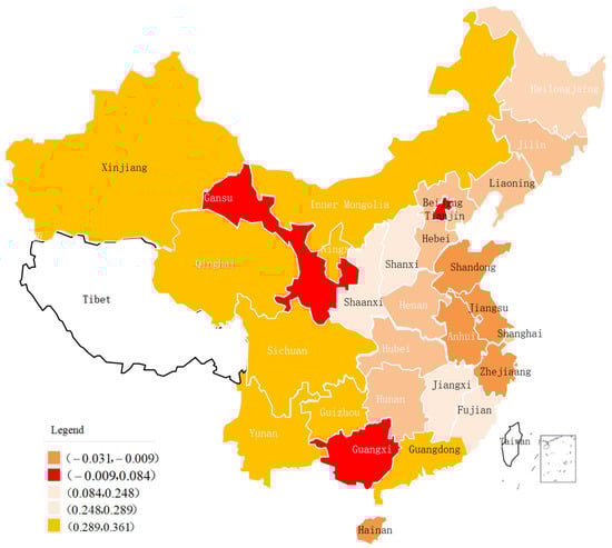
Figure 9.
Regression coefficients of the energy consumption structure in 2011.
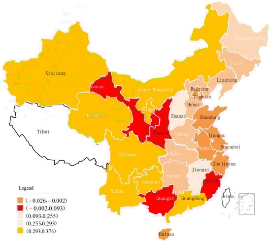
Figure 10.
Regression coefficients of the energy consumption structure in 2015.
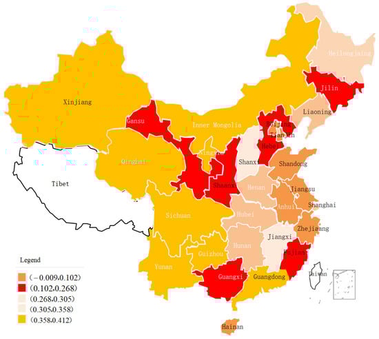
Figure 11.
Regression coefficients of the energy consumption structure in 2019.
Similarly, the regression coefficients of environmental regulation industrial structure, low-carbon technology innovation, and the carbon emissions trading mechanism in 2011, 2015, and 2019 can be obtained.
From the perspective of the impact of energy consumption on carbon emissions, the provinces with a negative impact of energy consumption on carbon emissions in 2015 were reduced to seven, and the positive regression coefficient gradually increased. In 2019, the number of provinces with a positive impact of energy consumption on carbon emissions increased to 26, with Liaoning, Jilin, and Heilongjiang having the greatest impact, respectively, and the regression coefficients were in the interval (0.305, 0.358). Thus, the difference in the regression coefficient of the impact of energy consumption on carbon emissions in neighboring provinces is small, and the energy structure adjustment in northeast China has an important impact on China’ s carbon emissions.
(3) Environmental regulation regression coefficient changes
From the perspective of the impact of environmental regulation on carbon emissions, its regression coefficient is negative, which has an important impact on carbon emissions. The regression coefficients of Shanghai, Beijing, and Zhejiang in 2011 were in the interval (−0.798, −0.833). In 2015, the regression coefficients of Shanghai and Beijing further declined, that is, the impact of environmental regulation increased. In 2019, environmental regulation had the smallest impact on Xinjiang, Liaoning, Jilin, and Hebei. Overall, the negative impact of environmental regulation on carbon emissions has gradually increased, and the gradient distribution has become more and more obvious since 2015, increasing from northeast to southwest.
(4) Changes in regression coefficients of industrial structure
From the perspective of the impact of the industrial structure on carbon emissions, the increase in the proportion of high-tech industries will not only reduce energy consumption, but also promote the upgrading of the industrial structure, which directly reduces carbon emissions. The province with the least impact of the industrial structure on carbon emissions in 2011, 2015, and 2019 are Inner Mongolia. Carbon emissions are reduced by 0.102%, 0.104%, and 0.127% for every 1% increase in the proportion of high-tech industries. The most influential provinces are Zhejiang, Guangdong, and Hebei, with regression coefficients in the interval (−0.557, −0.364).
(5) Low-carbon technology innovation regression coefficient changes
From the perspective of the impact of low-carbon technology innovation on carbon emissions, the negative effect of low-carbon technology innovation on carbon emissions began to increase in 2015, Hebei and Jiangsu were added in to the provinces with greater impact compared with 2011, and the regression coefficients increased to the interval (−0.379, −0.201). In 2015, the provinces with a large increase in the negative effect of low-carbon technology innovation on carbon emissions include Guangdong and Fujian, and the regression coefficients are in the interval (−0.286, −0.225). Overall, the impact of low-carbon technology innovation on carbon emissions has obvious spatial dependence.
(6) Carbon emissions trading mechanism regression coefficient changes
From the perspective of the impact of carbon emissions trading mechanisms on carbon emissions, the regression coefficients of most provinces are negative and have a negative impact on carbon emissions. With the deepening of the construction of carbon emissions trading markets, the total amount of market transactions has increased. More and more enterprises have participated in the market. The national carbon emissions trading market has begun to operate and be incorporated into a large number of high-emission enterprises, thereby reducing the total amount of carbon emissions. In 2011, there were five provinces with a negative impact of their carbon emissions trading mechanism. The most influential provinces are Hubei and Guangdong. For every 1% increase in trading volume, carbon emissions fell 0.093~0.118%. In 2015, the number of provinces whose carbon emissions trading mechanism had a negative impact on carbon emissions increased rapidly, and the impact gradually increased. In 2019, the number of provinces whose carbon emissions trading mechanism had a negative impact on carbon emissions increased to 12, with Hubei, Shanghai, and Guangdong having the greatest impact, respectively. The regression coefficients are in the interval (−0.156, −0.121).
4. Discussion
4.1. Evaluation of Carbon Emission Reduction Effectiveness of Carbon Emissions Trading Mechanisms
4.1.1. Measurement of Relative Emission Reduction Rates
According to the research conclusion of Wang et al. (2020) [27], the sufficient condition for judging the effectiveness of the carbon emissions trading mechanism is that the carbon emissions trading mechanism has a relative emission reduction rate, that is, the inclusion of enterprises generates an additional carbon emission reduction rate. Firstly, by setting the relative emission reduction level between the experimental group and the control group, we analyze whether additional reductions can be generated under the carbon emissions trading mechanism. We analyze the ratio of the carbon emission intensity decline level and overall carbon emission intensity decline level in the same period. Some scholars choose the industry average or regional carbon emission intensity decline level as a reference according to the research objectives, to calculate the actual carbon emission intensity decline level of enterprises. Without exogenous shocks, the effect of technological progress and other policies on emission reductions is temporarily ignored, and the overall reduction rate incorporated into enterprises, industries, or regions is set to remain at the same level. The measurement method for the relative emission reduction rate can eliminate the impact of external factors on carbon emission reduction. The research focuses on the exogenous institutional variable of the carbon emissions trading mechanism and analyzes the change in actual carbon emission intensity.
Therefore, according to the principle of total quota setting and the quota allocation of carbon emissions trading mechanisms, in the experimental period, the study sample contains two relative emission reduction rates: one is under the constraint of the total carbon emissions quota, and the relative emission reduction rate Rj(*) is included in the enterprise, while the other is the actual relative emission reduction rate of the sample, denoted as Rj. In the control period, the carbon emissions trading mechanism has not been established, and the relative emission reduction rate is calculated according to the actual carbon emissions of the sample, denoted as Ri. Compare Rj(*) and Ri values to judge whether the carbon emissions trading mechanism can produce an emission reduction effect.
The relative emission reduction rate of the experimental group and control group:
where, , , .
In the formula, the parameter represents the pilot area of carbon emissions trading, and the parameter represents the energy consumption of the industry included in the pilot market of carbon emissions trading. Given that the research object is the industrial industry in the pilot area, therefore, in the calculation of carbon emission intensity, replace with industrial added value. represents the total quota. and represent the end and beginning of the period, respectively. i and j represent the control period and experimental period, respectively.
and are the energy intensity changes in the pilot areas of carbon emissions trading during the control period and the experimental period. and represent the average level of energy intensity changes in the pilot areas in the control period and the experimental period, respectively. is the change in energy intensity under quota constraints during the experimental period. The possible comparison results are as follows:
(1) Rj(*) > Rj > Ri, In the experimental period (i.e., under the carbon emissions trading mechanism), incorporating additional emission reduction rates from enterprises.
(2) Rj(*) > Ri Rj, Under the constraint of the total quota, the relative emission reduction rate is higher than that of the control group. The actual relative emission reduction rate is lower than the control group. This shows that the emission reduction effect of the carbon emissions trading mechanism is not fully realized, and the quota allocation process and the performance process have interfered with it to some extent, which weakens the emission reduction effect. However, the carbon emissions trading mechanism still has an emission reduction effect on the included enterprises.
(3) Rj > Ri Rj(*), The actual relative emission reduction rate of the experimental group is higher than that of the control group. However, under quota constraints, the relative emission reduction rate is lower than that of the control group. There are two possibilities: first, the total quota target setting is too tight, the emission reduction signal is too strong, and enterprises vigorously promote the emission reduction link above the scope to complete the emission reduction target; second, the carbon emissions trading pilot market quotas are set too loose, and the trading mechanism cannot bring into the enterprise emission reductions driving the effect.
4.1.2. Assessment of Total Carbon Emissions Quota Slack
In the pilot mechanism of carbon emissions trading in China, the setting of total quotas is mainly based on historical emissions data, which may not match the actual carbon emissions demand [29]. Some pilot markets set up partial adjustment quotas based on the initial quotas, which are small. To simplify the calculation, the adjustment results are not included in this paper. At the same time point, 18 groups of samples were set in the experimental group and the control group. It is assumed that the same sample has the same total carbon emissions demand in the experimental period and the control period, that is, when the overall carbon emissions demand remains unchanged, the carbon emission intensity decline of the experimental group and the control group is compared.
Therefore, this paper calculates the decline in the carbon emission intensity of the experimental group under the quota constraint target, and calculates the actual decline in the carbon emission intensity of the control group, to obtain the total amount of quota tightness (C):
When , , the total relaxation of the carbon emissions trading mechanism is greater than 1, indicating that under the total quota target, the carbon emission intensity decreases greatly, which is higher than the actual carbon emission intensity. At this time, the carbon emissions trading mechanism can effectively drive the emission reduction effect.
4.1.3. Construction of Emission Reduction Effectiveness Evaluation Criteria of Carbon Emissions Trading Mechanisms
Under the background of the carbon emissions trading mechanism, based on the above analysis, the evaluation criteria for the emission reduction effect of carbon emissions trading mechanisms are constructed (Table 8) for further analysis:
Table 8.
Judgement matrix of emission reduction effectiveness of carbon emissions trading mechanisms.
(1) Effective standards for strong emission reduction
When C 1, and Rj(*) > Ri, the total quota is less than the actual demand, resulting in emission reduction constraint benefits for the included enterprises. The experimental group obtains an additional emission reduction rate, that is, the carbon emissions trading mechanism can produce an emission reduction effect. Further discussion of elements:
When Rj(*) Rj > Ri, it means that the total quota setting of the carbon emissions trading mechanism is too tight. At this time, enterprises are faced with more stringent emission reduction targets, and cannot achieve the quota target under the condition of exerting their maximum emission reduction potential, which may harm economic development. In this case, it can be considered as increasing the total quota appropriately to reduce the pressure of emission reductions.
When Rj(*) > Ri Rj, the carbon emissions trading mechanism can have a reduction effect. However, in practice, the experimental group’s emission reduction rate is lower than that of the control group. This shows that the emission reduction effect of the carbon emissions trading mechanism is not fully exerted by other policies or circumstances, such as the diminishing marginal emission reduction effect of enterprises, which leads to the weakening of the market mechanism effect.
When Rj Rj(*) > Ri, this indicates that the relative emission reduction rate in the experimental group is higher than that under the quota constraint and higher than that in the control group, which can further strengthen the emission reduction effect.
(2) Technical reduction effectiveness
When C 1, and Ri Rj(*) > Rj, quota constraints cannot meet the needs of enterprise carbon emissions. At the same time, the relative emission reduction rate and the actual emission reduction rate of the experimental group were lower than those of the control group. This shows that during the experimental period, it is difficult for enterprises to achieve emission reduction requirements through low-carbon technology breakthroughs.
(3) Weak emission reduction effectiveness
When C < 1 and Ri Rj(*) > Rj, weak emission reduction is effective. The relative emission reduction rate of the experimental group was higher than that of the control group, but the total quota was higher than the actual needs of the enterprises. Therefore, enterprises can produce an emission reduction effect under the carbon emissions trading mechanism, but the promotion effect is not obvious.
(4) Transaction mechanism failure
When C < 1 and Ri Rj(*) > Rj or Ri Rj > Rj(*), the carbon emissions trading mechanism fails. The relative emission reduction rate of the control group was higher than that of the experimental group, and the total quota was higher than the actual needs of the enterprises. There was no additional emission reduction rate during the experimental period.
4.1.4. Evaluation Process
According to the interim measures for carbon emissions trading management in China, the statistical bulletin of the carbon emissions trading market, and the data from the ‘China Energy Statistical Yearbook’, the actual relative emission reduction rate is presented as (Ri, Rj) and the relative emission reduction rate as Rj(*).The evaluation results of the emission reduction effect of each pilot market are shown in Table 9.
Table 9.
Effectiveness analysis of emission reductions in seven pilot carbon emissions trading markets in China.
4.1.5. Evaluation Results
Table 9 shows that the total quota slack of the Shanghai, Guangdong, and Chongqing carbon emissions trading pilot markets is greater than 1, with the total quota slack of the Shanghai carbon emissions trading pilot market being especially high at a peak of 1.208. The total quotas in some pilot markets for carbon emissions trading are relatively loose. Among them, the Tianjin carbon emissions trading market quota’s total tightness is only 0.903. Tianjin is an old industrial base city in China, and its industrial structure is biased toward the secondary industry. Although it has actively transitioned to the tertiary industry in recent years, there are still many high-emission enterprises, and the task of controlling industrial energy consumption and implementing emission reduction targets is very heavy [30]. Under the situation of China’s vigorous construction of an ecological civilization, the carbon emission reduction potential of many high-emission enterprises in Tianjin shows a significant downward trend and enters the stage of decreasing emission reduction potential. In the future, measures such as improving low-carbon technology levels should be taken to improve emission reduction capacity. At the same time, it can be seen that the total amount of quotas in Beijing’s carbon emissions trading market is also relatively relaxed. During the ‘13th Five-Year’ period, Beijing’s response to carbon reduction has achieved remarkable results. During the ‘13th Five-Year’ period, Beijing’s annual economic growth rate was 7.5 %, but the annual growth rate of energy consumption was only 1.5%. However, it should be noted that some high-emission enterprises already have a high emission reduction potential, which may make it difficult to generate additional emission reductions in subsequent developments, leading to a downward trend in the average industrial energy consumption. According to the trading mechanism of the Chongqing carbon emissions trading pilot market, the total quota is set according to the historical average for carbon emissions. Therefore, the set total quota tightness is loose.
4.2. Analysis of Carbon Emission Reduction Potential in China’s Provinces
According to the differences in regional carbon emission intensity and the emission reduction effect of the carbon emissions trading mechanism in China, it can be found that the realization of emission reduction targets should refer to the current situation of regional carbon emissions and carbon emission potential, and allocate quota targets based on regional emission reduction potential. Therefore, we further measure the carbon emission reduction potential of China’s 30 provinces (autonomous regions and municipalities directly under the Central Government), establish the carbon emission environmental learning curve (ELC), obtain the accuracy of the model prediction, predict the carbon emission intensity in 2030, and divide the regions according to their carbon emission potential, to provide the basis for the setting of the total quota of the carbon emissions trading mechanism.
4.2.1. Establishment of Carbon Emission Environment Learning Curve
The environmental learning curve (ELC) means that in the process of production, the expansion of production scale and the improvement of production proficiency make the consumption of materials per unit product increase or decrease regularly. According to the research results of existing scholars, the single factor model is mostly used in the model of using the environmental learning curve to study carbon emissions. The multi-factor model needs to predict and analyze the trend of multiple factors, which is complex and may bring errors, so the single-factor model is selected [31]. In the logarithmic-linear model, carbon emission intensity changes with per capita GDP. The formula is:
where represents carbon emission intensity; represents the level of economic development; represents the initial carbon emission intensity when is a fixed value; is the learning coefficient of carbon emissions.
Under the Stanford-B curve, the cost of emission reduction has a downward trend after reaching a certain level of economic development, and its learning curve is manifested as . is the starting point of learning, and if , the emission reduction activities depend on economic conditions. Based on the expression forms of the two learning curves, the environmental learning curve is selected to simulate the carbon emissions environmental learning curve model by using the panel data for the carbon emission intensity and per capita GDP of each province and city from 2010 to 2019. The environmental learning curve equation of 30 provinces (autonomous regions, municipalities) is shown in Table 10.
Table 10.
Simulation results of the carbon emissions environment learning curve for provinces in China.
It can be seen from the environmental learning curve that the carbon emission intensity of 30 provinces in China shows a downward trend with the growth in per capita GDP, the correlation coefficient of the environmental learning curve is high, and the simulation effect is good, indicating that there is a high correlation between carbon emission intensity and per capita GDP. The first derivative of an economic growth point on the environmental learning curve reflects the potential for carbon reduction. Among them, the values of Shanxi, Shanghai, Inner Mongolia, Hebei, and Guizhou are relatively high and small. This shows that these areas have a large base of carbon emission intensity, and have greater pressure for emission reduction. Beijing, Shanghai, and Tianjin have higher values and higher learning coefficients for carbon emission reduction, indicating that these regions have a high potential for carbon emission reduction. At the same time, the correlation coefficient of Ningxia, Gansu, and Guangxi provinces are relatively low, but are higher than 0.7, which shows that these areas have an obvious carbon emission reduction ‘environmental learning’ effect. The carbon emission intensity in 2020 is further predicted and compared with the actual carbon emission intensity. The accuracy of the model prediction is shown in Table 11.
Table 11.
Prediction of carbon emission intensity and actual carbon emission intensity by ELC in 30 provinces of China in 2020.
According to the predicted carbon emission intensity and the actual carbon emission intensity data of the environmental learning curve, the statistical test method is used to fit the two. It is found that the fitting degree is high and the average relative error is small. Therefore, we further forecast the carbon emission intensity in 2030, analyze the regional emission reduction potential, and analyze the realization of China’s carbon emission reduction targets from a longer-term perspective.
4.2.2. Analysis of Carbon Emission Reduction Potential Based on the Environmental Learning Curve
There is an imbalance in China’s economic development. For example, in 2019, Shanghai ‘s per capita GDP was as high as yuan, while Gansu’s per capita GDP was only yuan. According to the existing research, when the level of economic development is not at the same stage, we should further divide the level of economic development to analyze the potential for carbon emission reduction. According to the current situation of China’s economic development, we set the per capita GDP baseline as , , , and yuan, according to the environmental learning curve, to calculate the carbon emission intensity of each province under the four levels of economic development; we further calculate the carbon emission reduction potential of each province under different levels of economic development, and the results are shown in Table 12.
Table 12.
Comparison of Carbon Emissions Intensity Changes and Carbon Emission Reduction Potential at Different Development Levels.
For economically developed areas, such as Beijing, Tianjin, and Shanghai, their per capita GDP in 2010 was been higher than the yuan, Zhejiang Province and Jiangsu Province’s per capita GDP in 2010 was higher than the yuan, and the ELC curve of such areas is used for the regression calculation; for provinces with stable economic development, the environmental learning curve includes regression analysis and predictions for the future, such as Heilongjiang, Jilin, and Liaoning provinces in Northeast China, where the environmental curve of carbon emission shows strong predictive significance. According to carbon emission intensity, China’s provincial carbon emission regions are divided into high-carbon provinces (carbon emission intensity is greater than 2.0), rather-high-carbon provinces (carbon emission intensity is 1.5~2.0),rather-low-carbon provinces (carbon emission intensity is 0.5~1.0) and low-carbon provinces (carbon emission intensity is less than 0.5). At the same time, according to the comprehensive research results on the carbon emission reduction potential [32,33,34], the carbon emission reduction potential is divided into the following levels: high potential (more than 35%), rather high potential (25–35%); rather low potential (15–25%); and low potential (below 15%). According to the carbon emission intensity and carbon emission reduction potential of 30 provinces in China, the combination matrix can be obtained as shown in Table 13.
Table 13.
Combination Matrix of Carbon Emissions Intensity and Carbon Emission Reduction Potential in China.
From the distribution characteristics of carbon emission intensity and emission reduction potential for 30 provinces in China, it can be found that the carbon emission reduction potential of the eastern region is significantly higher than that of the western region, and it is necessary to further develop their emission reduction potential to achieve the emission reduction targets in the future. At the same time, the carbon emissions trading mechanism can further consider the emission reduction potential in the setting of total quotas and comprehensively set quota constraint targets to achieve China’s carbon emission reduction targets.
5. Conclusions
This paper measures the differences in carbon emission levels in the eastern, central, and western regions of China, and systematically analyzes the regional differences in carbon emission levels in China from the perspective of carbon emission intensity. To further analyze the spatial agglomeration effect of carbon emissions and the causes of differences, the direct and indirect influencing factors of carbon emissions are analyzed by the spatial econometric model. This paper discusses whether the carbon emissions trading mechanism has an emission reduction effect, and finally analyzes the potential for carbon emission reduction in China by using the environmental learning curve. The main conclusions are as follows: (1) Through summarizing the current situation of China’s carbon emissions, it can be found that China’s overall per capita carbon emissions continue to increase, but the carbon emission intensity has gradually decreased. (2) The spatial and temporal distribution of carbon emissions efficiency in China is not uniform, and the difference in carbon emission intensity is obvious, but it shows a decreasing trend year by year. Carbon emission intensity is high in the western region. (3) Through the analysis of the emission reduction effect of the carbon emissions trading mechanism, it can be seen that the total quota relaxation of the Tianjin, Beijing, and Chongqing carbon emissions trading pilot markets is relatively loose, and the total quota constraint should be further strengthened to realize the emission reduction effect. (4) The carbon emission reduction potential is generally high in the eastern region and relatively weak in the central and western regions. This situation is not conducive to the sustainable development of China’s low-carbon economy, and the central and western regions will face increasing pressure for emission reduction.
Based on the above analysis, this paper further puts forward the following policy recommendations: (1) To reduce energy intensity and improve the efficiency of carbon emission reduction, enterprises should further strengthen technological research and development, and enhance the search and absorption capacity of technology and transform it to their technological advantage to achieve the key objectives of sustainable development with low-carbon and even zero-carbon energy development. (2) Setting quotas reasonably. Carbon emission reduction and low-carbon innovation are realized based on market means. In the performance trading markets formulated from top to bottom to achieve the strategic goal of emission reduction, the reasonable design of emissions quotas helps to achieve the emission reduction goal. The setting and management of the total quota is an important link to realize the role of carbon emission reduction signals, and the total carbon emissions of enterprises is restricted. Actively create a monitoring, reporting, and certification mechanism for carbon emissions trading and insert it into the implementation process of enterprise supervision and feedback. (3) Further develop the potential for regional carbon emission reduction, accelerate the development process of the carbon emissions trading market in the western region, improve the decline rate of China’s overall carbon emission intensity, and implement the overall emission reduction goal of China. Set reasonable control targets for the actual development of the region, and drive other regions to complete emission reduction targets before mentioning some cities.
Author Contributions
Conceptualization, X.Z. and D.F.; methodology, X.Z.; software, X.Z.; validation, X.Z. and D.F.; formal analysis, X.Z.; investigation, X.Z.; resources, X.Z.; data curation, X.Z.; writing—original draft preparation, X.Z.; writing—review and editing, X.Z. and D.F.; visualization, X.Z. and D.F.; supervision, X.Z.; project administration, X.Z. and D.F.; funding acquisition, D.F. All authors have read and agreed to the published version of the manuscript.
Funding
This research received no external funding.
Institutional Review Board Statement
Not applicable.
Informed Consent Statement
Not applicable.
Data Availability Statement
The data come from ‘China Statistical Yearbook—2020’ http://www.stats.gov.cn/tjsj/tjcbw/202009/t20200923_1791118.html, National Bureau of Statistics > > China Statistical Yearbook http://www.stats.gov.cn/tjsj/ndsj/, provinces environmental standards and environmental regulations cumulative number of documents issued according to manual statistics. http://sj.wefore.com/, China Energy Statistics Yearbook 2020-Statistical Yearbook Sharing Platform https://www.yearbookchina.com/navibooklist-n3020013309-1.html.
Conflicts of Interest
The authors declare no conflict of interest.
References
- Wang, X.; Zhang, Y.; Qin, Y.C.; Jiang, X.Y. The Spatial-Temporal Differentiation of the Influence Factors of Carbon Emissions and the Regulation in China. Econ. Geogr. 2016, 8, 158–165. [Google Scholar]
- Liu, X.; Yang, X.; Guo, R. Regional Differences in Fossil Energy-Related Carbon Emissions in China’s Eight Economic Regions: Based on the Theil Index and PLS-VIP Method. Sustainability 2020, 12, 2576. [Google Scholar] [CrossRef] [Green Version]
- Yang, L.; Xia, H.; Zhang, X.; Yuan, S. What matters for carbon emissions in regional sectors? A China study of extended STIRPAT model. J. Clean. Prod. 2018, 180, 595–602. [Google Scholar] [CrossRef]
- Wu, J.; Cui, C.; Guo, X. Impacts of the West–East Gas Pipeline Project on energy conservation and emission reduction:empirical evidence from Hubei province in Central China. Environ. Sci. Pollut. Res. 2022, 29, 28149–28165. [Google Scholar] [CrossRef] [PubMed]
- Li, Y.; Yang, X.; Ran, Q.; Wu, H.; Irfan, M.; Ahmad, M. Energy structure, digital economy, and carbon emissions: Evidence from China. Environ. Sci. Pollut. Res. 2021, 28, 64606–64629. [Google Scholar] [CrossRef] [PubMed]
- Liu, Y.; Liu, S.; Shao, X.; He, Y. Policy spillover effect and action mechanism for environmental rights trading on green innovation: Evidence from China’s carbon emissions trading policy. Renew. Sustain. Energy Rev. 2022, 153, 111779. [Google Scholar] [CrossRef]
- Cui, J.; Wang, M.Z. Study on carbon emission trading status at home and abroad and suggestions for enterprises participating in carbon trading activities. Energy Conserv. 2014, 4, 4–6. [Google Scholar]
- Xuan, D.; Ma, X.; Shang, Y. Can China’s policy of carbon emission trading promote carbon emission reduction? J. Clean. Prod. 2020, 270, 122383. [Google Scholar] [CrossRef]
- Xia, Q.; Li, L.; Dong, J.; Zhang, B. Reduction Effect and Mechanism Analysis of Carbon Trading Policy on Carbon Emissions from Land Use. Sustainability 2021, 13, 9558. [Google Scholar] [CrossRef]
- Aihua, L.; Miglietta, P.P.; Toma, P. Did carbon emission trading system reduce emissions in China? An integrated approach to support policy modeling and implementation. Energy Syst. 2021, 13, 437–459. [Google Scholar] [CrossRef]
- He, S.; Chen, H.; Yu, J.; Chen, G.H.; Cui, J.S.; Xu, C.M. Estimation Methods for VOCs Emission from Refinery and Petrochemical Wastewater. Environ. Prot. Chem. Ind. 2015, 6, 620–624. [Google Scholar]
- Premathilake, R. Relationship of environmental changes in central Sri Lanka to possible prehistoric land-use and climate changes. Palaeogeogr. Palaeoclimatol. Palaeoecol. 2006, 240, 468–496. [Google Scholar] [CrossRef]
- Büntgen, U.; Egli, S.; Schneider, L.; Von Arx, G.; Rigling, A.; Camarero, J.J.; Sangüesa-Barred, G.; Fischer, C.R.; Oliach, D.; Bonet, J.A.; et al. Long-term irrigation effects on Spanish holm oak growth and its black truffle symbiont. Agriculture. Ecosyst. Environ. 2015, 202, 148–159. [Google Scholar] [CrossRef] [Green Version]
- Yu, X.; Wu, Z.; Zheng, H.; Li, M.; Tan, T. How urban agglomeration improve the emission efficiency ? A spatial econometric analysis of the Yangtze River Delta urban agglomeration in China. J. Environ. Manag. 2020, 260, 110061.1–110061.8. [Google Scholar] [CrossRef]
- Pruell, R.J.; Taplin, B.K.; Karr, J.D. Spatial and temporal trends in stable carbon and oxygen isotope ratios of juvenile winter flounder otoliths. Environ. Biol. Fishes 2012, 93, 61–71. [Google Scholar] [CrossRef]
- Ye, B.; Jiang, J.; Miao, L.; Xie, D. Interprovincial allocation of China’s national carbon emission allowance: An uncertainty analysis based on Monte-Carlo simulations. Clim. Policy 2017, 17, 401–422. [Google Scholar] [CrossRef]
- Chang, K.; Chang, H. Cutting CO2 intensity targets of interprovincial emissions trading in China. Appl. Energy 2016, 163, 211–221. [Google Scholar] [CrossRef]
- Liu, J.; Li, S.; Ji, Q. Regional differences and driving factors analysis of carbon emission intensity from transport sector in China. Energy 2021, 224, 120178. [Google Scholar] [CrossRef]
- Zhang, Y.; Yu, Z.; Zhang, J. Research on carbon emission differences decomposition and spatial heterogeneity pattern of China’s eight economic regions. Environ. Sci. Pollut. Res. 2022, 29, 29976–29992. [Google Scholar] [CrossRef]
- Du, Y.; Liu, Y.; Hossain, M.A.; Chen, S. The decoupling relationship between China’s economic growth and carbon emissions from the perspective of industrial structure. Popul. Resour. Environ. China Engl. Version 2022, 20, 10. [Google Scholar] [CrossRef]
- Du, L.; Zhao, H.; Tang, H.; Jiang, P.; Ma, W. Analysis of the synergistic effects of air pollutant emission reduction and carbon emissions at coal-fired power plants in China. Environ. Prog. Sustain. Energy 2021, 40, e13630. [Google Scholar] [CrossRef]
- An, Y.; Zhou, D.; Yu, J.; Shi, X.; Wang, Q. Carbon emission reduction characteristics for China’s manufacturing firms:Implications for formulating carbon policies. J. Environ. Manag. 2021, 284, 112055. [Google Scholar] [CrossRef] [PubMed]
- Rigby, D.; Young, T. European Environmental Regulations to Reduce Water Pollution: An Analysis of Their Impact on UK Dairy Farms. Eur. Rev. Agric. Econ. 2000, 23, 59–78. [Google Scholar] [CrossRef]
- Lenz, R.T. Environment, strategy, organization structure and performance: Patterns in one industry. Strateg. Manag. J. 2010, 1, 209–226. [Google Scholar] [CrossRef]
- Yang, H.; Chen, W. Spatio-temporal pattern of urban vegetation carbon sink and driving mechanisms of human activities in Huaibei, China. Environ. Sci. Pollut. Res. 2022, 29, 31957–31971. [Google Scholar] [CrossRef]
- Roy, S.; Lam, Y.F.; Hossain, M.U.; Chan, J.C.L. Comprehensive evaluation of electricity generation and emission reduction potential in the power sector using renewable alternatives in Vietnam. Renew. Sustain. Energy Rev. 2022, 157, 112009. [Google Scholar] [CrossRef]
- Wang, W.; Wang, D.; Ni, W.; Zhang, C. The impact of carbon emissions trading on the directed technical change in China. J. Clean. Prod. 2020, 272, 122891. [Google Scholar] [CrossRef]
- Fotheringhamas, B.C. Geographi-Callyweightedregression; Wiley: New York, NY, USA, 2002. [Google Scholar]
- Zheng, W. The Setting of Initial Allocation Approaches of Carbon Emission Permits. Sci. Technol. Ind. 2011, 10, 105–107. [Google Scholar]
- Cai, W.; Lai, K.H.; Liu, C.; Wei, F.; Ma, M.; Jia, S.; Jiang, Z.; Lv, L. Promoting sustainability of manufacturing industry through the lean energy-saving and emission-reduction strategy. Sci. Total Environ. 2019, 665, 23. [Google Scholar] [CrossRef]
- Pérez-Suárez, R.; López-Menéndez, A.J. Growing green? Forecasting CO2 emissions with Environmental Kuznets Curves and Logistic Growth Models. Environ. Sci. Policy 2015, 54, 428–437. [Google Scholar] [CrossRef]
- Zhang, L.X.; Wang, C.B.; Song, B. Carbon emission reduction potential of a typical household biogas system in rural China. J. Clean. Prod. 2013, 47, 415–421. [Google Scholar] [CrossRef]
- Feng, X.; Nan, X.; Yan, J.; Chen, L.; Nijkamp, P.; Higano, Y. Dynamic simulation of China’s carbon emission reduction potential by 2020. Lett. Spat. Resour. Sci. 2015, 8, 15–27. [Google Scholar]
- Lin, B.; Ouyang, X. Analysis of energy-related CO2 (carbon dioxide) emissions and reduction potential in the Chinese non-metallic mineral products industry. Energy 2014, 68, 688–697. [Google Scholar] [CrossRef]
Publisher’s Note: MDPI stays neutral with regard to jurisdictional claims in published maps and institutional affiliations. |
© 2022 by the authors. Licensee MDPI, Basel, Switzerland. This article is an open access article distributed under the terms and conditions of the Creative Commons Attribution (CC BY) license (https://creativecommons.org/licenses/by/4.0/).