
Surface Deformation Monitoring and Risk Mapping in the Surroundings of the Solotvyno Salt Mine (Ukraine) between 1992 and 2021


 , ,
, , 
Abstract
:1. Introduction and Aims
- To map the deformations in the vicinity of the Solotvyno Salt Mine between 1992 and 2021 in order to receive accurate spatial and temporal data of surface development;
- To determine the spatial and temporal changes of movement tendencies of the area;
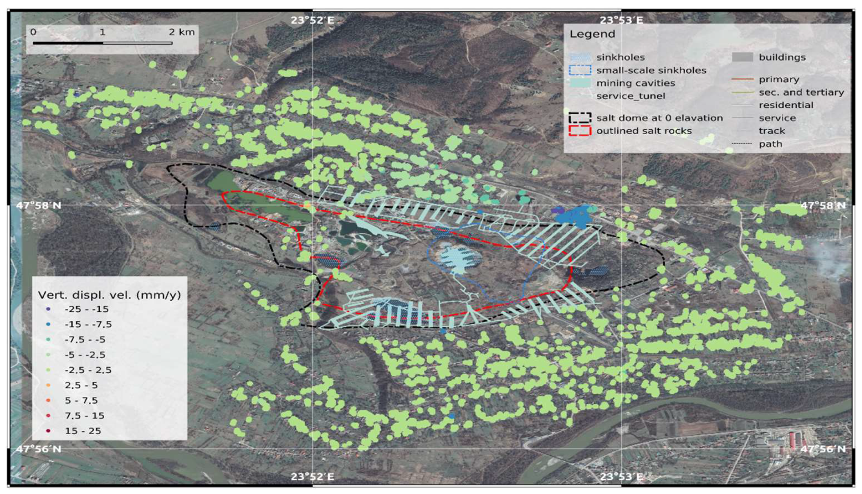
- To prepare a risk map for Solotvyno based on the results of interferometric processing and available auxiliary data sources.
2. Materials and Methods
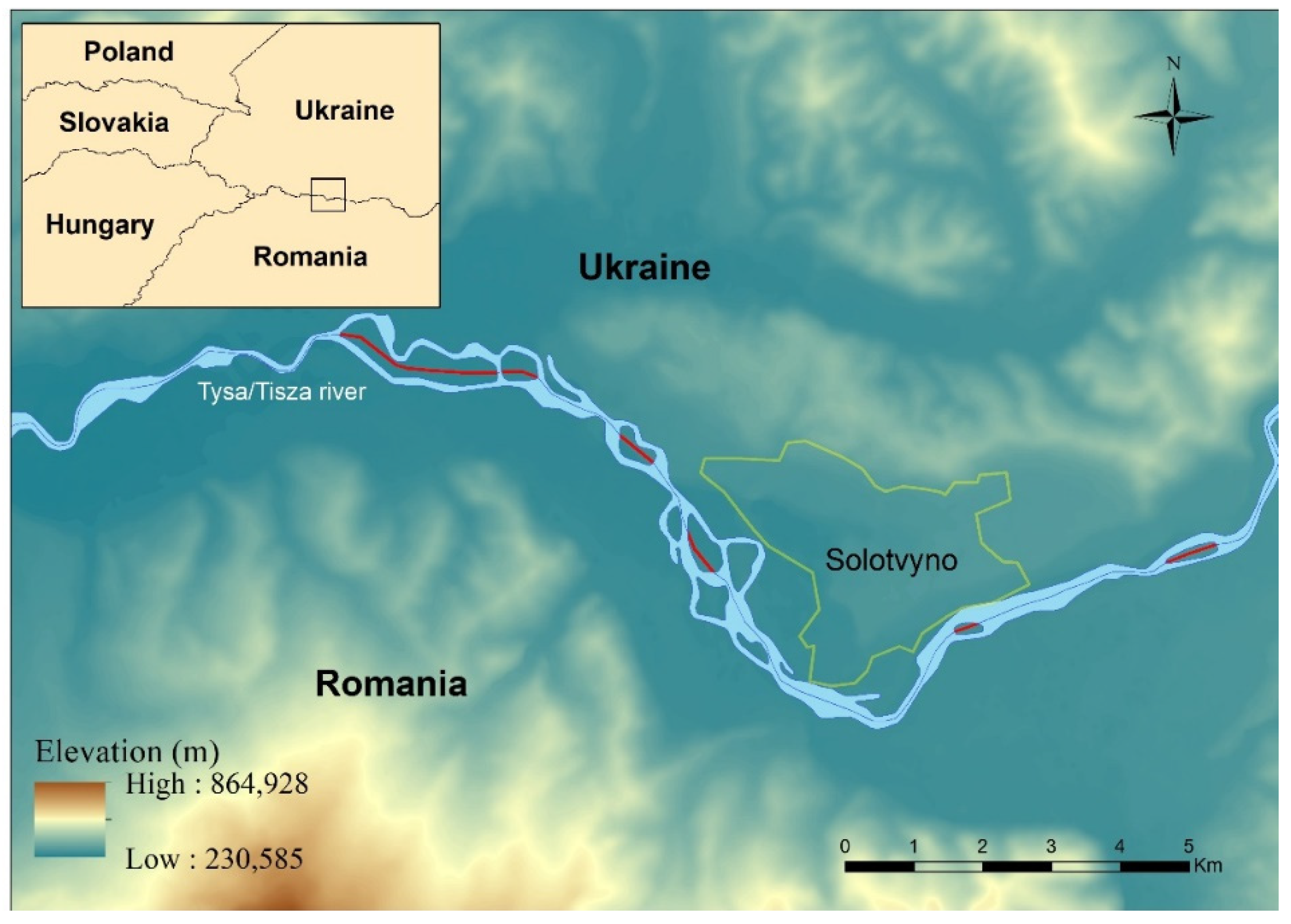
2.1. The Study Area
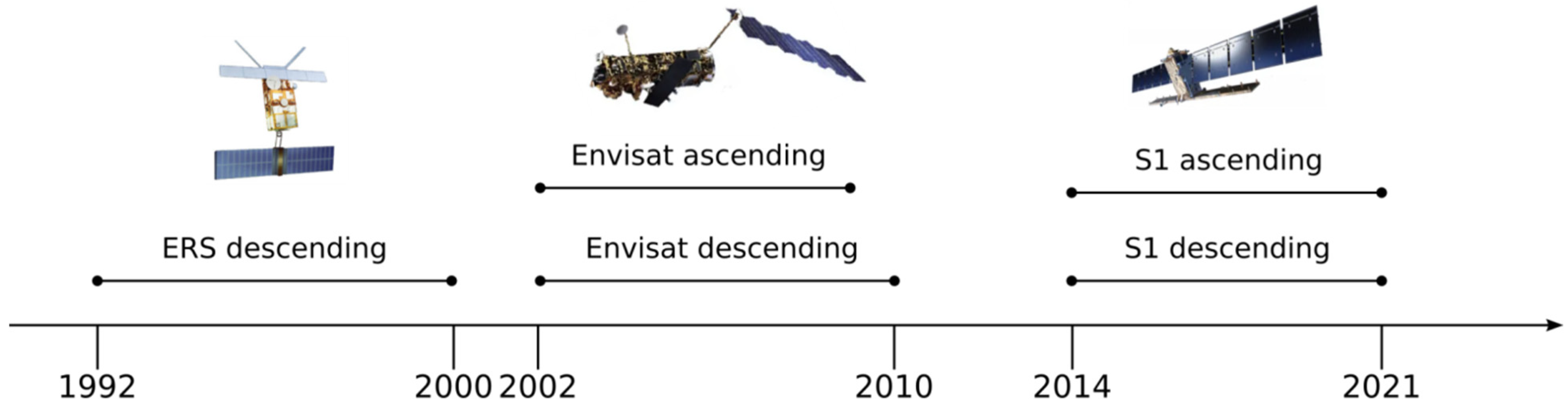
2.2. Satellite Data
2.3. Data-Processing Techniques
2.3.1. Interferometric Preprocessing
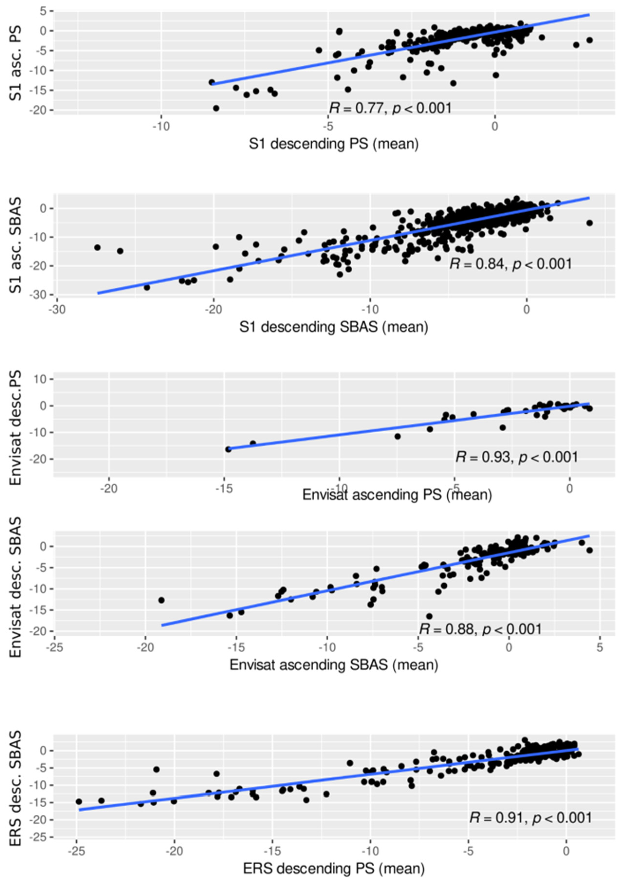
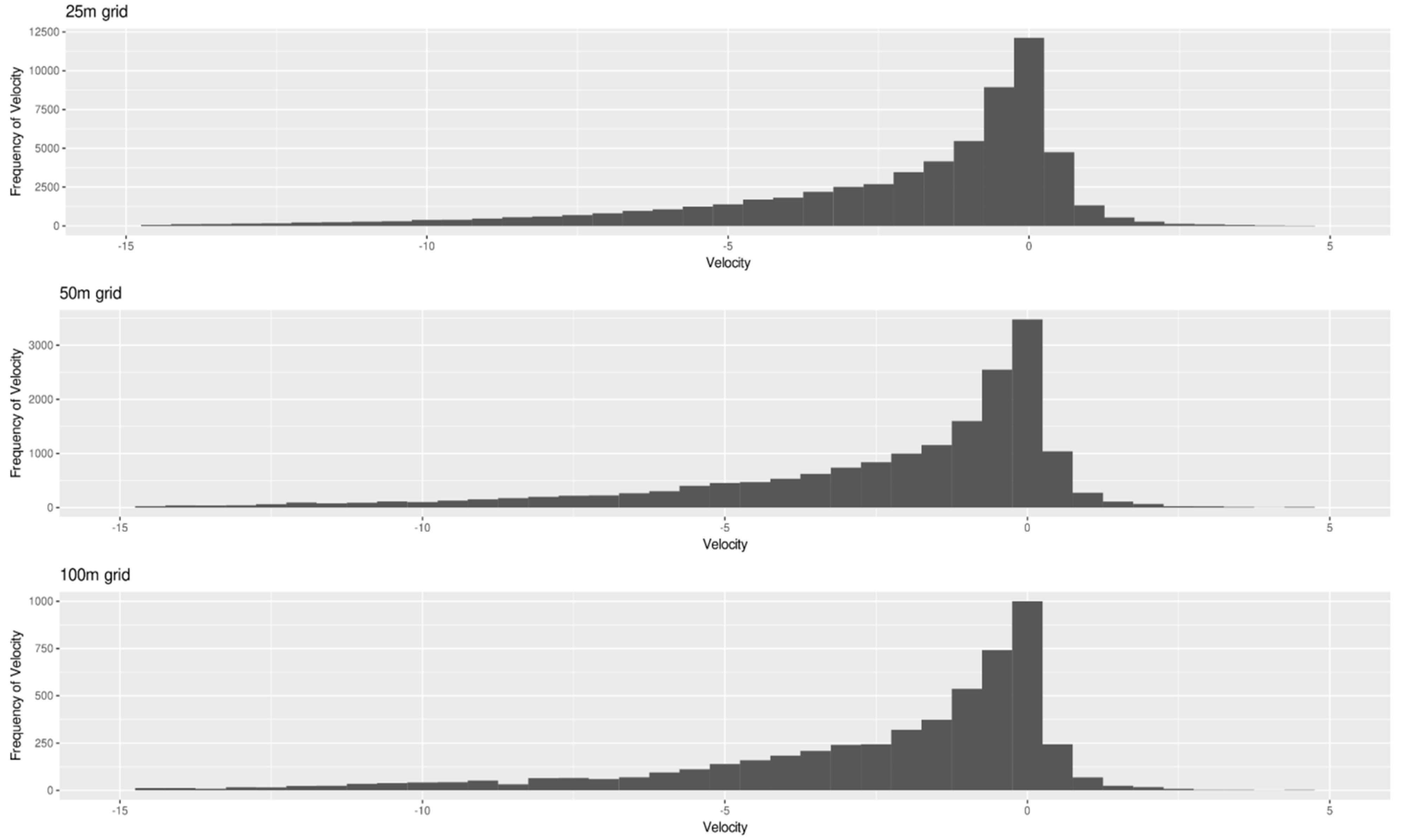
2.3.2. Data Fusion and Data Analysis
3. Results
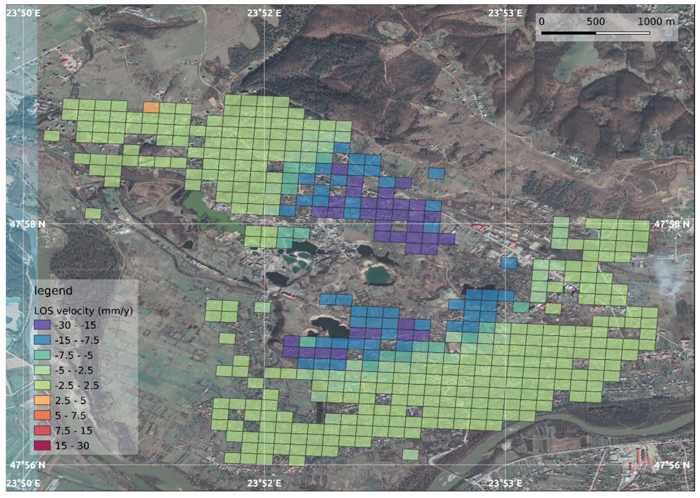
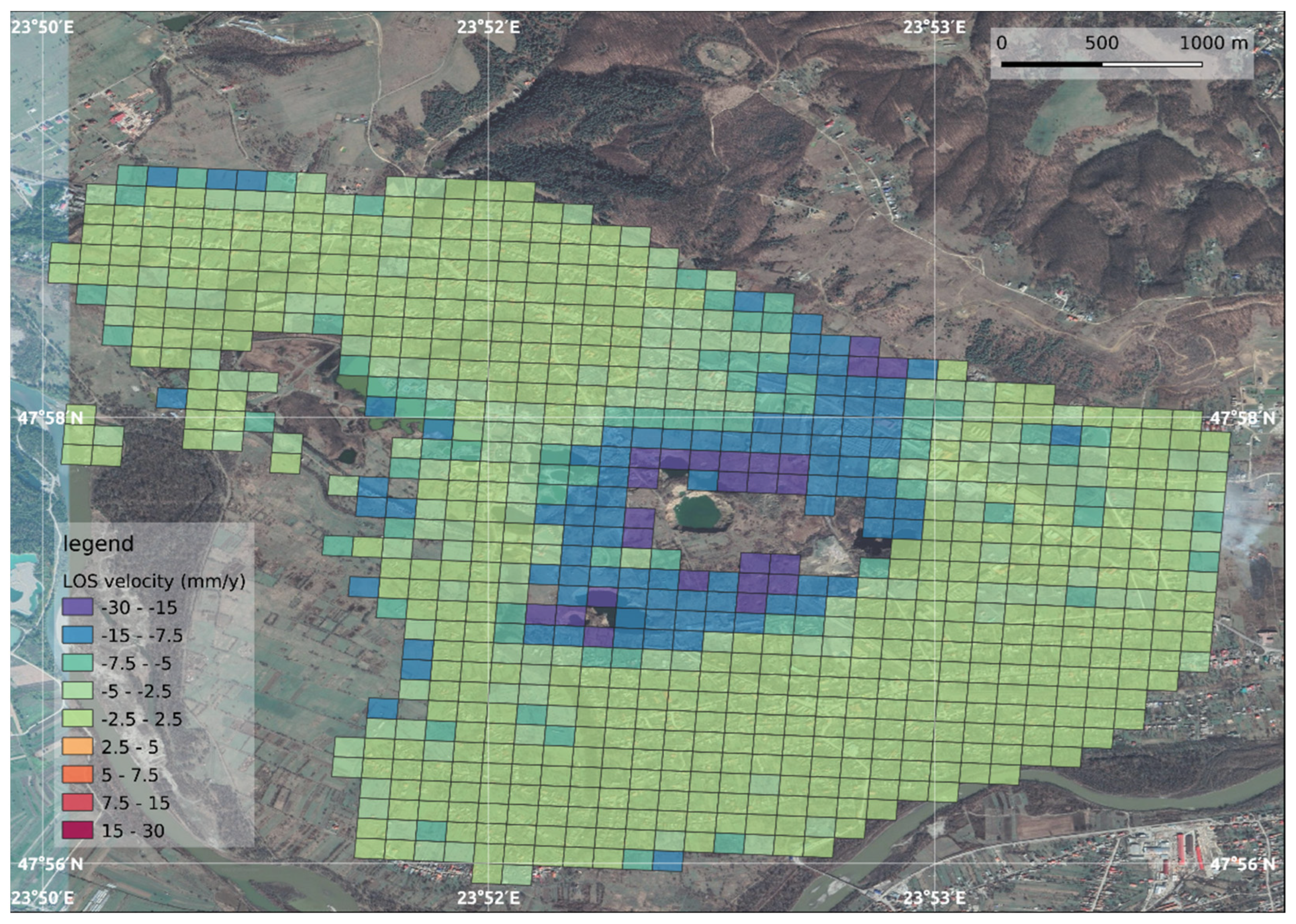
3.1. Interferometric Results (Annual Velocity of the Site According to Sensors)
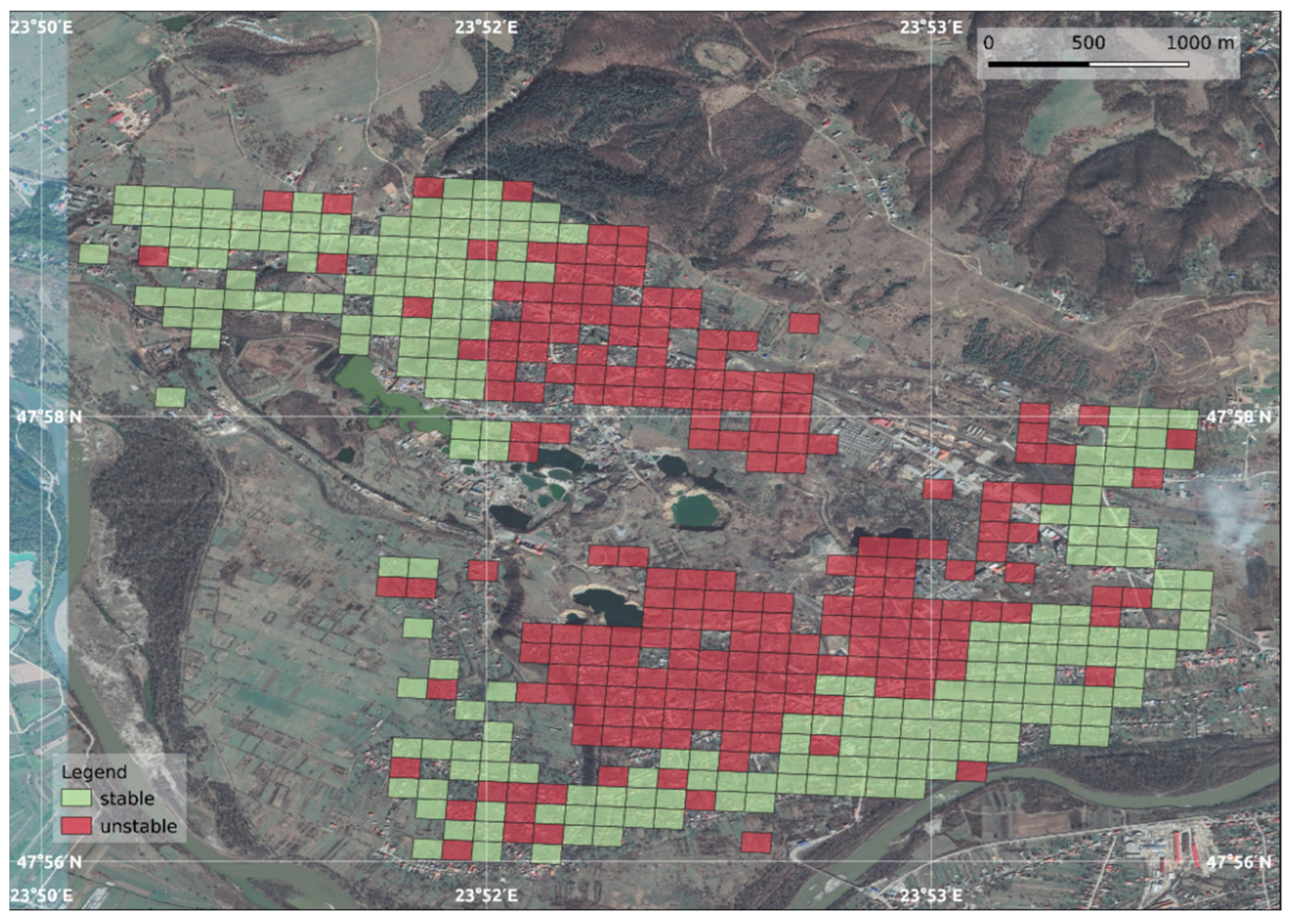
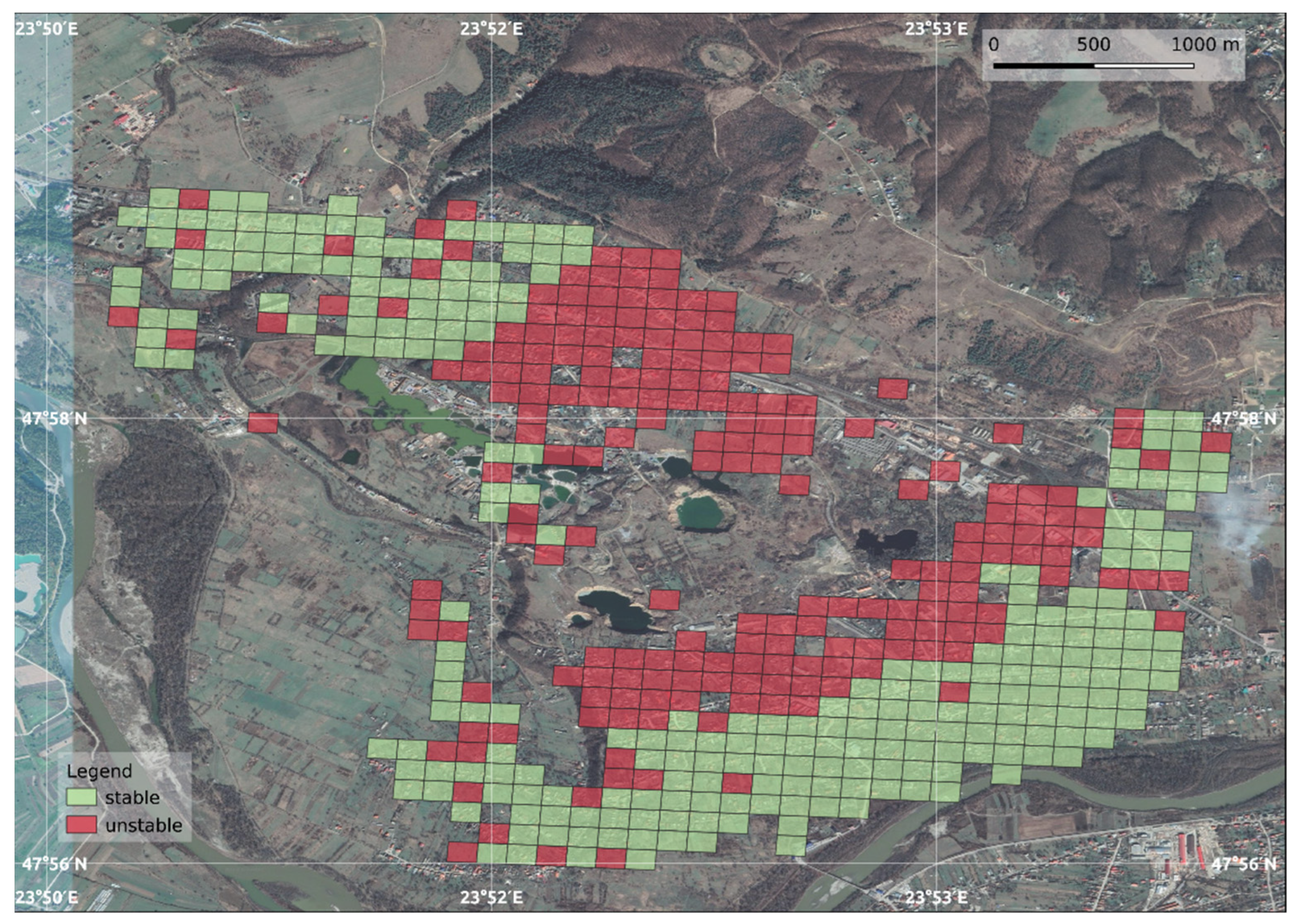
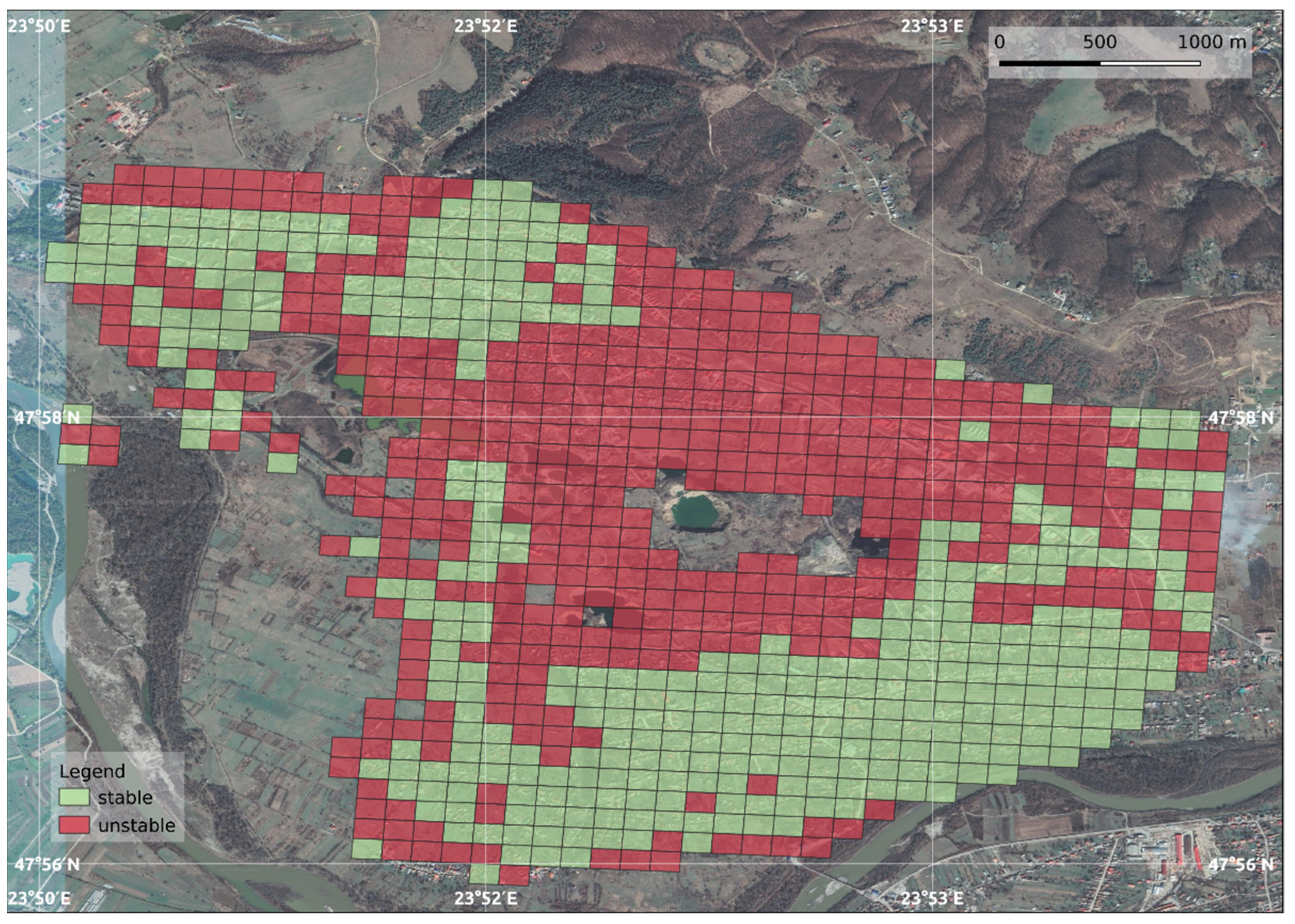
3.2. Stable Movement and Unstable Sites (According to Sensors)
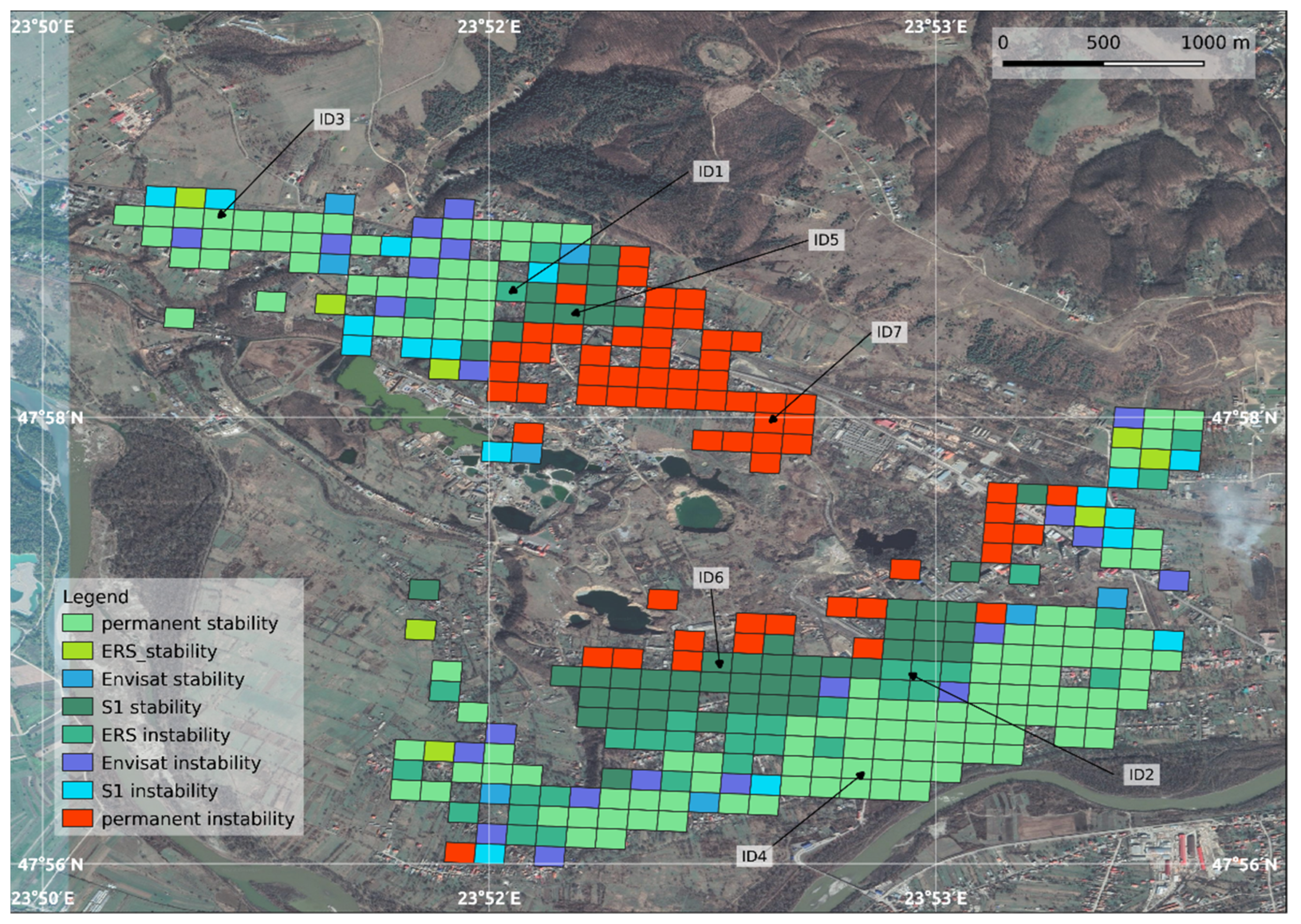
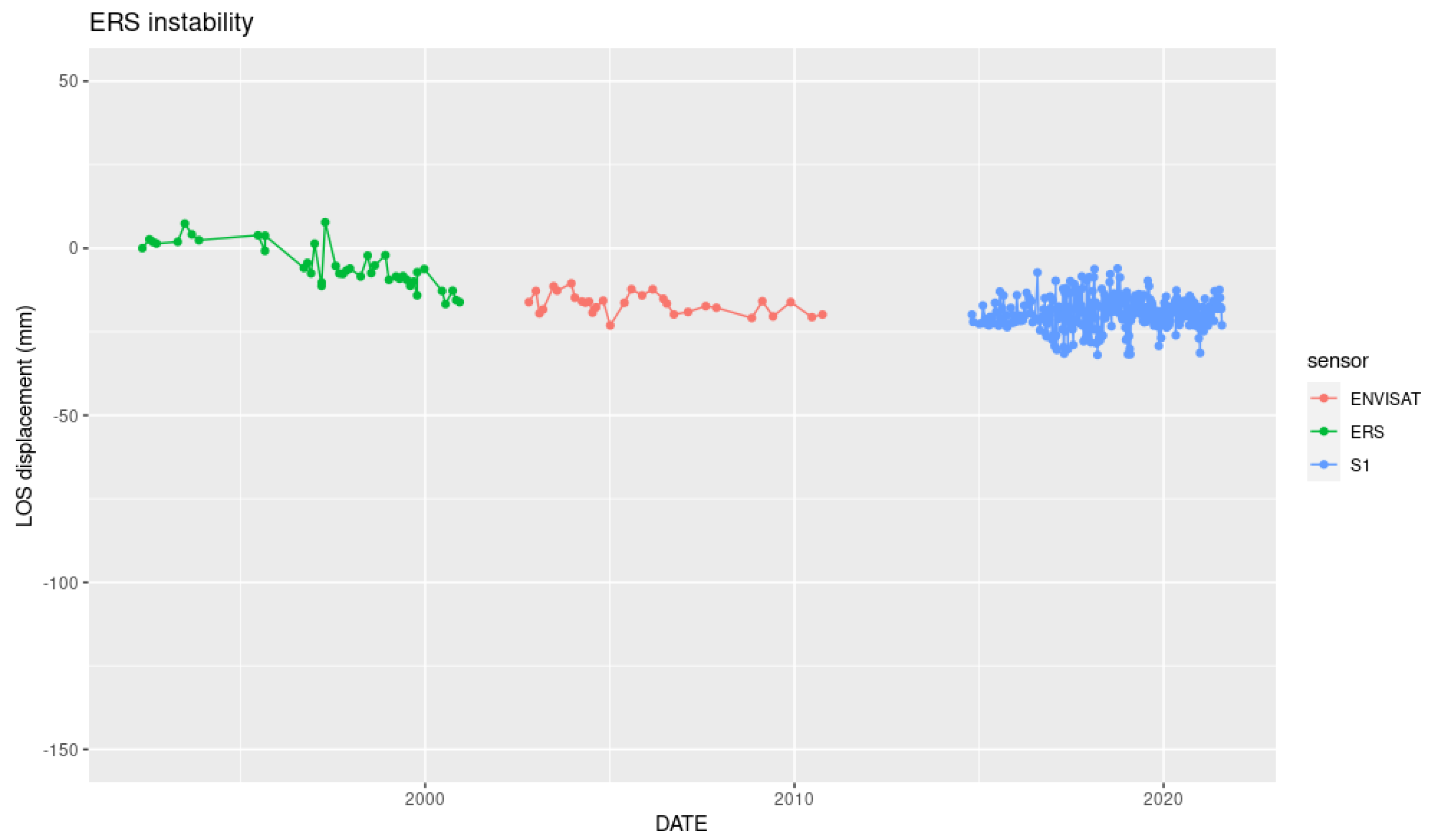
3.3. Multitemporal Changes of Stable and Unstable Sites and the Temporal Evolution of Unstable Sites
4. Discussion
5. Summary
Author Contributions
Funding
Institutional Review Board Statement
Informed Consent Statement
Data Availability Statement
Conflicts of Interest
References
- Herrero, C.; Catalina, J.C.; Muñoz, A. Prediction and Monitoring of Subsidence Hazards above Coal Mines (Presidence); European Commission: Brussels, Belgium, 2012. [Google Scholar] [CrossRef]
- Whyatt, J.; Varley, F. Catastrophic failures of underground evaporite mines. In Proceedings of the Twenty-Seventh International Conference on Ground Control in Mining, Morgantown, WV, USA, 29–31 July 2008; West Virginia University: Morgantown, WV, USA, 2008; pp. 113–122. [Google Scholar]
- Gourdier, S.; Bazargan-Sabet, B. Numerical Model for Assessment of Subsidence Due to Dissolution of Salt, Application to Nancy Basin (East of France). 2014. Available online: https://hal-brgm.archives-ouvertes.fr/hal-01025668 (accessed on 26 April 2022).
- Diao, X.; Wu, K.; Chen, R.; Yang, J. Identifying the Cause of Abnormal Building Damage in Mining Subsidence Areas using InSAR Technology. IEEE Access 2019, 7, 172296–172304. [Google Scholar] [CrossRef]
- Neal, J.T. Mine-Induced Sinkholes over the U.S. Strategic Petroleum Reserve (SPR) Storage Facility at Weeks Island, Louisiana: Geologic Mitigation and Environmental Monitoring. 1997. Available online: https://www.osti.gov/servlets/purl/459946 (accessed on 26 April 2022).
- Ege, J.R. Formation of Solution-Subsidence Sinkholes above Salt Beds; Geological Survey Circular 897; United States Department of the Interior: Washington, DC, USA, 1984.
- Szűcs, E.; Gönczy, S.; Bozsó, I.; Bányai, L.; Szakacs, A.; Szárnya Cs Wesztergom, V. Evolution of surface deformation related to salt-extraction-caused sinkholes in Solotvyno (Ukraine) revealed by Sentinel-1 radar interferometry. Nat. Hazards Earth Syst. Sci. 2021, 21, 977–993. [Google Scholar] [CrossRef]
- Delgado, J.M.P.Q.; Guimarães, A.S.; de Freitas, V.P.; Antepara i KoIí, V.; Herný, R. Salt Damage and Rising Damp Treatment in Building Structures. Adv. Mater. Sci. Eng. 2016, 2016, 1280894. [Google Scholar] [CrossRef] [Green Version]
- Móga, J.; Gönczi, S.; Berghauer, S.; Móga, K. Georesource or geohazard? Past, present and future of the salt mines in Solotvyno. GeoMetodika 2019, 3, 5–19. [Google Scholar] [CrossRef]
- Móga, J.; Lippman, L.; Tombor, E.; Fehér, K.; Kéri, A.; Borsodi, A. Geomorphological investigation of the Aknaszlatina saltkarst (Ukraine). Karsztfejlődés 2015, 20, 185–213. [Google Scholar]
- Móga, J.; Szabó, J.; Gönczy, S.; Lippmann, L.; Bódai, B. The study of the dynamically changing landforms of Aknaszlatina saltkarst by field and GIS methods. Karsztfejlődés 2017, 22, 139–161. [Google Scholar]
- Schuchová, K.; Lenart, J. Geomorphology of old and abandoned underground mines: Review and future challenges. Prog. Phys. Geogr. 2020, 44, 791–813. [Google Scholar] [CrossRef]
- Mancini, F.; Stecchi, F.; Stecchi, F.; Zanni, M.; Gabbianelli, G. Monitoring ground subsidence induced by salt mining in the city of Tuzla (Bosnia and Herzegovina). Environ. Geol. 2008, 58, 381–389. [Google Scholar] [CrossRef]
- Ray, R.L.; Lazzari, M.; Olutimehin, T. Remote Sensing Approaches and Related Techniques to Map and Study Landslides. In Landslides: Investigation and Monitoring; IntechOpen: London, UK, 2020; pp. 1–25. ISBN 978-1-78985-824-2. [Google Scholar] [CrossRef]
- Paradella, W.R.; Ferretti, A.; Mura, J.C.; Colombo, D.; Gama, F.F.; Tamburini, A.; Santos, A.R.; Novali, F.; Galo, M.; Camargo, P.O.; et al. Mapping surface deformation in open pit iron mines of Carajás Province (Amazon Region) using an integrated SAR analysis. Eng. Geol. 2015, 193, 61–78. [Google Scholar] [CrossRef] [Green Version]
- Berardino, P.; Fornaro, G.; Lanari, R.; Santosi, E. A New Algorithm for Surface Deformation Monitoring Based on Small Baseline Differential SAR Interferograms. IEEE Trans. Geosci. Remote Sens. 2002, 40, 2375–2383. [Google Scholar] [CrossRef] [Green Version]
- Ferretti, A.; Prati, C.; Rocca, F. Permanent scatterers in SAR interferometry. IEEE Trans. Geosci. Remote Sens. 2001, 39, 8–20. [Google Scholar] [CrossRef]
- Pasquali, P.; Cantone, A.; Riccardi, P.; Defilippi, M.; Ogushi, F.; Gagliano, S.; Tamura, M. Mapping of ground deformations with interferometric stacking techniques. In Land Applications of Radar Remote Sensing; Holecz, F., Pasquali, P., Milisavljevic, N., Eds.; InTechOpen: London, UK, 2014; pp. 231–258. [Google Scholar]
- Wasowski, J.; Bovenga, F.; Nutricato, R.; Conte, D.; Refice, A.; Kowalski, Z.; Graniczny, M. Satellite interferometry reveals spatial patterns of subsidence in the ancient Wieliczka salt mine (UNESCO heritage site, Poland). In Proceedings of the FRINGE 2007 Workshop, Frascati, Italy, 26–30 November 2007. [Google Scholar]
- Liu, X.; Xing, X.; Wen, D.; Chen, L.; Yuan, Z.; Liu, B.; Tan, J. Mining-Induced Time-Series Deformation Investigation Based on SBAS-InSAR Technique: A Case Study of Drilling Water Solution Rock Salt Mine. Sensors 2019, 19, 5511. [Google Scholar] [CrossRef] [PubMed] [Green Version]
- Kuzovenko, V.V. Geologic Map of Pre-Quaternary Formations; Transcarpathian Series L-34-XXXV (Uzhhorod), L-34-V (Satu Mare), Scale 1:200,000; Ministry of Ecology and Natural Resources of Ukraine: Kyiv, Ukraine; Department of Geology and Subsurface Use SGE “ZAKHIDUKRGEOLOGIYA”: Kyiv, Ukraine, 2001. (In Russian)
- Diakiv, V.; Bilonizhka, P. The characteristics of the geological structure and present day geoecological condition of Solotvyno salt bed. Bull. Lviv. Univ. Geol. 2010, 24, 62–79. [Google Scholar]
- Poklad, A. Ecological disaster in Solotvino. In Proceedings of the 16th International Scientific Conference Economics for Ecology (ISCS’2010), Sumy, Ukraine, 5–8 May 2010; pp. 120–122. [Google Scholar]
- Shekhunova, S.B.; Aleksieienkova, M.V.; Stadnichenko, S.M.; Siumar, N.P. The Integrated Geological Model of Solotvyno Structure as a Tool to Assess Geoecological Sustainability of Solotvyno Rocksalt Deposit. Collect. Sci. Work. Inst. Geol. Sci. NAS Ukr. 2015, 8, 233–250. [Google Scholar] [CrossRef]
- Velasco, V.; Sanchez, C.; Papoutsis, I.; Antoniadi, S.; Kontoes, C.; Aifantopoulou, D.; Paralykidis, S. Ground deformation mapping and monitoring of salt mines using InSAR technology. In Proceedings of the Solution Mining Research Institute Fall 2017 Technical Conference, Münster, Germany, 25–26 September 2017. [Google Scholar]
- Onencan, A.M.; Meesters, K.; Van de Walle, B. Methodology for Participatory GIS Risk Mapping and Citizen Science for Solotvyno Salt Mines. Remote Sens. 2018, 10, 1828. [Google Scholar] [CrossRef] [Green Version]
- Stoeckl, L.; Banks, V.; Shekhunova, S.B.; Yakovlev, Y. The hydrogeological situation after salt-mine collapses at Solotvyno, Ukraine. J. Hydrol. Reg. Stud. 2020, 30, 100701. [Google Scholar] [CrossRef]
- Yakovlev, E.O.; Shekhunova, S.B.; Aleksieienkova, M.V.; Siumar, N.P. Assessment of complex stress-strain of the Solotvyno salt anticline structure (basing on technique of natural pulse electromagnetic field of the Earth). Collect. Sci. Work. Inst. Geol. Sci. NAS Ukr. 2016, 9, 83–96. [Google Scholar] [CrossRef]
- ESA’s Online Dissemination Portal. Available online: https://esar-ds.eo.esa.int/oads/access/collection (accessed on 26 April 2022).
- Alaska Sar Facility. Available online: https://search.asf.alaska.edu/#/ (accessed on 26 April 2022).
- Jarvis, A.; Reuter, H.I.; Nelson, A.; Guevara, E. Hole-Filled SRTM for the Globe Version 4. 2008. Available online: http://srtm.csi.cgiar.org (accessed on 26 April 2022).
- Ng, A.H.M.; Ge, L.; Zhang, K.; Chang, H.C.; Li, X.; Rizos, C.; Omura, M. Deformation mapping in three dimensions for underground mining using InSAR–Southern highland coalfield in New South Wales, Australia. Int. J. Remote Sens. 2011, 32, 7227–7256. [Google Scholar] [CrossRef]
- Fialko, Y.; Simons, M. The complete (3-D) surface displacement in the epicentral area of the 1999 Mw 7.1 Hector Mine earthquake, California, from space geodetic observations. Geophys. Res. Lett. 2001, 28, 3063–3066. [Google Scholar] [CrossRef] [Green Version]
- Hanssen, R.F. Satellite radar interferometry for deformation monitoring: A priori assessment of feasibility and accuracy. Int. J. Appl. Earth Obs. 2005, 6, 253–260. [Google Scholar] [CrossRef]
- Colesanti, C.; Wasowski, J. Investigating landslides with space-borne Synthetic Aperture Radar (SAR) interferometry. Eng. Geol. 2006, 88, 173–199. [Google Scholar] [CrossRef]
- Casu, F.; Manzo, M.; Lanari, R. A quantitative assessment of the SBAS algorithm performance for surface deformation retrieval from DInSAR data. Remote Sens. Environ. 2006, 102, 195–210. [Google Scholar] [CrossRef]
- Crosetto, M.; Monserrat, O.; Iglesias, R.; Crippa, B. Persistent scatterer interferometry: Potential, limits and initial C- and X-band comparison. Photogramm. Eng. Remote Sens. 2010, 76, 1061–1069. [Google Scholar] [CrossRef]
- Cigna, F.; Bianchini, S.; Casagli, N. How to assess landslide activity and intensity with Persistent Scatterer Interferometry (PSI): The PSI-based matrix approach. Landslides 2013, 10, 267–283. [Google Scholar] [CrossRef] [Green Version]
- Pratesi, F.; Tapete, D.; Terenzi, G.; Del Ventisette, C.; Moretti, S. Rating health and stability of engineering structures via classification indexes of InSAR Persistent Scatterers. Int. J. Appl. Earth Obs. Geoinf. 2015, 40, 81–90. [Google Scholar] [CrossRef] [Green Version]
- Fiaschi, S.; Holohan, E.P.; Sheehy, M.; Floris, M. PS-InSAR Analysis of Sentinel-1 Data for Detecting Ground Motion in Temperate Oceanic Climate Zones: A Case Study in the Republic of Ireland. Remote Sens. 2019, 11, 348. [Google Scholar] [CrossRef] [Green Version]
- Kim, J.-W.; Lu, Z.; Degrandpre, K.; Kim, J.-W.; Lu, Z.; Degrandpre, K. Ongoing Deformation of Sinkholes in Wink, Texas, Observed by Time-Series Sentinel-1A SAR Interferometry (Preliminary Results). Remote Sens. 2016, 8, 313. [Google Scholar] [CrossRef] [Green Version]
- La Rosa, A.; Pagli, C.; Molli, G.; Casu, F.; De Luca, C.; Pieroni, A.; D’Amato Avanzi, G. Growth of a sinkhole in a seismic zone of the northern Apennines (Italy). Nat. Hazards Earth Syst. Sci. 2018, 18, 2355–2366. [Google Scholar] [CrossRef] [Green Version]


| Name of the Satellite and Geometry | Geometry | Start and End Dates of Acquisitions | Number of Images | Spatial Resolution (in meters) |
|---|---|---|---|---|
| ERS | descending | May 1992–December 2000 | 42 | 25 |
| Envisat | ascending | October 2002–August 2009 | 25 | |
| Envisat | descending | October 2002–October 2010 | 31 | |
| Sentinel-1 | ascending | October 2014–October 2021 | 341 | 15 |
| Sentinel-1 | descending | October 2014–October 2021 | 337 | 15 |
| Terminology | Definition | Stability and Instability during Acquisitions | ||
|---|---|---|---|---|
| ERS (1990s) | Envisat (2000s) | S1 (2014–2021) | ||
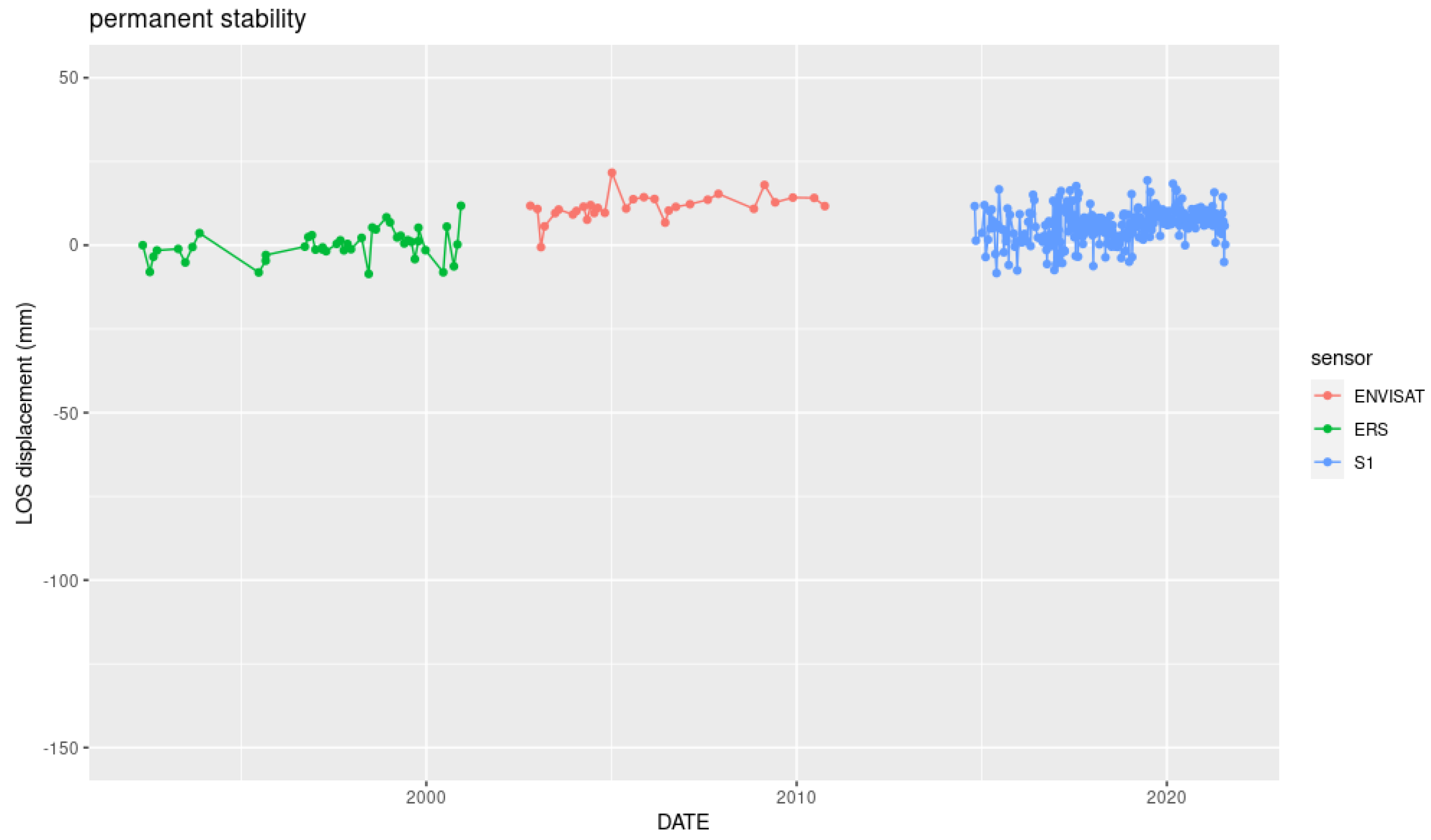
| permanent stability | The grid was stable over the last 30 years. | ⊕ | ⊕ | ⊕ |
| permanent instability | The grid was unstable over the last 30 years. | ⊖ | ⊖ | ⊖ |
| ERS stability | The grid was stable during ERS acquisitions and became unstable. | ⊕ | ⊖ | ⊖ |
| Envisat stability | The grid was unstable during ERS acquisitions, became stable during Envisat acquisitions, and became unstable again. | ⊖ | ⊕ | ⊖ |
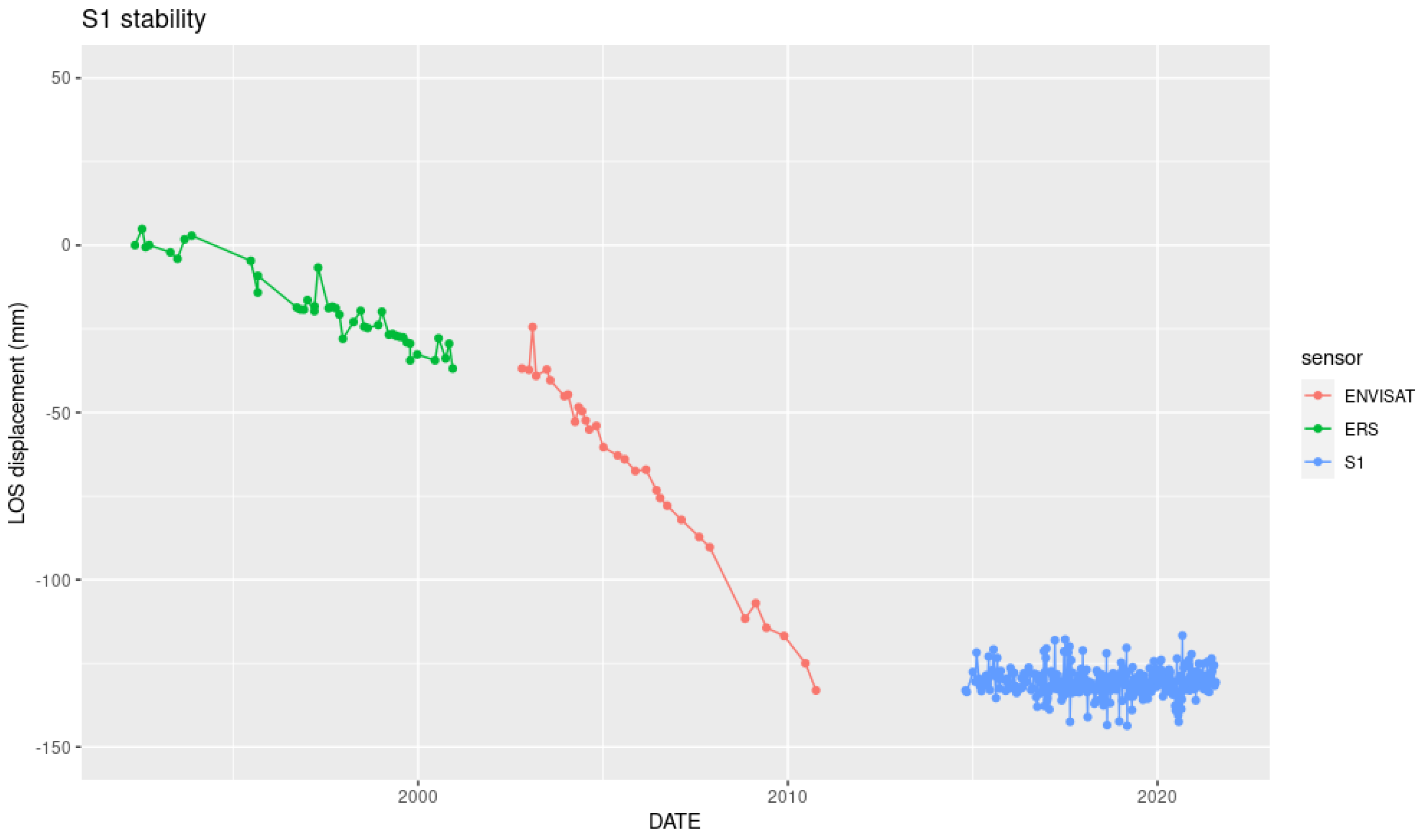
| S1 stability | The grid was permanently instable during ERS and Envisat but stable during S1 acquisitions. | ⊖ | ⊖ | ⊕ |
| ERS instability | The grid was instable during ERS but became stable on later acquisitions. | ⊖ | ⊕ | ⊕ |
| Envisat instability | Instability occurred during Envisat acquisitions. | ⊕ | ⊖ | ⊕ |
| S1 instability | The grid was permanently stable during ERS and Envisat but destabilized during S1 acquisitions. | ⊕ | ⊕ | ⊖ |
Publisher’s Note: MDPI stays neutral with regard to jurisdictional claims in published maps and institutional affiliations. |
© 2022 by the authors. Licensee MDPI, Basel, Switzerland. This article is an open access article distributed under the terms and conditions of the Creative Commons Attribution (CC BY) license (https://creativecommons.org/licenses/by/4.0/).
Share and Cite
Dobos, E.; Kovács, I.P.; Kovács, D.M.; Ronczyk, L.; Szűcs, P.; Perger, L.; Mikita, V. Surface Deformation Monitoring and Risk Mapping in the Surroundings of the Solotvyno Salt Mine (Ukraine) between 1992 and 2021. Sustainability 2022, 14, 7531. https://doi.org/10.3390/su14137531
Dobos E, Kovács IP, Kovács DM, Ronczyk L, Szűcs P, Perger L, Mikita V. Surface Deformation Monitoring and Risk Mapping in the Surroundings of the Solotvyno Salt Mine (Ukraine) between 1992 and 2021. Sustainability. 2022; 14(13):7531. https://doi.org/10.3390/su14137531
Chicago/Turabian StyleDobos, Endre, István Péter Kovács, Dániel Márton Kovács, Levente Ronczyk, Péter Szűcs, László Perger, and Viktória Mikita. 2022. "Surface Deformation Monitoring and Risk Mapping in the Surroundings of the Solotvyno Salt Mine (Ukraine) between 1992 and 2021" Sustainability 14, no. 13: 7531. https://doi.org/10.3390/su14137531
APA StyleDobos, E., Kovács, I. P., Kovács, D. M., Ronczyk, L., Szűcs, P., Perger, L., & Mikita, V. (2022). Surface Deformation Monitoring and Risk Mapping in the Surroundings of the Solotvyno Salt Mine (Ukraine) between 1992 and 2021. Sustainability, 14(13), 7531. https://doi.org/10.3390/su14137531