Combined PV-Wind Hosting Capacity Enhancement of a Hybrid AC/DC Distribution Network Using Reactive Control of Convertors and Demand Flexibility

Abstract

The integration of Renewable Energy Sources (RESs) into distribution networks has increased in recent years due to numerous advantages. However, the RESs are intermittent and uncertain therefore may cause various limitations such as high lines loading and large voltage deviations, especially during high generation and low demand periods. Thus, this leads to an upper limit for the integrated capacity of RESs into the network, entitled Hosting Capacity (HC). In this paper, the complementarity of wind-PV along with the Demand Flexibility Program (DFP) are utilized for alleviating the limitations and increasing the HC in a hybrid AC/DC network. Moreover, an important feature of the AC/DC network, i.e., reactive control of Voltage Source Converters (VSCs) is investigated for increasing the HC. Additionally, a tradeoff is made between two conflicting objectives, i.e., HC and energy losses, which will be increased due to an excessive increase of the HC. Generally speaking, the paper proposes a multi-objective, multi-source, and multi-period extended optimal linear power flow model for simultaneously increasing the HC and decreasing the energy losses, utilizing stochastic programming for managing uncertainties. The simulation results show the accuracy and efficiency of the proposed formulation from various perspectives.

1. Introduction

1.1. Motivation

Hosting Capacity (HC) is known as the capacity of a distribution network for accepting the DG units, especially the renewable types such as Wind Turbine (WT) and solar PV, without violating any network limitation. An increase in Renewable Energy Sources (RESs) has some positive and negative effects on the Distribution Network Operator/Owner (DNO) [1]. Reducing greenhouse gas emissions and postponing the need for network reinforcement are some of the positive effects of using RESs. However, some obstacles may hold back the penetration increase of these sources. For example, the intermittent nature of RESs [2] and their dependency on environmental parameters such as wind speed, ambient temperature, and solar radiation [3] are some of the negative features. Specifically speaking, high generation of RESs in the distribution network, may lead to overvoltage and overflow issues due to the reverse power flow phenomenon. Such issues and their effect on the HC of the distribution networks are of great importance, especially for the arising concept of hybrid AC/DC networks.

Besides this, both DNO and Distribution Generator Owners (DGOs) are interested in an increase of Distributed Generations (DGs) capacity. However, this may intensify the network energy loss, which is not favorable from the DNO’s perspective. Therefore, other objectives such as energy losses must be considered as well, when optimizing the HC. In addition, the advent of Demand Response (DR) concepts [4] delivers flexibility for DNO to achieve these contradictory goals. In addition, the reactive power control of Voltage Source Converters (VSCs), connecting the AC and DC parts of the hybrid networks, can be used for these purposes. Based on the above explanations, this paper proposes a linear stochastic model for maximizing the combined PV-WT HC while minimizing the energy losses for a hybrid AC/DC network using the potentials of the Demand Flexibility Program (DFP) and the reactive power control of VSCs (QSVC) as an Active Network Management (ANM) scheme.

1.2. Literature Review

Integrating the DGs into the network is one of the most important challenges of the future power system. Since most of the distribution networks are radial, the presence of DG units was not considered at their design stage [5]. However, incentivization and simplification of the access to the network caused an increase in the penetration rate of small DGs into the network. Nevertheless, several problems have been reported limiting the DGs HC, such as overvoltage, thermal limits of lines [6], protection malfunction, and power quality issues [7,8]. It should be noted that the limitation of various constraints such as voltage rise and power flow through the lines usually occurs at the maximum generation and minimum demand due to the highest reverse power flow and voltage increase in these periods.

Many studies have focused on increasing the HC with different methods considering some of the abovementioned limitations. For example, some studies have increased the HC of dispatchable DGs using optimal sizing and sitting [9] and optimal network reconfiguration [10] considering voltage and thermal limits. However, DGs based on RESs are mainly non-dispatchable and this can make the HC problem more complicated. Nevertheless, using this type of DG is constantly increasing due to environmental concerns and the need for de-carbonization. Therefore, the variable and uncertain outputs of RESs-based DGs should be considered in determining the HC.

Using various ANM schemes is one of the possible approaches for handling the variability of RESs and increasing the HC. ANM schemes mainly organize the connection between DGs and network equipment using various control mechanisms to facilitate a larger output from the DGs [11]. Voltage control via Under-Load Tap Changer (ULTC) transformers [12], voltage regulators [13], active management strategies such as DGs active power curtailment [14], network reconfiguration [15,16], and energy storage [17] are some of the ANM schemes used for the HC enhancement. Most of the studies either consider one type of RESs or do not examine the effect of combining them for the HC improvement. Additionally, reactive power control strategies are included as an ANM scheme, which is applied in various studies for HC enhancement. Reactive power control of inverters in DGs [6], smart inverters, i.e., STATCOM, considering both dynamic and static HC [18], Volt/VAr control process of electric vehicles [19], and capacitor bank [20] are the HC enhancement studies, which consider reactive power control strategies. However, the new ANM potentials of hybrid AC/DC distribution networks, such as reactive power control of the VSCs, are not utilized for HC purposes.

Another approach to ease meeting the limitations of RESs variability is to use the complementarity between various RESs [21], i.e., two or more energy sources with complementary availability periods such as PV and WT [11]. Many studies have reported the merits of complementarity of various RESs in various countries such as Italy [22] and Canada [23]. Even though Hybrid Renewable Energy Sources (HRESs) can be used to mitigate the RESs intermittency, it requires careful consideration for selecting the deployment sites and the shares of RESs types in the designing stage [24].

According to the literature, few studies have been done on the HC assessment and enhancement based on HRESs. In [25], a stochastic framework is developed to study the hybrid PV-WT system HC. However, in this study, the potentials of DFP and ANM schemes for increasing the HC have not been considered, and the negative effect on the energy losses is ignored. In [11], an optimal power flow method is developed to configure WT and PV capacity for maximizing energy generation while obligating to the network limits. In this study, the simultaneous effect of some ANM schemes and HRES is demonstrated on the HC based on multiple location deployment. Nevertheless, the DFP potentials and the effect of HC increase on the energy losses are not investigated. Besides the above-mentioned limitations, almost all these studies are single locations, and there are few works considering the network-wide influence of HRES in multiple locations. In addition, an economic evaluation between single location and multiple locations deployment of RESs in the hybrid AC/DC distribution network has been undertaken.

As mentioned earlier, an increase in the HC usually increases the energy losses. Most of the studies examining the impact of RESs on the HC have neglected the energy losses issue. DR programs, in the context of DFP, can reduce the reverse power flow of the lines and overcomes the constraints imposed by RESs. Therefore, DFP causes a simultaneous increase in the HC and a decrease in the energy losses. Reference [26] deals with the effect of DFP on HC in terms of energy losses in the form of a multi-objective nonlinear programming model. Reference [27] examines different ANM schemes on HC enhancement considering DFP based on a mixed-integer second-order cone programming model in which the optimization of energy losses is neglected. These studies only consider the WT or PV (non-HRES) and the AC network (non-hybrid) and neglect the RESs uncertainty.

On the other hand, the capacity of the network may not be fully utilized due to the variability of the RESs. Connecting two feeders and operating the AC network as a meshed grid, can reduce the lines loading and improve the voltage profile, thereby, enhancing the HC [28]. However, the AC distribution network operates radially and the creation of a mesh in it leads to destructive circulating currents [29]. One solution is to use the concept of hybrid AC/DC distribution networks and connect the two parts of the network by VSCs. The various benefits of using DC power alongside the AC have been demonstrated in numerous studies. Reference [30] has shown that the use of DC power in the distribution network has enhanced the voltage profile and the power transfer of the network feeders. In [31], the use of DC power has reduced the network losses compared to the fully AC network. According to the literature review, as far as the authors are aware, all the studies focusing on the HC issue have been developed for the AC distribution network, and the potentials of the hybrid AC/DC networks are neglected.

This paper aims to address all of the above issues. Therefore, the effects of HRESs (PV-WT) along with DFP are considered for increasing the HC and reducing the energy losses at the same time. The proposed model is presented as multi-source, multi-objective, and multi-period stochastic (considering the uncertainties) linear programming. Developing the model for a hybrid AC/DC distribution network helps to increase the HC and decrease the energy losses by combining the advantages of the two types of network and the reactive power control of the VSCs as an ANM scheme.

Table 1. Summary of existing studies and contribution of the present paper.

	MILP Model	Multi Objectives Framework	Hybrid RESs	RESs Uncertainty	Stochastic Model	Hybrid AC/DC Network	Tools
							DFP	ANM (QVSC)	ANM (Others)
[6]	✘	✓	✘	✓	✓	✘	✘	✘	✓
[11]	✘	✘	✓	✘	✘	✘	✘	✘	✓
[12]	✘	✘	✘	✓	✓	✘	✘	✘	✓
[13]	✓	✓	✘	✘	✘	✘	✘	✘	✓
[14]	✘	✘	✘	✘	✘	✘	✘	✘	✓
[15]	✘	✓	✘	✓	✘	✘	✘	✘	✓
[16]	✓	✓	✘	✓	✓	✘	✘	✘	✓
[17]	✘	✓	✘	✘	✘	✘	✘	✘	✓
[19]	✘	✘	✘	✘	✘	✘	✘	✘	✓
[20]	✘	✘	✘	✘	✘	✘	✘	✘	✓
[25]	✘	✘	✓	✓	✘	✘	✘	✘	✓
[26]	✘	✓	✘	✘	✘	✘	✓	✘	✓
[27]	✘	✘	✘	✘	✘	✘	✓	✘	✓
Current paper	✓	✓	✓	✓	✓	✓	✓	✓	✓

✓/✘ denotes that the subject is/is not considered.

reviews some recent studies regarding the above-mentioned perspectives. This table also presents the novelties of the current work compared to the most related studies in the field.

1.3. Contributions and Organization

According to the challenges and research gaps discussed earlier, this paper addresses a multi-objective, multi-source, and multi-period stochastic optimal linear power flow-based assessment approach for the optimal sizing and location of HRES in a hybrid AC/DC distribution network in order to increase the HC and reduce the energy losses considering the DFP and ANM.

Therefore, the contributions and features of this paper are as follows:

• Proposing a stochastic and linearized model for the HC problem of HRES (PV-WT) (sizing in multi-candidate locations) in the hybrid AC/DC distribution network.
• Utilizing the reactive power control of VSCs (QSVC) as an ANM scheme for increasing the HC and reducing the network energy losses.
• Including the DFP in the proposed formulation in order to achieve the objectives of the problem.
• Presenting a multi-objective, multi-source, and multi-period optimization framework (increasing HC and reducing energy losses) based on ɛ-constraint and fuzzy satisfying methods.

The rest of the paper is organized as follows. Section 2 describes the structure of the AC/DC hybrid distribution network. In Section 3, uncertainty modeling is discussed. In Section 4, the multi-objective stochastic optimization problem is formulated. Section 5 presents the simulation results. Finally, the paper is concluded in Section 6.

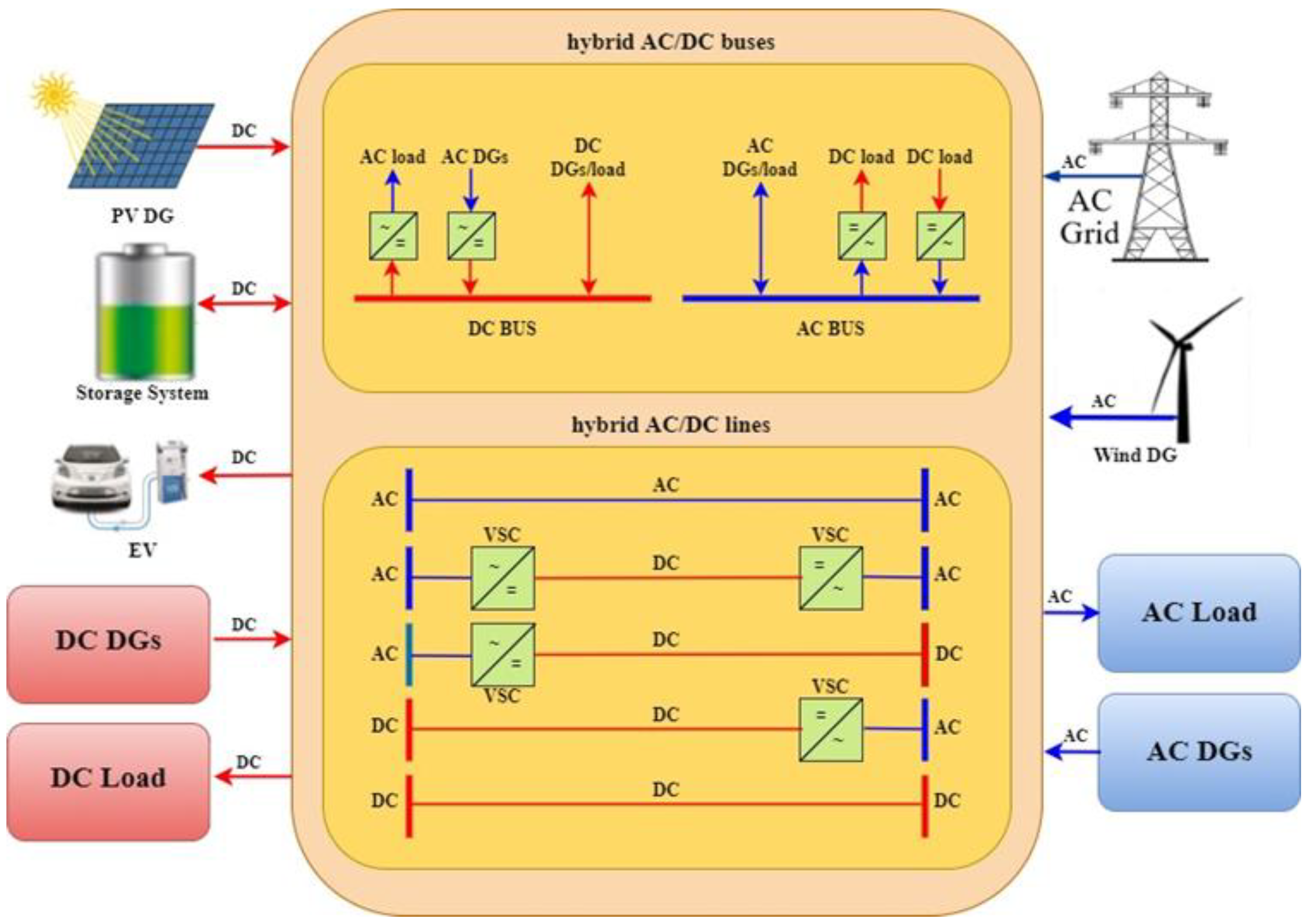
2. Structure of a Hybrid AC/DC Distribution Network

The future smart distribution network will include a variety of AC and DC loads and DGs. Examples of DC DGs are solar PV and fuel cells. Modern elevators, electric vehicles, and industrial loads are also examples of DC loads. For an optimal adaptation of this type of loads and DGs, the current belief is that the distribution network should be of a hybrid type [32] that includes AC/DC buses, lines, and converters, as depicted in Figure 1. This figure shows the hybrid AC/DC distribution network buses and lines, as well as the connection of loads, DGs, and storages [33] to the AC and DC buses. AC/DC interface converters in the network are essential for (1) connecting DC loads and DC DGs to the AC buses, (2) connecting AC loads and AC DGs to the DC buses, and (3) connecting the DC and AC parts of the network together. In this paper, VSCs are used in the hybrid distribution network in order to exchange active AC and DC powers and also control the injected/received reactive power to the AC distribution network. It is worth noting that in a smart hybrid AC/DC grid, a bi-directional communication system is also needed for (1) collecting all the information and measurements from the network and transferring them to the DNO, and (2) transferring optimal decisions of the DNO to the various equipment of the network.

3. Uncertainty Modeling

3.1. Modeling of RESs Uncertainty

The output power of RESs depends on the weather conditions and inherently has many variabilities and uncertainty. This leads to an upper limit for these sources’ capacity to integrate into the distribution network. Therefore, the uncertainty of these sources should be considered in the HC problem. In this paper, due to the focus on the HRESs, there are two main sources of uncertainty, PV and WT. The uncertainty of these RESs is considered in the model and the problem is developed as a scenario-driven optimal stochastic model. In such cases, where a set of scenarios needs to be handled, the main issue is to generate a realistic list of scenarios for the random variables illustrating the possible properties of the data properly. The initial set of scenarios is a large dataset generated by the Monte Carlo simulation (MCS) method, representing the uncertainties. The MCS parameters are Probability Distribution Functions (PDFs) of the forecast errors obtained from the historical data. To consider the forecast error, a positive or negative term is added to the forecasted value ($X^{forecast}$), as presented in (1) [34].

$$\begin{array}{cc}{X}^s(t)=X^{forecast}(t)+X^{error,s}(t)& \forall t,\forall s\end{array}$$

(1)

In this equation, the error term ($X^{error, s}$) is a zero-mean noise with a standard deviation ($\sigma$), and the values of parameters in various scenarios are presented by $X^s$. In this paper, the forecast errors for all of the uncertain parameters are included based on the normal PDFs.

Including all of the generated scenarios into the optimization, results in a large-scale problem. Generally, there should be a trade-off between model accuracy and computation speed. In this paper, a standard scenario reduction method developed in [34] is utilized to overcome the problem of the high computational burden. The recommended scenario reduction procedure has three algorithms with different accuracies, i.e., fast-backward method, fast backward/forward method, and fast-backward/backward method. Choosing the appropriate algorithm is subject to the size of the under-investigation problem and the desired solution precision. In this paper, the fast-backward technique is selected to achieve the best computational performance. This algorithm eliminates the low probability scenarios and merges those that are close to each other. Subsequently, the solutions could be found more efficiently without downgrading the final accuracy by maintaining the most important statistical characteristics of the original dataset.

3.2. Two-Stage Stochastic Optimization Modeling

The two-stage stochastic programming method is used for decision-making under the uncertainties in this paper. Further details on the stochastic programming method can be found in [35]. In this method, the decision variables are divided into two categories, i.e., “here and now” and “wait and see”. Since the “first stage” or “here and now” variables are independent of the scenarios, their optimal values must be determined before the scenario’s realization. On the other hand, the optimal value of the “second stage” or “wait and see” variables must be determined when the scenarios are realized. This is because they may have different values in different scenarios. The set of “here and now” ($D_{HN}$) and “wait and see” ($D_{WS}$) variables are presented in (2) and (3), respectively.

$$D_{HN}=\left\{\begin{array}{ccc}{C}_i^{w,ac}& ,& i\in {\mathsf{\Omega }}_w^{ac}\\ C_i^{pv,ac}& ,& i\in {\mathsf{\Omega }}_{pv}^{ac}\\ C_{id}^{w,dc}& ,& id\in {\mathsf{\Omega }}_w^{dc}\\ C_{id}^{pv,dc}& ,& id\in {\mathsf{\Omega }}_{pv}^{dc}\end{array}\right\}$$

(2)

$$D_{WS}=\left\{V_{i,t,s}^{ac},V_{id,t,s}^{dc},{\theta }_{ij,t,s},P_{i,t,s}^{(w,pv),ac},P_{id,t,s}^{(w,pv),dc},P_{i,t,s}^{(cw,cpv),ac},P_{id,t,s}^{(cw,cpv),dc},P_{i,t,s}^{sb},P_{i,t,s}^{cvtac},P_{id,t,s}^{cvtdc},Q_{i,t,s}^{(w,pv),ac},Q_{id,t,s}^{(w,pv),dc},Q_{i,t,s}^{sb},Q_{i,t,s}^{cvtac}\right\}$$

(3)

The variables in (2) are related to the installed capacity of WT and PV sources in both AC and DC distribution networks. These variables are independent of the scenarios. The variables in (3) are related to the active/reactive power of RESs, RESs’ power curtailment, the active/reactive power of VSCs, the active/reactive power of upstream grids, and AC and DC distribution networks, voltages, which depend on the scenarios.

4. Problem Formulation

In this section, the proposed model is formulated as a stochastic Mixed Integer Linear Programming (MILP) optimization problem. After describing the objective functions (HC and energy losses), the constraints related to the power flow equations of AC and DC distribution networks are introduced. Then, the model of DFP in both networks and the VSCs model with its constraints are presented. After that, the linearization of the problem is discussed. Additionally, the multi-objective optimization framework based on the ɛ-constraint and fuzzy satisfying methods is explained. Finally, the solution procedure is described.

4.1. Objective Functions

The objective functions of the problem are considered as presented in (4) and (5): ($\forall i\in \{{\Omega }_w^{ac},{\Omega }_{pv}^{ac}\}$, $\forall id\in \{{\Omega }_w^{dc},{\Omega }_{pv}^{dc}\}$, $\forall i\in {\Omega }_{cvt }^{ac}$, $\forall t\in {\mathsf{\Omega }}_T$, $\forall s\in {\mathsf{\Omega }}_S$).

$$max\left\{F_1\right\}=max\{F_1=\sum _i(C_i^{w ,ac}+C_i^{pv ,ac})+\sum _{id}(C_i^{w ,dc}+C_i^{pv ,dc})\}$$

(4)

$$min\left\{F_2\right\}=min\{F_2=(\sum _{t ,s}{Ploss}_{t ,s}^{ac}+\sum _{t ,s}{Ploss}_{t ,s}^{dc}+\sum _i\sum _{t ,s}{Ploss}_{i ,t ,s}^{cvt})\ast {\pi }_s\ast {\tau }_d\}$$

(5)

Equation (4) shows the HC of the hybrid AC/DC distribution network and (5) refers to the energy losses. The first and second terms of (4) are related to the installed capacity of WT and PV sources in AC and DC distribution networks, respectively. Total network energy losses ($F_2$) within a one-year time span are calculated based on the summation of the AC and DC distribution network losses (details are presented in (6) and (27), respectively) and the VSC losses (details are presented in (52)) at all hours (t) and all scenarios (s) multiplied by the probability of scenarios (${\pi }_s$) and the number of days in one season (${\tau }_d$).

The first objective function, which is related to increasing HC is the main goal of DNO and DGO. But with increasing the HC, the energy losses also increase, which is unsatisfactory for the DNO. The second objective function indicates that the network energy losses should be minimized as well. In better words, the proposed model considers the conflicting goals of DGO and DNO at the same time. In this paper, the ɛ-constraint and fuzzy satisfaction methods are used to optimize the two contrary objective functions $F_1$ and $F_2$, as described in Section 4.4.

4.2. Constraints

In this section, the constraints related to AC and DC distribution networks, DFP, and VSCs are presented.

4.2.1. Power Flow Equations of AC Distribution Network

Power flow equations of the AC network are presented in (6)–(12): ($\forall i\in {\Omega }_{n }^{ac}$,$\forall t\in {\mathsf{\Omega }}_T$, $\forall s\in {\mathsf{\Omega }}_S$).

$${Ploss}_{t,s}^{ac}=\sum _i{P}_{i,t,s}^{netac}$$

(6)

$$P_{i,t,s}^{netac}={\displaystyle \sum _{j\in {\mathsf{\Omega }}_n^{ac}}^{}{P}_{ij,t,s}^{ac}}$$

(7)

$$Q\begin{array}{c}netac\\ i,t,s\end{array}={\displaystyle \sum _{j\in {\mathsf{\Omega }}_n^{ac}}^{}{Q}_{ij,t,s}^{ac}}$$

(8)

$$P_{ij,t,s}^{ac}={\mathsf{\Upsilon }}_{i,j}{V}_{i,t,s}^{ac}{V}_{j,t,s}^{ac}\cos ({\delta }_{i,t,s}^{ac}-{\delta }_{j,t,s}^{ac}-{\theta }_{ij})$$

(9)

$$Q_{ij,t,s}^{ac}={\mathsf{\Upsilon }}_{i,j}{V}_{i,t,s}^{ac}{V}_{j,t,s}^{ac}\sin ({\delta }_{i,t,s}^{ac}-{\delta }_{j,t,s}^{ac}-{\theta }_{ij})$$

(10)

$$V_{\min }^{ac}\le V_{i,t,s}^{ac}\le V_{\max }^{ac}$$

(11)

$${(P_{ij,t,s}^{ac})}^2+{(Q_{ij,t,s}^{ac})}^2\le {(S_{ij}^{\max })}^2$$

(12)

${{\rm Y}}_{ij},{\theta }_{ij}$ are the magnitude and angle of the admittance connected between buses i and j, respectively. Equation (6) shows the AC distribution network loss in time t and scenario s. Equations (7) and (8) are the net active and reactive power injected to bus i in the AC distribution network and (9) and (10) are related to the power flow through the line connected between buses i and j. Equations (11) and (12) state the limits of voltage and power passing through the line connected between buses i and j. $v_{i,t,s}^{ac}$, $v_{max}^{ac}$, $v_{min}^{ac}$ in (11) are magnitude, maximum, and minimum bus voltages, respectively. $P_{ij,t,s}^{ac}$, $Q_{ij,t,s}^{ac}$, and $S_{ij}^{max}$ in (12) are the active and reactive power flow and the maximum allowable apparent flow through a line connected between buses i and j. In addition, (13)–(26) apply to the location of WT, PV, loads, and VSCs in the AC distribution network: ($\forall i\in \{{\Omega }_w^{ac},{\Omega }_{pv}^{ac}\}$,$\forall i\in {\Omega }_{cvt }^{ac}$, $\forall i\in {\Omega }_{d }^{ac}$,$\forall i\in {\mathsf{\Omega }}_{sb}, \forall t\in {\mathsf{\Omega }}_T$, $\forall s\in {\mathsf{\Omega }}_S$).

$$P_{i,t,s}^{netac}=P_{i,t,s}^{sb}+P_{i,t,s}^{w,ac}+P_{i,t,s}^{pv,ac}+P_{i,t,s}^{cvtac}-P_{i,t,s}^{cw,ac}-P_{i,t,s}^{cpv,ac}-P_{i,t}^{dac}$$

(13)

$$Q_{i,t,s}^{netac}=Q_{i,t,s}^{sb}+Q_{i,t,s}^{w,ac}+Q_{i,t,s}^{pv,ac}+Q_{i,t,s}^{cvtac}-Q_{i,t}^{dac}$$

(14)

$$P_{i,t,s}^{w,ac}={\varsigma }_{t,s}^w{C}_i^{w,ac}$$

(15)

$$P_{i,t,s}^{pv,ac}={\varsigma }_{t,s}^{pv}{C}_i^{pv,ac}$$

(16)

$$Q_{i,\min }^w\le Q_{i,t,s}^w\le Q_{i,\max }^w$$

(17)

$$Q_{i,\min }^{pv}\le Q_{i,t,s}^{pv}\le Q_{i,\max }^{pv}$$

(18)

$$-tg({\varphi }_{i,t,s}^{})P_{i,t,s}^{w,ac}\le Q_{i,t,s}^{w,ac}\le tg({\varphi }_{i,t,s}^{})P_{i,t,s}^{w,ac}$$

(19)

$$-tg({\varphi }_{i,t,s}^{})P_{i,t,s}^{pv,ac}\le Q_{i,t,s}^{pv,ac}\le tg({\varphi }_{i,t,s}^{})P_{i,t,s}^{pv,ac}$$

(20)

$$P_{i,t,s}^{cw,ac}\le P_{i,t,s}^{w,ac}$$

(21)

$$P_{i,t,s}^{cpv,ac}\le P_{i,t,s}^{pv,ac}$$

(22)

$${\displaystyle \sum _{t,s}{P}_{i,t,s}^{cw,ac}}{\tau }_t\pi s\le {\alpha }_i^{ac}{\displaystyle \sum _{t,s}{P}_{i,t,s}^{w,ac}{\tau }_t\pi s}$$

(23)

$${\displaystyle \sum _{t,s}{P}_{i,t,s}^{cpv,ac}}{\tau }_t\pi s\le {\alpha }_i^{ac}{\displaystyle \sum _{t,s}{P}_{i,t,s}^{pv,ac}}{\tau }_t\pi s$$

(24)

$$P_{\min }^{sb}\le P_{i,t,s}^{sb}\le P_{\max }^{sb}$$

(25)

$$Q_{\min }^{sb}\le Q_{i,t,s}^{sb}\le Q_{\max }^{sb}$$

(26)

$P_{i,t,s}^{w,ac}$, $P_{i,t,s}^{pv,ac}$, $Q_{i,t,s}^{w,ac}$, and $Q_{i,t,s}^{pv,ac}$ in (13) and (14) are the active and reactive power injected into the AC distribution network by WT and PV units. $P_{i,t,s}^{cw,ac}$ and $P_{i,t,s}^{cpv,ac}$ in (15) and (16) are the WT and PV curtailed power in bus i at time t and scenario s, respectively. Equations (17) to (20) refer to the WT and PV capability curves and represent the reactive power control of WT and PV sources. The maximum acceptable curtailable powers are bounded by the available WT and PV generation in the bus i at time t and scenario s, as presented in (21) and (22). Furthermore, the total curtailable energy is restricted by a predetermined fraction (${\alpha }_i^{ac}$) of all generated energy at bus i, as presented in (23) and (24). In addition, the maximum and minimum active and reactive powers of the upstream grid are limited by (25) and (26).

4.2.2. Power Flow Equations of DC Distribution Network

The model for the power flow of DC lines depends on the number of its poles $P_d\in \left\{1,2\right\}$. For the monopolar lines, the total current is considered on one pole and for symmetrical bipolar lines, the power flow is divided between the positive and negative poles [36]. In this paper, without losing the generality of the problem, the monopolar model is used ($P_d=1$). Power flow equations of the DC distribution network are presented in (27)–(31): ($\forall id\in {\Omega }_{n }^{dc}, \forall t\in {\mathsf{\Omega }}_T$, $\forall s\in {\mathsf{\Omega }}_S$).

$$Plos{s}_{t,s}^{dc}={\displaystyle \sum _{id}^{}{P}_{id,t,s}^{netdc}}$$

(27)

$$P_{id,t,s}^{netdc}=p_d\ast {\displaystyle \sum _{jd\in {\mathsf{\Omega }}_{{}_n^{dc}}}^{}{P}_{id.jd,t,s}^{dc}}$$

(28)

$$P_{id.jd,t,s}^{dc}=G_{id,jd}^{dc}{V}_{id,t,s}^{dc}(V_{id,t,s}^{dc}-V_{jd,t,s}^{dc})$$

(29)

$$V_{\min }^{dc}\le V_{{}_{id,t,s}}^{dc}\le V_{\max }^{dc}$$

(30)

$$-P_{id.jd}^{\max }\le P_{id.jd,t,s}^{dc}\le P_{id.jd}^{\max }$$

(31)

Equation (27) shows the DC distribution network loss in time t and scenario s. Equation (28) indicates the net active power flow injected to bus id in the DC distribution network, and (29) is related to the power flow through a line connected between buses id and jd. $v_{id,t,s}^{dc}$, $v_{max}^{dc}$, $v_{min}^{dc}$ in (30) are the voltage magnitude, minimum, and maximum operating limits for each bus, respectively. $G_{id.jd}^{dc}$ is the magnitude of conductance connecting buses id and jd. $P_{id.jd,t,s}^{dc}$ and $P_{id.jd}^{max}$ in (31) are the active power flow and maximum allowable active flow through the line connected between buses id and jd. In addition, (32)–(38) apply to the location of WT, PV, loads, and VSCs in the DC distribution network: ($\forall id\in \{{\Omega }_w^{dc},{\Omega }_{pv}^{dc}\}$,$\forall id\in {\Omega }_{cvt }^{dc}$, $\forall id\in {\Omega }_{d }^{dc}$ $, \forall t\in {\mathsf{\Omega }}_T$,$\forall s\in {\mathsf{\Omega }}_S$).

$$P_{id,t,s}^{netdc}=P_{id,t,s}^{pv,dc}+P_{id,t,s}^{w,dc}+P_{id,t,s}^{cvtdc}-P_{id,t,s}^{cpv,dc}-P_{id,t,s}^{cw,dc}-P_{id,t}^{ddc}$$

(32)

$$P_{id,t,s}^{pv,dc}={\varsigma }_{t,s}^{pv}{C}_{id}^{pv,dc}$$

(33)

$$P_{id,t,s}^{w,dc}={\varsigma }_{t,s}^w{C}_{id}^{w,dc}$$

(34)

$$P_{id,t,s}^{cpv,dc}\le P_{id,t,s}^{pv,dc}$$

(35)

$$P_{id,t,s}^{cw,dc}\le P_{id,t,s}^{w,dc}$$

(36)

$${\displaystyle \sum _{t,s}{P}_{id,t,s}^{cpv,dc}}{\tau }_t\pi s\le {\alpha }_{id}^{dc}{\displaystyle \sum _{t,s}{P}_{id,t,s}^{pv,dc}}{\tau }_t\pi s$$

(37)

$${\displaystyle \sum _{t,s}{P}_{id,t,s}^{cw,dc}}{\tau }_t\pi s\le {\alpha }_{id}^{dc}{\displaystyle \sum _{t,s}{P}_{id,t,s}^{w,dc}}{\tau }_t\pi s$$

(38)

Equation (32) shows the equality of power in each bus. $P_{id,t,s}^{w,dc}$ and $P_{id,t,s}^{pv,dc}$ in (33) and (34) are the active power injected into the DC distribution network by WT and PV units, respectively. Additionally, $P_{id,t,s}^{cw,dc}$ and $P_{id,t,s}^{cpv,dc}$ in (35) and (36) are the WT and PV curtailed power in bus id at time t and scenario s, respectively. In these equations, the maximum permissible curtailable power is bounded to the available WT and PV generation. In addition, the total curtailable energy is limited by a predetermined portion (${\alpha }_{id}^{dc}$) of all generated energy at bus id, as presented in (37) and (38).

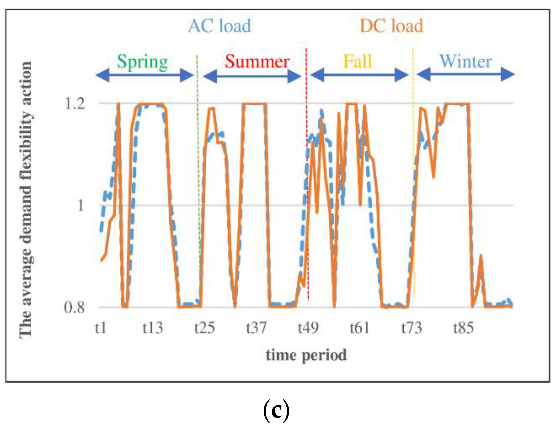
4.2.3. DFP Equations

The DFP equations of AC and DC distribution networks are presented in this section.

The equations of the DFP in the AC network are presented in (39)–(44): ($\forall i\in {\Omega }_{DF }^{ac}, \forall t\in {\mathsf{\Omega }}_T$).

$$P_{i,t}^{dac}=P_{i,t}^{daco}\ast {\gamma }_{i,t}^{ac}$$

(39)

$$Q_{i,t}^{dac}=Q_{i,t}^{daco}\ast {\gamma }_{i,t}^{ac}$$

(40)

$${\gamma }_{{}_{i,t}}^{ac}\le (1+{\gamma }_i^{\max }{\lambda }_i^{ac})$$

(41)

$${\gamma }_{i,t}^{ac}\le (1-{\gamma }_i^{\min }{\lambda }_i^{ac})$$

(42)

$${\displaystyle \sum _{t\in {\mathsf{\Omega }}_T}^{}{d}_t\ast P_{i,t}^{dac}}={\displaystyle \sum _{t\in {\mathsf{\Omega }}_T}^{}{d}_t\ast P_{i,t}^{daco}}$$

(43)

$${\displaystyle \sum _{t\in {\mathsf{\Omega }}_T}^{}{d}_t\ast P_{i,t}^{dac}}={\displaystyle \sum _{t\in {\mathsf{\Omega }}_T}^{}{d}_t\ast Q_{i,t}^{daco}}$$

(44)

$P_{i.t}^{daco}$ and $Q_{i.t}^{daco}$ in (39) and (40) show the amount of active and reactive demand of bus i in the AC distribution network without DFP and ${\gamma }_{i,t}^{ac}$ indicates the decision variable for demand pattern variation. The demand flexibilities are modeled by (41) and (42), where ${\gamma }_i^{max}$ and ${\gamma }_i^{min}$ identify the maximum potentials of growth and reduction for the demand in each hour. Moreover, ${\lambda }_i^{ac}$ is a binary variable, i.e., bus i does not contribute to the DFP if ${\lambda }_i^{ac}=0$. Although the load consumption pattern is variable, the energy consumption during the study period should remain constant, according to (43) and (44).

In addition, the DFP equations in the DC distribution network are presented in (45)–(48): ($\forall id\in {\Omega }_{DF }^{dc}, \forall t\in {\mathsf{\Omega }}_T$).

$$P_{id,t}^{ddc}=P_{id,t}^{ddco}\ast {\gamma }_{id,t}^{dc}$$

(45)

$${\gamma }_{id,t}^{dc}\le (1+{\gamma }_{id}^{\max }{\lambda }_{id}^{dc})$$

(46)

$${\gamma }_{id,t}^{dc}\le (1+{\gamma }_{id}^{\min }{\lambda }_{id}^{dc})$$

(47)

$${\displaystyle \sum _{t\in {\mathsf{\Omega }}_T}^{}{d}_t\ast P_{id,t}^{ddc}}={\displaystyle \sum _{t\in {\mathsf{\Omega }}_T}^{}{d}_t\ast P_{id,t}^{ddco}}$$

(48)

where, $P_{id.t}^{ddco}$ in (45) shows the amount of active demand of bus id in the DC distribution network without DFP and ${\gamma }_{id,t}^{dc}$ indicates the decision variable for the demand pattern variation. The demand flexibilities are modeled by (46) and (47), where ${\gamma }_{id}^{max}$ and ${\gamma }_{id}^{min}$ identify the maximum potentials of growth and reduction for the demand in each hour, which has the same value as the AC network. Moreover, ${\lambda }_{id}^{dc}$ is a binary parameter, i.e., if ${\lambda }_{id}^{dc}=0$ then the bus i does not contribute to the DFP. Equation (48) indicates that the total energy consumption of the DC distribution network should remain constant.

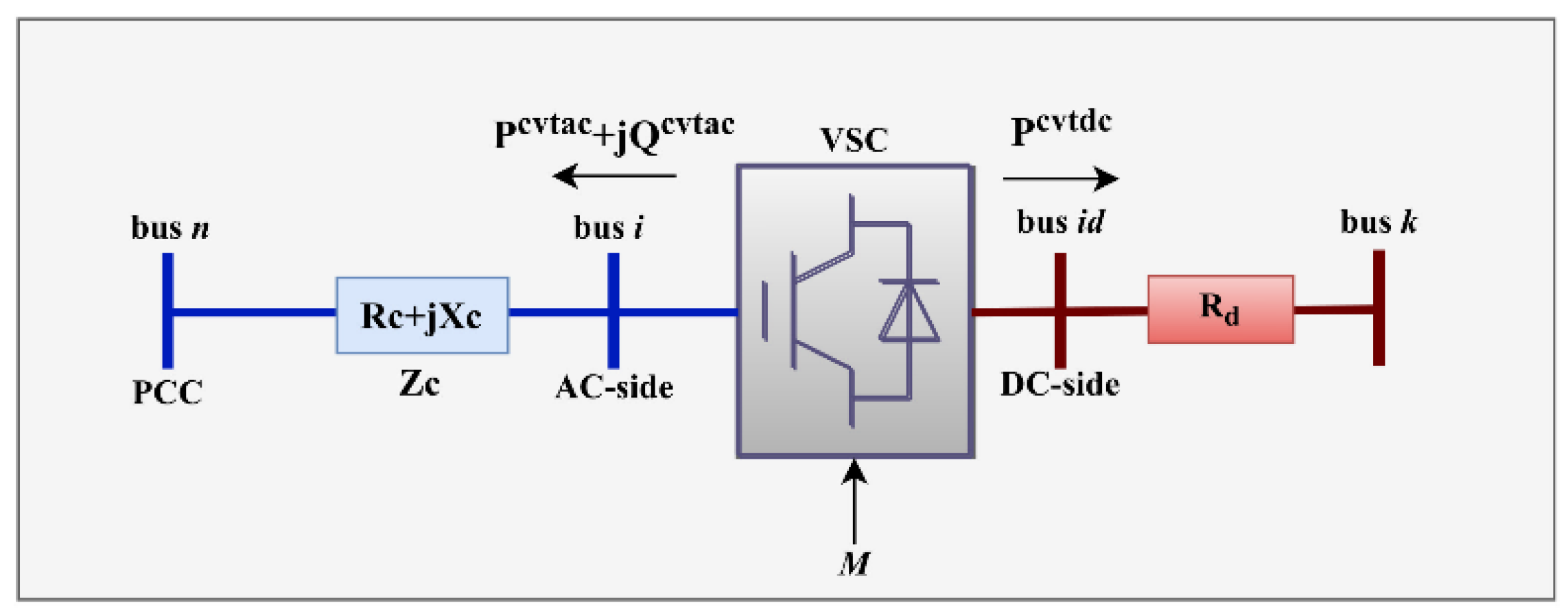
4.2.4. Modeling of VSC

In this paper, VSCs are installed to convert the AC-DC powers in the distribution network. The DC side of the VSC converters is a monopolar circuit and its model is depicted in Figure 2. The impedance $Z_c$ of the converter includes the connecting elements between the AC network (bus n) and the AC side of the converter (bus i). These elements include transformers, phase reactors, and/or low-pass filters. The relationship between AC base voltage and DC base voltage is in the form of (49) [37].

$$V_{base}^{ac}=K_{vsc}{V}_{base}^{dc}$$

(49)

The value of the constant in (49) ($K_{vsc}$) depends on the type of VSC and the Pulse Width Modulation (PWM) strategy. In this paper, $K_{vsc}$ is considered to be $\sqrt{3}/\left(2\sqrt{2}\right)$. Therefore, the base voltage level of AC and DC distribution networks are equal to 11 kV and 17.96 kV, respectively. The relationship between the AC and DC sides’ voltages of the converter is presented in (50), where M is the PWM’s amplitude modulation index.

$$V_{i.p.u}^{ac}=M_{i.id}{V}_{id.p.u}^{dc}$$

(50)

VSC constraints are presented in (51)–(54): ($\forall i\in {\Omega }_{cvt }^{ac}, \forall id\in {\Omega }_{cvt }^{dc}, \forall t\in {\mathsf{\Omega }}_T$,$\forall s\in {\mathsf{\Omega }}_S$).

$$P_{id,t,s}^{cvtdc}+P_{i,t,s}^{cvtac}+Plos{s}_{i,t,s}^{cvt}=0$$

(51)

$$Plos{s}_{i,t,s}^{cvt}=0.02\ast \left|P_{i,t,s}^{cvtac}\right|$$

(52)

$${(P_{i,t,s}^{cvtac})}^2+{(Q_{i,t,s}^{cvtac})}^2\le S_{i,\max }^2$$

(53)

$$Q_{i,t,s}^{cvtac}=P_{i,t,s}^{cvtac}\tan ({\Psi }_i)$$

(54)

The power connection between the AC and DC distribution networks is defined as (51). $Plos{s}_{i,t,s}^{cvt}$ expresses the VSC losses due to power exchange between AC/DC networks. According to [33], the losses can be considered to be 2% of the power supply to the AC distribution network, which is mentioned in (52). Normal VSC performance is limited by the maximum apparent power specified in (53). VSC reactive power can be controlled by a direct set point according to (53) or as a function of the converter power factor $\tan \left({\Psi }_i\right)$ according to (54). In this paper, in order to show the effect of reactive power control of VSCs on increasing the HC and reducing energy losses, first, the power factor is considered to be equal to 1, so that VSCs exchange only active power. Then, (54) is used to control the reactive power of VSCs and investigate its effect on the objective functions.

4.3. Linearization

The equations presented in the previous sections are linearized by the following hypotheses:

(1)

The typical power flow equations in AC and DC distribution networks that are illustrated in (9), (10), and (29), are nonlinear and non-convex. Reasonably, utilizing these power flow terms in the optimization problems is difficult. Therefore, they are linearized by taking into consideration two practical assumptions. The first one is regarding the bus voltage magnitudes, in an AC and DC distribution system, to be close to the nominal value $V_{nom}$ The second assumption is that the voltage angle difference ${\theta }_{ij}$ through the AC line is tiny, leading to the trigonometric estimates, i.e., $\sin ({\theta }_{ij})={\theta }_{ij}$ and $\cos ({\theta }_{ij})=1$ [37]. In addition, the voltage magnitude at bus i and id can be represented as the summation of the nominal voltage and a minor deviation $\mathsf{\Delta }{V}_{i/id}$, i.e., $V_{i/id}=V_{nom}+\mathsf{\Delta }{V}_{i/id}$.

(2)

The modulation index (M) of each VSC should be limited in order to prevent over-modulation and excessive harmonics. The upper limit of M can be selected as $M^{max}=1$ and the lower limit as $M^{min}=V_{ac,pu}^{min}/V_{dc,pu}^{max}$, which is usually the upper and lower voltage limits, i.e., 0.95 p.u and 1.05 p.u, respectively. By defining the variable $H=M^{-1}$, the upper and lower limits of H are considered equal to 1.1 and 1. Additionally, by defining ($H=1+dH+\mathsf{\Delta }H$) and dH equal to 0.05, the value of the new variable, i.e., $\mathsf{\Delta }H$, is limited to $\pm 0.05$. So, we have $M=H^{-1}$ [37].

(3)

The variables $\mathsf{\Delta }H$, $\mathsf{\Delta }V,$ and θ have small values and therefore their multiplication can be considered to be zero [37].

Therefore, according to the above hypotheses, (9), (10), and (29) become linear and convex as presented in (55) to (57): ($\forall id\in {\Omega }_{n }^{dc}, \forall i\in {\Omega }_{n }^{ac}, \forall t\in {\mathsf{\Omega }}_T$,$\forall s\in {\mathsf{\Omega }}_S$).

$$P_{ij,t,s}^{ac}=V_{nom}(\mathsf{\Delta }{V}_{i,t,s}^{ac}-\mathsf{\Delta }{V}_{j,t,s}^{ac})g_{ij}-V_{nom}^2{b}_{ij}{\theta }_{ij,t,s}$$

(55)

$$Q_{ij,t,s}^{ac}=-V_{nom}(\mathsf{\Delta }{V}_{i,t,s}^{ac}-\mathsf{\Delta }{V}_{j,t,s}^{ac})b_{ij}-V_{nom}^2{g}_{ij}{\theta }_{ij,t,s}$$

(56)

$$P_{id.jd,t,s}^{dc}=V_{nom}(\mathsf{\Delta }{V}_{id,t,s}^{dc}-\mathsf{\Delta }{V}_{jd,t,s}^{dc})G_{id,jd}^{dc}$$

(57)

Equations (55) and (56) present the AC lines’ active and reactive power flows and (57) shows the DC lines active power flow. However, the linearized relationship between AC-DC sides voltage of VSC that is described in Section 4.2.4 is presented in (58).

$$\mathsf{\Delta }{V}_{id,t,s}^{dc}=\mathsf{\Delta }{V}_{i,t,s}^{ac}(1+dH)+\mathsf{\Delta }{H}_{i.id,t,s}+dH-\mathsf{\Delta }{V}_{id,t,s}^{dc}$$

(58)

The active and reactive losses of the AC distribution network and active losses of the DC distribution network are presented in (59) to (61): ($\forall id \in {\mathsf{\Omega }}_n^{dc}$, $\forall i \in {\mathsf{\Omega }}_n^{ac}$, $\forall t \in {\mathsf{\Omega }}_T$, $\forall s \in {\mathsf{\Omega }}_S$).

$$P{L}_{ij ,t ,s}^{ac}=r_{ij}({(P_{ij ,t ,s}^{ac})}^2+{(Q_{ij ,t ,s}^{ac})}^2)/V_{nom}^2$$

(59)

$$Q{L}_{ij ,t ,s}^{ac}=x_{ij}({(P_{ij ,t ,s}^{ac})}^2+{(Q_{ij ,t ,s}^{ac})}^2)/V_{nom}^2$$

(60)

$$P{L}_{id.jd,t,s}^{dc}=r_{id,jd}^{dc}{(p_{id.jd,t,s}^{dc})}^2/V_{nom}^2$$

(61)

Equations (53), (59)–(61) contain quadratic variables, which can be linearized using the piecewise method. Also, (52) includes the absolute function that can be linearized by two piecewise functions:$Plos{s}_{i,t,s}^{cvt}=0.02\ast P_{i,t,s}^{cvtac} if P_{i,t,s}^{cvtac}\ge 0$ and $-Plos{s}_{i,t,s}^{cvt}=0.02\ast P_{i,t,s}^{cvtac} if P_{i,t,s}^{cvtac}\le 0$.

Finally, the transformed version of (7), (8), and (28) are presented in (62) to (64): ($\forall id\in {\Omega }_{n }^{dc}, \forall i\in {\Omega }_{n }^{ac}, \forall t\in {\mathsf{\Omega }}_T$,$\forall s\in {\mathsf{\Omega }}_S$).

$$P_{i,t,s}^{netac}={\displaystyle \sum _{\begin{array}{l}j\in {\mathsf{\Omega }}_n^{ac}\\ i\ne j\end{array}}(P_{ij,t,s}^{ac}+0.5P{L}_{ij,t,s}^{ac})}$$

(62)

$$Q_{i,t,s}^{netac}={\displaystyle \sum _{\begin{array}{l}j\in {\mathsf{\Omega }}_n^{ac}\\ i\ne j\end{array}}(Q_{ij,t,s}^{ac}+0.5Q{L}_{ij,t,s}^{ac})}$$

(63)

$$P_{id,t,s}^{netdc}={\displaystyle \sum _{\begin{array}{l}jd\in {\mathsf{\Omega }}_n^{dc}\\ id\ne jd\end{array}}(P_{id.jd,t,s}^{dc}+0.5P{L}_{id.jd,t,s}^{dc})}$$

(64)

4.4. Multi-Objective Optimization

Objective functions $F_1$ and $F_2$, discussed in Section 4.1, are two opposing objective functions and must be optimized simultaneously. In this paper, the ɛ-constraint method [6] is used to consider these contradictory objective functions. In this method, a function is considered as the main objective and the other one as an inequality constraint by considering the appropriate value of a particular parameter, called ε. Therefore, the multi-objective problem becomes single-objective and can be solved for different values of ε. In this paper, the function $F_1$ (HC) is selected as the main objective, and $F_2$ (energy losses) is considered as the inequality constraint. The model should be solved (calculating the $F_1$ value) for the different amounts of ɛ.

To choose the best compromise solution between the available solutions from the ε-constraint method, the fuzzy satisfying approach [6] is utilized in this paper. In this method, after calculating different objectives, fuzzy membership functions (${\overline{F}}_{1,2}$) are used. These functions (depicted in Figure 3) can be derived according to (65) and (66).

$${\overline{F}}_1=\{\begin{array}{l}0\begin{array}{cccc}& & & ,F_1\le F_1^{\min }\end{array}\\ \frac{F_1-F_1^{\min }}{F_1^{\max }-F_1^{\min }}\begin{array}{cc}& ,F_1^{\min }\le F_1\le F_1^{\max }\end{array}\\ 1\begin{array}{cccc}& & & ,F_1\ge F_1^{\max }\end{array}\end{array}$$

(65)

$${\overline{F}}_2=\{\begin{array}{l}1\begin{array}{cccc}& & & ,F_2\le F_2^{\min }\end{array}\\ \frac{F_2^{\max }-F_2}{F_2^{\max }-F_2^{\min }}\begin{array}{cc}& ,F_2^{\min }\le F_2\le F_2^{\max }\end{array}\\ 0\begin{array}{cccc}& & & ,F_2\ge F_2^{\max }\end{array}\end{array}$$

(66)

After normalizing different objectives, the best compromise solution candidate can be obtained using Distance Metric Method [38], as presented in (67).

$$Min{{\displaystyle \sum _{K=1,2}^{}\left|{\mu }_k-{\overline{F}}_k\right|}}^p$$

(67)

In (67), ${\mu }_K$ is the satisfaction level of the target functions from the policymaker’s point of view, which has values between (0–1). The final solution will be a compromise between the objective functions according to the membership amount of each function. It is noteworthy that K is the total number of objective functions and p is often equal to 2.

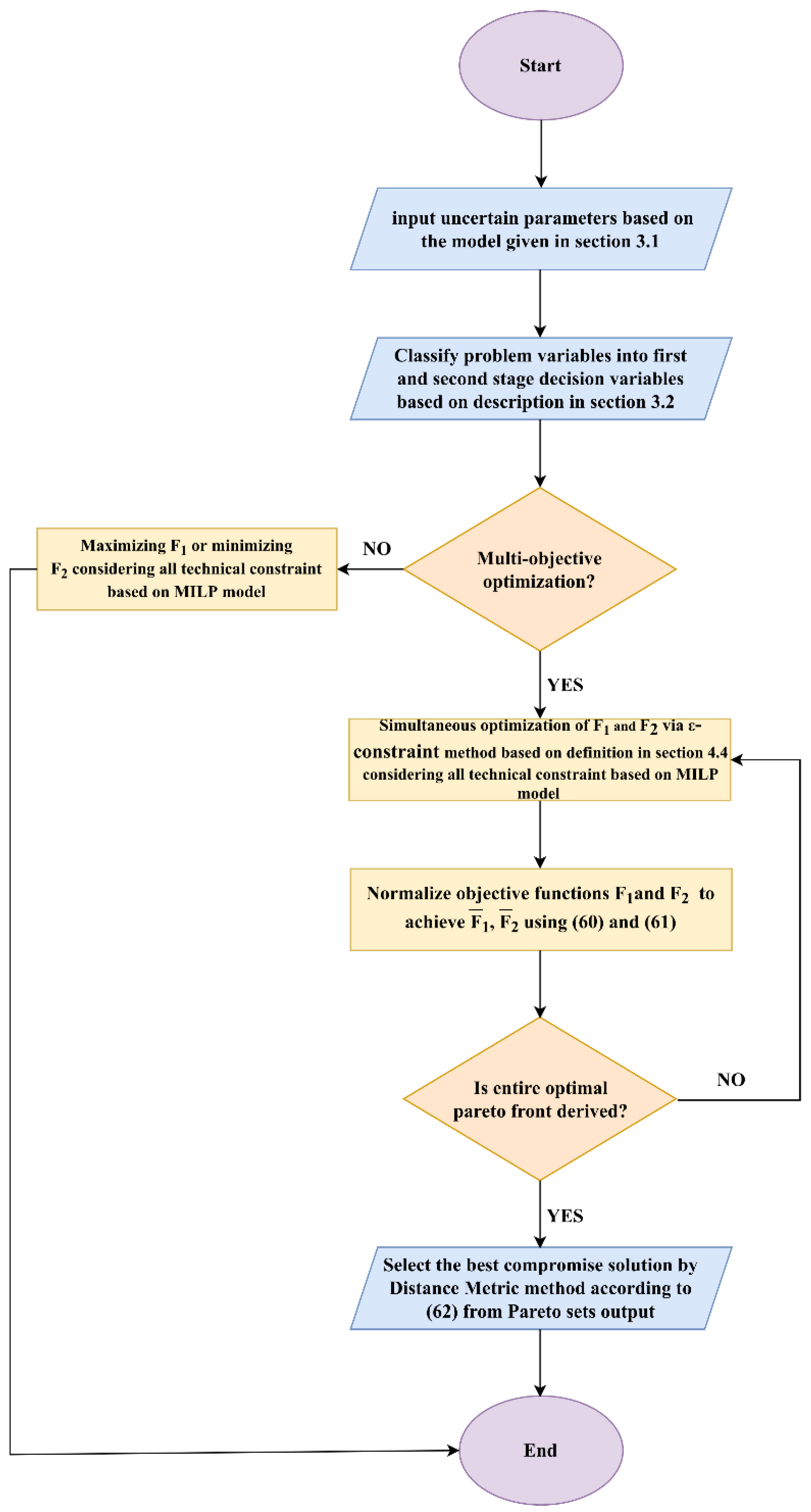
4.5. Solution Procedure

To clarify the proposed mathematical model, a summary of the solution procedure is presented in the flowchart depicted in Figure 4.

5. Simulation Results

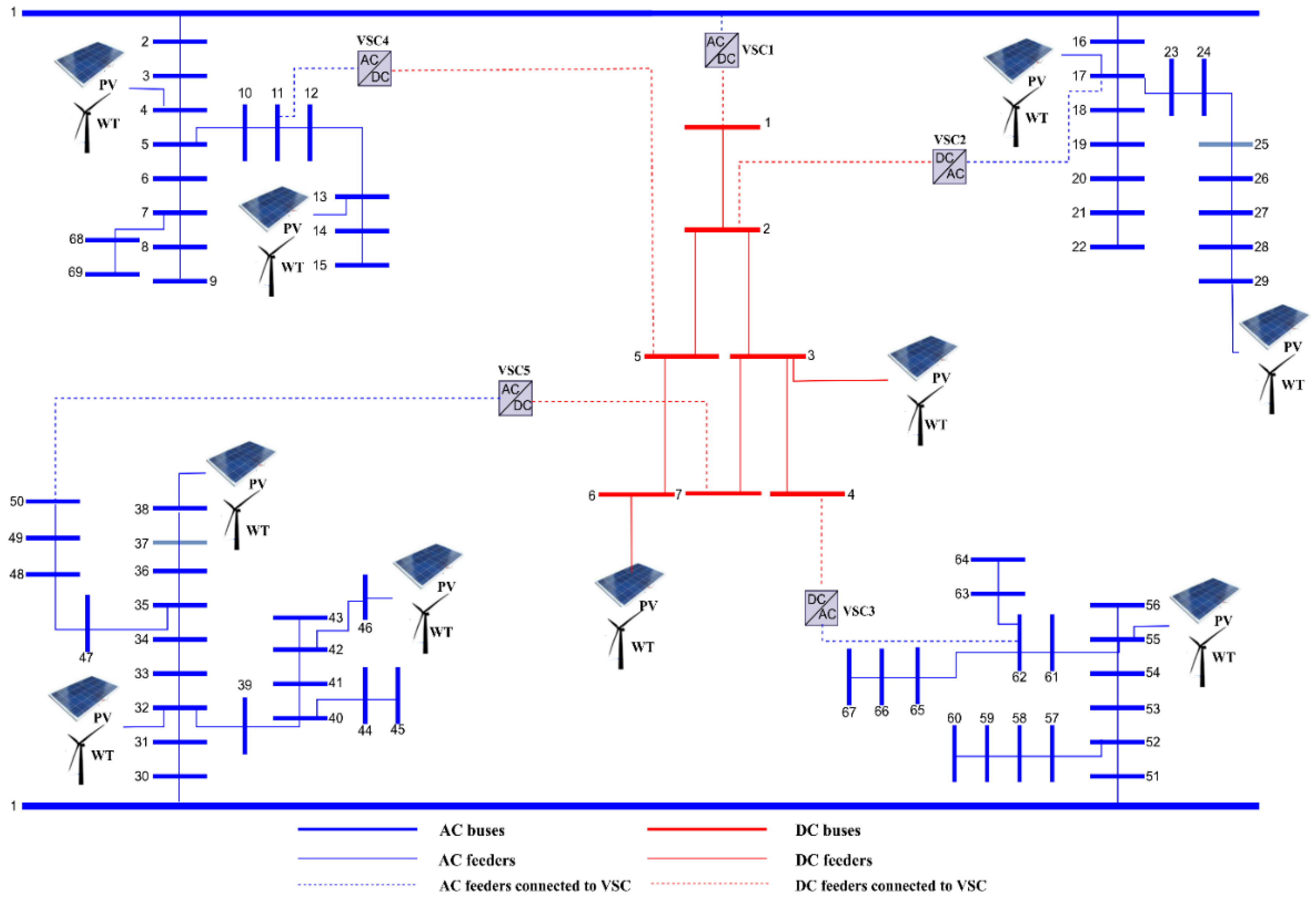
The proposed model is implemented in GAMS [39] environment and is solved using Gurobi solver, running on an Intel^® Core™ i7-4790k CPU @ 4.00GHz PC with 16 GB RAM.

5.1. Input Data

The proposed model is applied on a hybrid AC/DC distribution network consisting of 69 AC and 7 DC buses, as depicted in Figure 5. The total loads of AC and DC distribution networks are 4.56 MW and 5.1 MW, respectively. The base voltages of AC and DC distribution networks are 11 kV and 17.96 kV, respectively, and buses 1 of AC and DC distribution networks are considered as slack buses. The capacity of VSC1 is equal to 7 MVA, and the capacities of the rest of the VSCs are equal to 1 MVA. One year (8760 h) is considered as the planning horizon. To decrease the computation load, this 8760 h has been reduced to 96 h. In better words, one day of each season is selected as a sample, i.e., four days in total. WT/PV generation and AC/DC load data are given in [40]. Figure 6 shows the historical WT and PV generations and the AC and DC load consumptions. As described in Section 3.1, first, quite a few scenarios were generated for generation sources with the MCs, and then they are reduced to 4 scenarios with the fast-backward method. Candidate buses for installing WT and PV consist of buses 4, 13, 17, 29, 32, 38, 46, and 55 in the AC distribution network and buses 3 and 6 in the DC distribution network. The power factor limit of each WT and PV is considered to be 0.95 (lag/lead). The maximum percentage energy curtailment allowed for WT and PV is assumed to be 10%. Moreover, all buses in the AC and DC distribution networks could participate in the DFP (${\lambda }_i^{ac}=1$, $\forall i\in {\Omega }_{n }^{ac}$, ${\lambda }_{id}^{dc}=1$, $\forall id\in {\Omega }_{n }^{dc}$). Furthermore, the maximum demand flexibility of AC and DC distribution networks is assumed to be 20% for all buses.

5.2. Case Studies

To evaluate the effects of DFP and ANM on the HRES HC and energy losses, four different case studies are investigated as described in

Table 2. Specifications of case studies based on the types of RESs, objectives, and tools used in each case.

Case Study	Stochastic (Uncertainties)	RESs			Objectives		Tools
		WT Only	PV Only	Hybrid PV-WT	Max HC	Min Losses	DFP	ANM (QVSC)
1	✓	✓	✓	✓	✓	✘	✘	✓✘
2	✓	✓	✓	✓	✓	✘	✓	✓✘
3	✓	✓	✓	✓	✘	✓	✓✘	✓✘
4	✓	✘	✘	✓	✓	✓	✓	✓

✓/✘ denotes that the subject is/is not considered.

.

As can be seen, cases 1 and 2 are related to the HC enhancement, case 3 is focused on energy loss minimization, and case 4 considers the simultaneous (multi-objective) optimization of HC and energy losses. In the first three cases, the evaluation of the objective function is performed based on WT-only, PV-only, and hybrid PV-WT modes. Cases 1 and 2 are mainly focused on the DFP effect and the ANM influence, i.e., reactive power control of VSC (QVSC), is also investigated. Case 3 is focused on the losses minimization and the results are presented with/without DFP and QSVC. Case 4 investigates the multi-objective framework. So, only the results of hybrid mode (PV-WT) with the presence of DFP and QSVC are demonstrated and discussed.

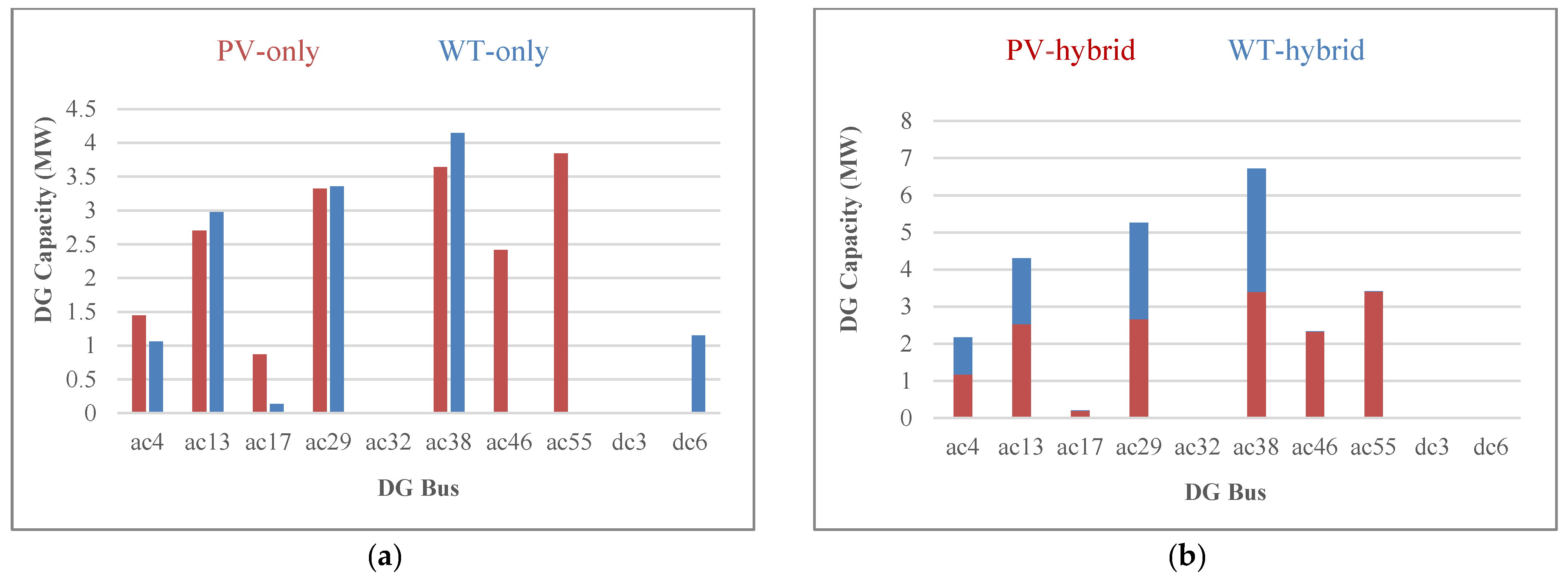
5.3. Case Study 1: Maximizing Hybrid PV-WT HC without DFP and with/without QVSC

In this case, the optimal capacity of WT and PV for maximizing the HC without DFP and with QVSC is derived during the study period. The results of this case are presented in

Table 3. HC, energy of sources, curtailment, losses, and energy exchange by VSC without DFP and with QVSC.

RESs	WT Capacity (MW)	PV Capacity (MW)	Total HC (MW)	Energy of Sources (GWh)	Energy Curtailment (GWh)	Energy Losses (GWh)	Energy Exchange by VSC (GWh)
WT-only	11.89	-	11.89	46.35	4.63	5.45	35.50
PV-only	-	15.63	15.63	27.48	2.74	4.52	29.15
Hybrid PV-WT	8.21	11.85	20.06	52.89	5.27	5.51	34.78

. As shown, the HC of PV-only mode is 31.5% higher than WT-only mode, still, the total energy generation of PV is equal to 59% of the energy generated by WT sources. The difference is due to the fact that WTs could track the demand variation better than PV in this network. So, WTs reach the network limits with less integrated capacity. The maximum energy curtailment is considered equal to 10% of the total energy generation by sources, which is at its maximum level as expected. When WT and PV generations are considered together, the amount of increase in energy generation of sources is 14% compared to WT-only mode and 93% compared to PV-only mode. The enhancement of HC in hybrid mode is 28% compared to PV-only mode in which the WT capacity has increased by 8.21 MW and the PV capacity has decreased only by 3.78 MW. Comparing the hybrid mode with the WT-only mode, the increase of HC is 37% in which the WTs capacity has decreased by 3.68 MW and the PVs capacity has increased by 11.85 MW. The amount of power exchanged between the two distribution networks by VSC in the PV-only mode is less than that in the other two modes due to less generation of PV than WT. Additionally, the large number of energy losses are due to zero generation of sources in the DC network as shown in Figure 7, which increases the energy losses by generating power in the AC network and transferring it to the DC network.

Figure 7 shows the optimal installed capacity of DGs in the candidate buses in three different modes without DFP and with QVSC. As can be seen, the installed capacity of DGs in the DC distribution network is zero in this case. In the hybrid mode, the installed capacity of DG in buses ac32 and ac46 is zero. In bus ac38, the WT capacity is 94% and in buses ac17 and ac55, the PV capacity is 100% of the total RESs installed capacity. In all of the other buses, the share of WT and PV capacity is almost equal. The difference between the share of WT and PV in various buses mainly depends on the specific spatial constraints, such as voltage and lines flow limits. As shown, the DG capacity of buses close to the upstream substation has a lower capacity than farther buses, mainly due to the voltage limitations. This is because of the fact that the farther buses from the upstream grid have a higher voltage drop and a larger amount of DG can be installed in these buses without causing any overvoltage issue.

Figure 8a shows the highest voltage of the network (at any location) vs. time period without DFP and with QVSC in scenario s₁. For the WT-only mode, high voltages level and voltage violations during the spring are more than in other seasons due to the high generation of WT. For PV-only, the high voltages level similarly tracks its source pattern, but the case is not as extreme as WT-only. In other words, despite the higher capacity of PV compared with the WT, the high voltages level in the PV-only mode is lower than in the WT-only mode and the voltage violations in the WT-only mode are more severe. This is due to the fact that WT sources generate noticeable power most of the time, leading to more effective utilization of the network capacity. However, the voltages level and violation of the hybrid PV-WT mode are more severe than the individual WT and PV modes, representing that the network HC is enhanced significantly.

Figure 8b shows the difference between the highest line loading in the network (at any line) and its maximum allowable power flow through the lines ($S_{ij}-S_{ij}^{max}$) vs. time period without DFP and with QVSC in scenario s₁. The high lines loading in PV-only mode follows its source pattern. The high lines loading and the line capacity violations in WT-only mode are more than in the PV-only mode. In addition, the case is more severe in the spring season. This is due to the same reason explained for the voltage levels. Besides this, the high lines loading and the lines capacity violation in hybrid PV-WT mode are more than individual WT and PV modes, which is due to the increased HC of the system.

Additionally, it is shown that how VSCs help to prevent the voltage drop and the high line loading with QVSC is to increase HC. For this purpose, active/reactive power of VSC connected between buses ac62 and dc4, power flow between bus ac1 to ac51, and reactive power of PV connected to bus ac55 of the hybrid mode are depicted in Figure 9 without DFP and with QVSC in the spring and for different scenarios (s).

In this area of the network, PV connected to bus ac55 has a 4.54 MW capacity producing active power and injecting/receiving reactive power. As shown in Figure 9a, most of the time, the active power of VSC is transferred from the AC network to the DC network due to 3 main reasons: (1) the power generation of sources in other buses, (2) the lack of installed capacity of sources in the DC network, and (3) the transferred power to this part of the network via the line between bus ac1 and ac51. As shown in Figure 9b,c, when active power is injected from the upstream grid to this part of the network, due to a lack of reactive power from the PV (depicted in Figure 9d) most of the time, the VSC tries to prevent voltage drop of the buses by injecting reactive power. In addition, when the PV starts generating active power (t₉–t₁₅) in this area, the active power flows in reverse to the upstream grid and VSC helps to control the voltage of the buses by absorbing the reactive power. This is one of the advantages of VSC, i.e., controlling the voltage of the distribution network by injecting/receiving reactive power leading to the HC enhancement.

The HCs, with and without QVSC in the hybrid mode without DFP are 20.06 MW and 19.6 MW and the energy losses are 5.51 GWh and 4.23 GWh. Therefore, VSCs can increase the HC and decrease the losses by injecting or absorbing reactive power into the AC distribution network. This is in addition to VSCs’ main role, i.e., the flexible transfer of active power between AC and DC lines.

5.4. Case 2: Maximizing Hybrid PV-WT HC with DFP and with/without QVSC

In this case, the optimal capacity of WT and PV for maximizing the HC with DFP and QVSC is derived, and the results are presented in

Table 4. HC, energy of sources, curtailment, losses, and energy exchange by VSC with DFP and with QVSC.

RESs	WT Capacity (MW)	PV Capacity (MW)	Total HC (MW)	Energy of Sources (GWh)	Energy Curtailment (GWh)	Energy Losses (GWh)	Energy Exchange by VSC (GWh)
WT-only	12.83	-	12.83	50.01	5.00	6.08	30.81
PV-only	-	18.25	18.25	32.08	3.20	4.79	32.64
Hybrid PV-WT	8.69	15.69	24.39	61.47	6.14	7.55	44.46

. Comparing the second case study with the first one, the HC is increased by 16.7% (2.62 MW) for PV-only mode, 7% (0.94 MW) for WT-only, and 21% (4.33 MW) for the hybrid PV-WT mode. It means that the DFP has a greater impact on the capacity of PV sources compared to the WT sources. This is because of the fact that PV generation is more concentrated on specific hours of the day causing more issues from the network perspective. Additionally, the energy losses in WT-only, PV-only, and hybrid PV-WT have increased with DFP. In other words, in this case (considering the DFP), the network is used more efficiently, and the flows of the lines are increased due to the enhanced HC, which has led to an increase in energy losses.

The installed capacities of WT and PV in various modes are demonstrated in Figure 10. Contrary to the first case study (without DFP), a part of WT installed capacity is located in the DC distribution network (for the WT-only mode). This is due to the application of DFP and providing the network relief for using the potentials of the DC network. However, in the hybrid and PV-only modes, the installed capacity of the sources in the DC distribution network is zero. Therefore, the power is generated in the AC network and should be transmitted to the DC network via VSC. This can increase the transmission capacity through VSC compared to the first case study.

Figure 11 shows the percentage of the hours that the voltages and lines loadings (any location in the network) have reached the allowed limits in different scenarios for different modes (PV-only, WT-only, and hybrid PV-WT) with/without DFP. Generally speaking, the voltage and line capacity violations of the WT-only mode are more than in the PV-only mode, which means that the WTs can utilize the network capacities more efficiently. Nevertheless, the hybrid PV-WT mode shows even a higher percentage of voltages and line loading limitations in comparison with the singular WT and PV modes. In addition, with the DFP, the occurrence of parameters reaching the allowed upper limits has increased. This means that the DFP can facilitate the efficient utilization of the network, similar to the hybrid RES’s consideration. Besides this, the voltage magnitude of the network has reached the allowed upper limits more frequently in comparison with the lines flows, which means that it is a more restricting parameter for the HC.

The scheduled DFP is a time and bus-dependent action. Therefore, the average DFP action for all buses in AC and DC distribution network is presented in Figure 12 for the PV-only, WT-only, and hybrid PV-WT modes. The average load actions in the PV-only and WT-only modes are more obvious during the hours that these sources generate their maximum output. Nevertheless, the average load action in the hybrid PV-WT mode is clearer when the PV has its maximum output. This means that the DFP has a more intense impact on the PV capacity installation, as mentioned earlier.

The HCs of PV-WT mode considering the DFP (case 2) with and without QVSC is 24.39 MW and 23.37 MW with the associated energy losses of 7.55 GWh and 5.78 GWh, respectively. A simple comparison with case 1 indicates that the HC is increased more when the QSVS is considered (comparing 0.46 MW and 1.02 MW enhancement of HC due to DFP). In other words, the DFP can facilitate the utilization of the network more efficiently when the QSVC is considered. Using the DFP and QSVC together leads to a network where almost all of the buses’ voltages and lines’ loadings reach their maximum allowable values. This means utilizing all of the potentials to increase the HC of the network.

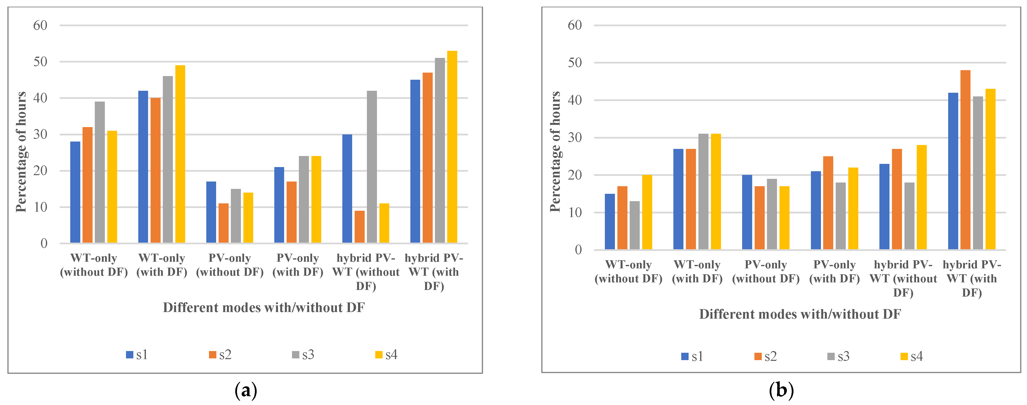
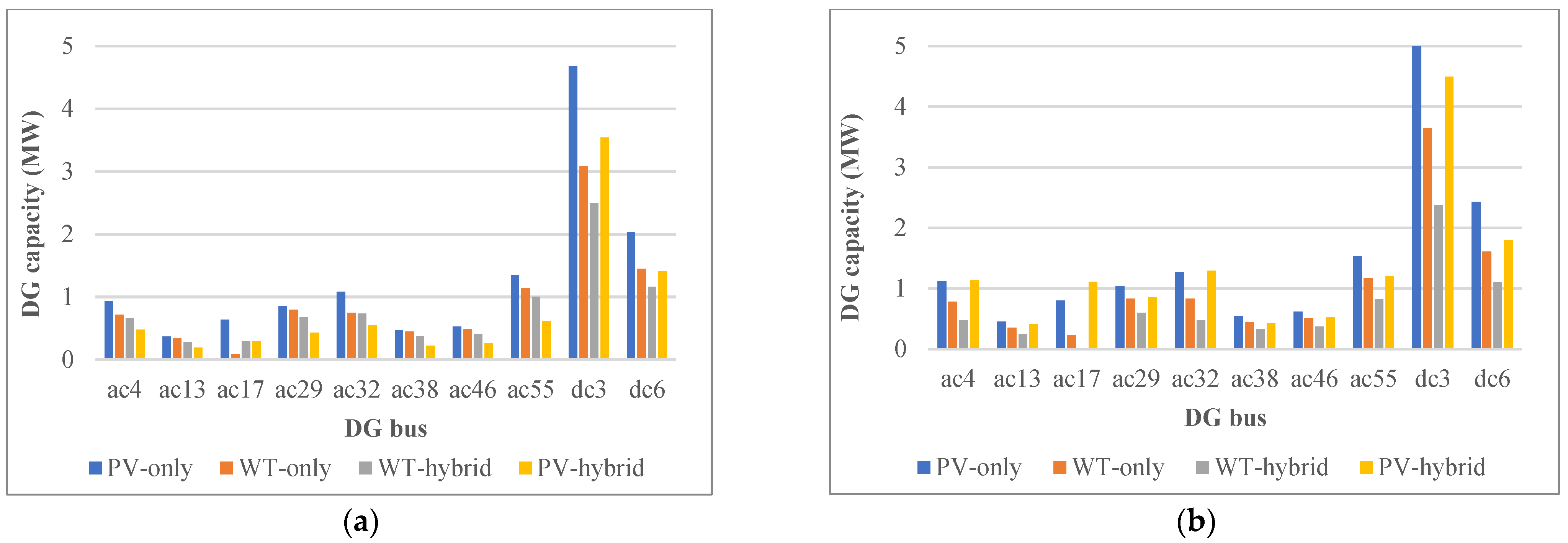
5.5. Case Study 3: Minimization of Losses for Hybrid PV-WT with/without DFP and QVSC

The discussed case in this section demonstrates the impact of HRES with DFP and QVSC on the energy loss reduction of the network. Therefore, it has been tried to determine the optimal capacity of single RESs (PV-only and WT-only) and HRES (hybrid PV-WT) in order to reduce the energy losses of the network. In this case, the HC is ignored as an objective function and both DFP and QVSC are used to only reduce the energy losses.

Table 5. Energy losses in three modes: PV-only, WT-only, and Hybrid PV-WT with/without DFP and with QVSC.

RESs	Without DFP		With DFP
	HC (MW)	Energy Losses (MWh)	HC (MW)	Energy Losses (MWh)
WT-only	9.35	649.23	10.43	574.10
PV-only	12.99	984.50	15.61	854.23
Hybrid PV-WT	16.16	475.97	20.05	405.00

shows the minimized energy losses and the associated HC in three modes: PV-only, WT-only, and hybrid PV-WT with/without DFP and with QVSC.

It is clear that the energy losses are a lot lower compared with cases 1 and 2, where the HC was the objective function. In addition, the losses of the PV-only mode are larger than the other two modes. Besides this, in the hybrid PV-WT mode, the energy losses are less than in the single RESs modes. This is because in the case of HRES, the higher generated power causes less injected power from the upstream grid and the local consumption of the power leads to less power flowing through the network. In addition, DFP shifts the load from the minimum generation and maximum demand periods to the maximum generation and minimum demand periods. This causes the power to be consumed more locally and reduces the reverse power flow, which consequently reduces the energy losses.

Figure 13 shows the installed capacity of sources in different locations for three modes: PV-only, WT-only, and hybrid PV-WT with/without DFP and with QVSC. As can be seen, compared to the HC enhancement strategy (cases 1 and 2), all sources have installed capacity in both AC and DC networks. In fact, due to low losses of the DC lines, the capacity of sources in the DC network is increased compared with the previous cases.

As shown, when the DFP is used, the energy losses and HC with QVSC are equal to 405 MWh and 20.05 MW, respectively. Without QVSC, these values are 501.8 MWh and 19.43 MW, respectively. With QVSC, the energy losses have decreased by 96.8 MWh and the HC has increased by 0.62 MW, which shows the beneficial effect of QVSC on increasing the HC and reducing the energy losses. In fact, due to local VSC reactive power support, the tension on the AC lines is reduced alleviating the energy losses.

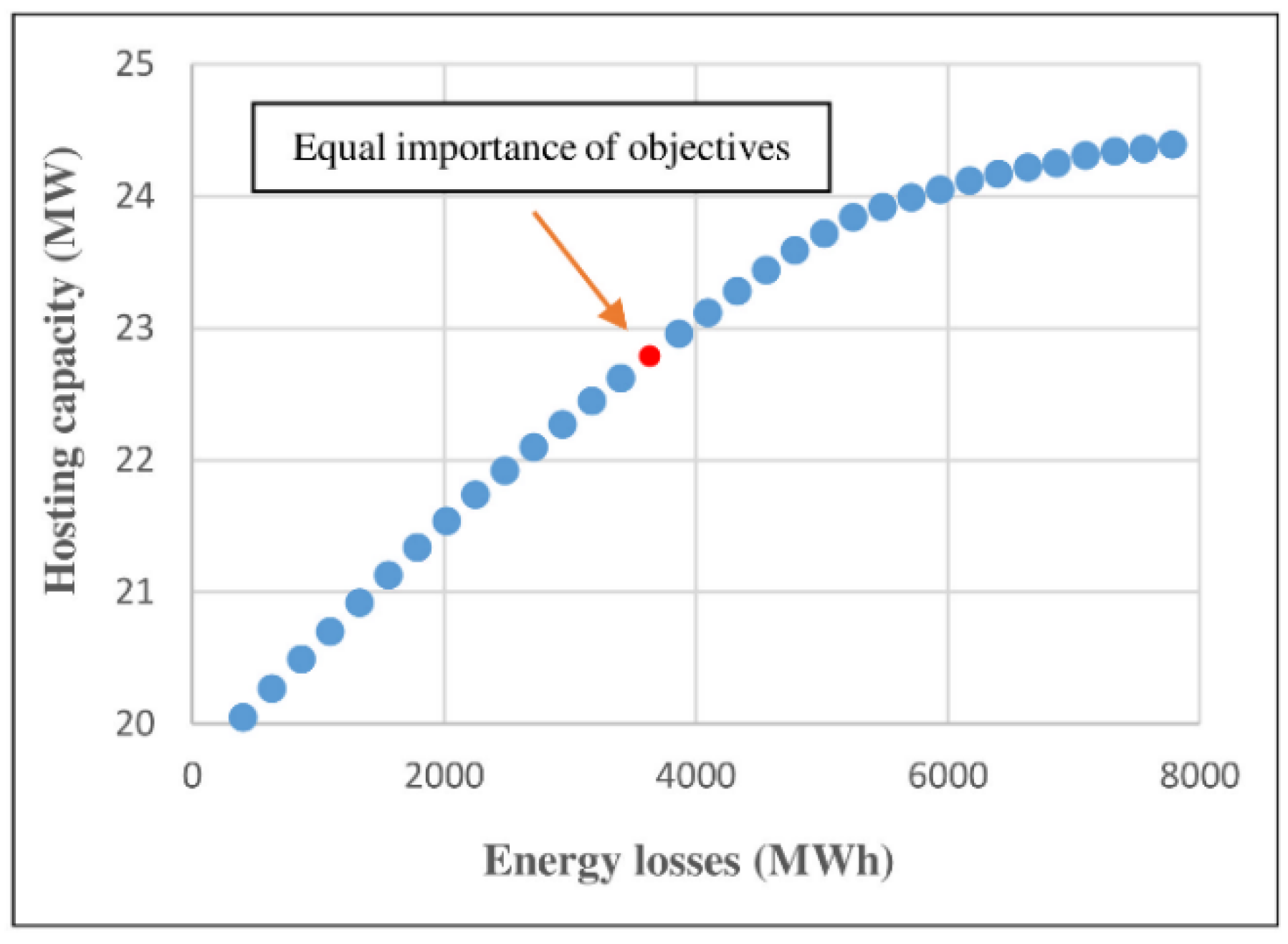
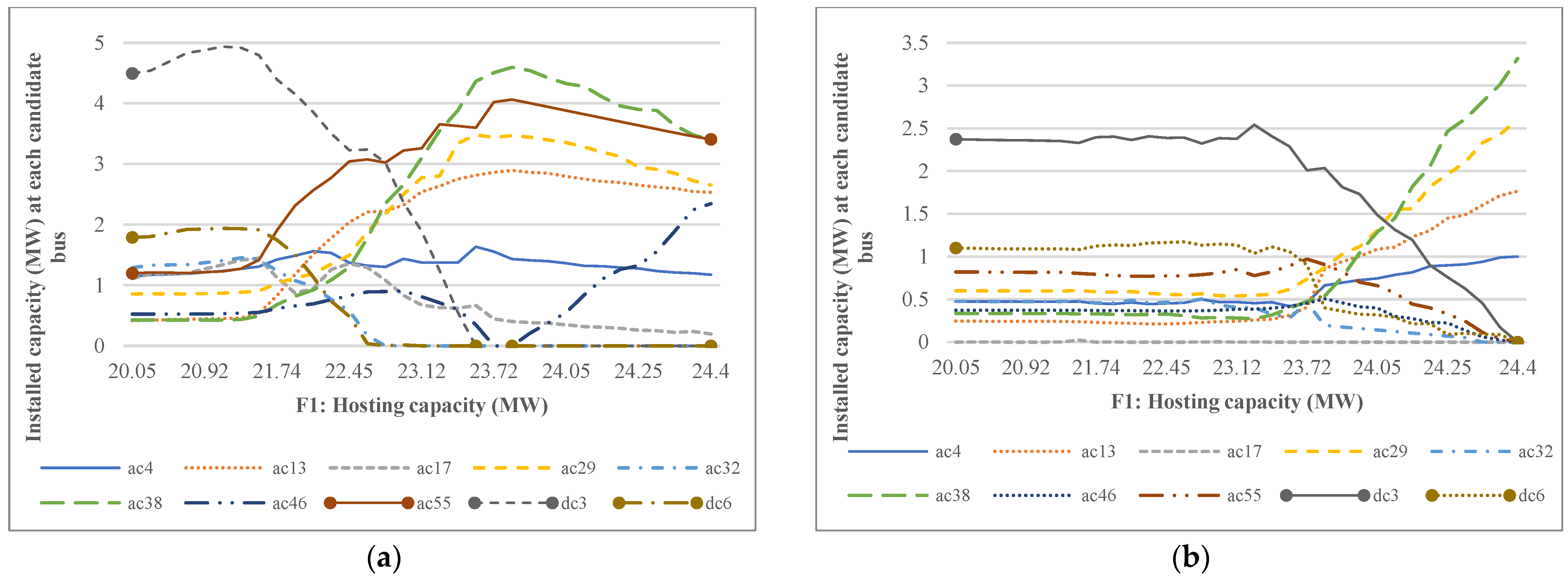
5.6. Case Study 4: Optimization of Hybrid PV-WT HC and Losses with the DFP and QVSC

Enhancing the HC increases the energy losses, which is contrary to the goals of DNO. Therefore, in this case study, an attempt has been made to trade off between these two objectives. As mentioned in case 2, the maximum HC is 24.39 MW with the associated energy losses of 7.55 GWh. Additionally, case 3 has demonstrated that the minimum energy loss is 405 MWh, and its associated HC is 20.05 MW.

As described in Section 4.4, this paper uses the ε-constraint method for calculating the Pareto front of two objectives, i.e., the minimum energy losses and the maximum HC. This method varies the values of ε for energy losses to optimally calculate the HC. In other words, the ε is increased from $F_2^{min}$ to $F_2^{max}$ smoothly and $F_1$ is maximized while the decision variables reach their optimal values. Setting the problem for minimization of the energy losses, $F_2^{min}$ can be calculated by solving the formulation with the objective function presented in (2). In addition, by solving the problem with the objective function presented in (1), the HC will be maximized and $F_2^{max}$ is the associated energy losses of this case. Figure 14 illustrates the Pareto optimal front considering energy losses and HC as the objective functions. It is obvious that the energy losses are increased when the HC is enhanced, showing the conflict between these objectives.

All of the points of the Pareto front are optimal from the DNO’s perspective. The decision-maker should choose the final optimal solution in accordance with the network requirements and the importance of each function for the policymakers. For example, if the HC is more important, its maximum value can be selected to be 24.39 MW with the energy losses being on its maximum value, i.e., 7.55 GWh. On the other hand, if the energy losses are more important, their value can be minimized up to 0.405 GWh with a minimum associated HC, i.e., 20.05 MW. In other words, the best HC is associated with the worst energy losses and vice versa, and the DNO must decide to stand between these two extreme cases according to the importance of objectives. Using the fuzzy satisfaction criterion and distance metric methods, described in Section 4.4, and selection of equal importance for the objectives (${\mu }_1=1 , {\mu }_2=1)$, the final trade-off solution is specified with the red point in Figure 14. At this point, the HC is 22.79 MW, and the energy losses are 3.63 GWh. If the HC is more important from the DNO’s point of view, they can choose a smaller threshold for the energy losses. For example, if ${\mu }_1=1 \mathrm{and} {\mu }_2=0.9$, the optimal HC and energy losses are equal to 23.12 MW and 4.09 GWh, respectively.

It is noteworthy that when the QVSC is considered without the DFP (case 1), the maximum HC is 20.06 MW with the energy losses being equal to 5.51 GWh. However, with the DFP, according to the presented Pareto front, when the HC value is 20.05 MW, the energy loss is approximately equal to 0.405 GWh. This shows the significant impact of the DFP on reducing the energy losses as well as increasing the HC. Additionally, when the DFP is considered without the QVSC (case 2), the maximum HC value was 23.37 MW with the energy loss being equal to 5.78 GWh. However, with the QVSC, according to the presented Pareto front, when the HC is equal to 23.37 MW, the energy loss is around 4.44 GWh. This shows the impact of the QVSC on reducing energy loss while enhancing the HC.

The variation in the importance of these objectives can change the installed capacity of WT and PV throughout the network. Figure 15 shows the changes in installed PV and WT capacities at the selected buses vs. the HC, considering both DFP and QVSC. At low values of HC, the WT and PV sources are installed on all of the candidate buses having more or less the same capacity. However, with the increase of HC, the installed capacity of PV and WT sources in some buses has been reduced (even to zero) and in some other buses, there is an increase in the RESs installed capacity. For example, the installed capacity of PV sources in dc3, dc6, and ac32 buses has been reduced to zero and the installed capacity of WT sources has decreased in dc3, dc6, ac32, ac46, and ac55 buses. In other words, with the increase of HC, the installed capacity of PV and WT sources has been focused on a few specific buses.

Generally speaking, the difference in the installed capacity of different buses can lead to an increase in the energy losses, due to the high values of active and reactive power flows of the network lines. Nevertheless, in the lower levels of HC, the RESs-based DGs supply the local consumers causing lower energy losses. As can be seen, with the increase of the HC from 23.28 MW onwards, the capacity of PV sources has been almost constant, and the capacity of WT sources has increased. Therefore, increasing in energy losses is mainly due to the increase in the installed capacity of WT sources.

5.7. Economic Analysis

Some basic economic analyses regarding the connection of RESs to the AC/DC networks are presented in this section. This paper investigates the effect of HRES along with DFP and QVSC on the HC enhancement in three modes: PV-only, WT-only, and hybrid PV-WT. Without DFP and in PV-only and hybrid PV-WT modes, the PV units are installed in the AC network. In addition, with DFP and in the WT-only mode, WT has a non-zero installed capacity in the DC network.

These cases, generally PV in the AC network and WT in the DC network, require more AC-DC and DC-AC converters. Therefore, connecting them to the associated networks comes at a cost.

Table 6. Total investment cost of converters and HC in three modes with/without DFP and with QVSC.

DFP	RESs	Additional Cost of Converters ($)	HC (MW)
Without DFP	WT-only	0	11.89
	PV-only	101,595	15.63
	PV and WT in AC and DC network (multi-location/ hybrid mode)	77,025	20.06
	PV in DC network and WT in AC network (single-location/ hybrid mode)	0	19.37
With DFP	WT-only	4830	12.83
	PV-only	118,625	18.25
	PV and WT in AC and DC network (multi-location/ hybrid mode)	101,985	24.39
	PV in DC network and WT in AC network (single-location/ hybrid mode)	0	21.81

shows the HC and the total investment cost of converters to connect RESs to the distribution network in various cases. The investment cost of AC-DC and DC-AC converters is considered to be 4200 $/MW and 6500 $/MW [41].

According to the table, the additional investment cost of converters in hybrid PV-WT mode is lower than in PV-only mode with and without DFP. It shows that when WT and PV are installed together in multi-locations (hybrid mode), they reduce the additional investment cost of converters in addition to enhancing the HC. Moreover, when WT and PV are installed in single-location (PV and WT in DC and AC networks, respectively), the total investment cost of converters becomes zero. Obviously, this comes at the cost of lowering the HC compared with the case of HRES in multi-locations. However, the HC is still larger than the HC of individual RESs modes. Therefore, it can be said that if it is chosen to place HRES in a single location of the proper network, the total investment cost of converters is reduced, and at the same time the HC increases compared to WT-only and PV-only modes. This shows the advantages of using hybrid AC/DC distribution networks and considering the HRES (hybrid PV-WT) at the same time.

5.8. Discussion

The proposed model in this paper is a multi-objective framework for increasing the HC and decreasing the energy losses. This model considers the hybrid RESs deployment mathematical model that can incorporate any kind of DGs considering their uncertainties using scenario-based stochastic programming. In this model, both DSM and ANM schemes have been considered simultaneously, which makes the proposed model more comprehensive. ANM schemes are DGs curtailment, DGs reactive power control, and VSCs reactive power control. Nevertheless, without loss of generality, other ANM schemes such as OLTC transformer, storage, and network reconfiguration are not considered, which can be straightforwardly added to the model.

In general, for HC studies, 8760 h of the year should be considered to demonstrate the accurate performance of the proposed model. However, due to the computation burden, one specific day of each season (totally, 96 h) is chosen to consider the frequent variability of RESs throughout the year. In addition, in order to be more realistic, the uncertainty of RESs output, which may occur at any specific time, is modeled via scenario-based stochastic programming.

The developed model was originally formulated as NonLinear Programming (NLP). Therefore, due to the noticeable size of the investigated test network, the nonlinearity and complexity of the accurate power flow equations, and the absolute expressions, the solution time was about 29 h. So, in order to reduce this computational burden, the proposed NLP model has been converted to a Mixed Integer Linear Programming (MILP) model. After providing a MILP model, the solution time has decreased considerably to 11 h, which shows the efficiency of the proposed model. It should be noted that the HC studies are conducted for planning purposes and consequently, this solution time can be considered acceptable. However, it is worth noting that the conversion process of the NLP to MILP is based on some hypothesis, which makes the proposed model non-accurate. However, the simulation studies have demonstrated that both MILP and NLP models have reached the same results.

6. Conclusions

This paper proposes a multi-objective, multi-source, and multi-period stochastic optimal linear power flow-based assessment framework to simultaneously optimize the hybrid PV-WT HC and energy losses via the ɛ-constraint method in a hybrid AC/DC distribution network considering all technical limitations and uncertainty of RESs. The main included technical limitations are the power flow equations of the AC and DC networks. The proposed model considers the common ANM schemes such as reactive power control and power curtailment of RESs. Additionally, the reactive power control of VSC is investigated as a new scheme of ANM in the HC studies. Moreover, one of the most significant DSM programs, i.e., DFP, is considered in the problem formulation. The simulation results show that one of the ways to reduce the effects of RESs variability is to use RESs in a complementary way, which makes them utilize the network’s capacity more efficiently, consequently increasing the HC and reducing the energy losses. Additionally, if DFP is used with HRES, the utilization of a network’s capacity becomes even more efficient, and the HC and energy losses become more optimized. In addition, one of the potentials of a hybrid AC/DC distribution network is the presence of VSC and its capabilities. It has been shown that in addition to the flexible transfer of active power between the two networks, it can increase the HC and reduce the energy losses by controlling its reactive power. The proposed method can lead to the optimal utilization of a hybrid AC/DC distribution network in order to increase HC and reduce the energy losses based on the proposed stochastic MILP model. The results elicited from the presented model can be used to offer incentives for DGOs. Therefore, each fraction of DNO revenues achieved by energy loss reduction is given to DGO in a way that decision of DGO would be compatible with the DNO requirements. These encouragements can also be taken into account in the connection costs. Such studies can be investigated in future works.

References

1. Bagherzadeh, L.; Shayeghi, H.; Pirouzi, S.; Shafie-khah, M.; Catalão, J.P. Coordinated flexible energy and self-healing management according to the multi-agent system-based restoration scheme in active distribution network. IET Renew. Power Gener. 2021, 15, 1765–1777. [Google Scholar] [CrossRef]
2. Chen, H.; Gao, L.; Zhang, Z. Multi-objective optimal scheduling of a microgrid with uncertainties of renewable power generation considering user satisfaction. Int. J. Electr. Power Energy Syst. 2021, 131, 107142. [Google Scholar] [CrossRef]
3. Hossain, M.; Jahid, A.; Islam, K.Z.; Alsharif, M.H.; Rahman, M. Multi-objective optimum design of hybrid renewable energy system for sustainable energy supply to a green cellular networks. Sustainability 2020, 12, 3536. [Google Scholar] [CrossRef]
4. Hussain, M.; Gao, Y. A review of demand response in an efficient smart grid environment. Electr. J. 2018, 31, 55–63. [Google Scholar] [CrossRef]
5. Venkatesan, C.; Kannadasan, R.; Alsharif, M.H.; Kim, M.-K.; Nebhen, J. A novel multiobjective hybrid technique for siting and sizing of distributed generation and capacitor banks in radial distribution systems. Sustainability 2021, 13, 3308. [Google Scholar] [CrossRef]
6. Rabiee, A.; Mohseni-Bonab, S.M. Maximizing hosting capacity of renewable energy sources in distribution networks: A multi-objective and scenario-based approach. Energy 2017, 120, 417–430. [Google Scholar] [CrossRef]
7. Bajaj, M.; Singh, A.K. Performance assessment of hybrid active filtering technique to enhance the hosting capacity of distorted grids for renewable energy systems. Int. J. Energy Res. 2022, 46, 2783–2809. [Google Scholar] [CrossRef]
8. Mulenga, E.; Bollen, M.H.; Etherden, N. A review of hosting capacity quantification methods for photovoltaics in low-voltage distribution grids. Int. J. Electr. Power Energy Syst. 2020, 115, 105445. [Google Scholar] [CrossRef]
9. Estorque, L.K.L.; Pedrasa, M.A.A. Utility-scale DG planning using location-specific hosting capacity analysis. In Proceedings of the 2016 IEEE Innovative Smart Grid Technologies-Asia (ISGT-Asia), Melbourne, VIC, Australia, 28 November–1 December 2016; pp. 984–989. [Google Scholar]
10. Capitanescu, F.; Ochoa, L.F.; Margossian, H.; Hatziargyriou, N.D. Assessing the potential of network reconfiguration to improve distributed generation hosting capacity in active distribution systems. IEEE Trans. Power Syst. 2014, 30, 346–356. [Google Scholar] [CrossRef]
11. Sun, W.; Harrison, G.P. Wind-solar complementarity and effective use of distribution network capacity. Appl. Energy 2019, 247, 89–101. [Google Scholar] [CrossRef] [Green Version]
12. Ali, A.; Mahmoud, K.; Lehtonen, M. Maximizing hosting capacity of uncertain photovoltaics by coordinated management of OLTC, VAr sources and stochastic EVs. Int. J. Electr. Power Energy Syst. 2021, 127, 106627. [Google Scholar] [CrossRef]
13. Xu, X.; Xu, Z.; Li, J.; Zhao, J.; Xue, L. Optimal Placement of Voltage Regulators for Photovoltaic Hosting Capacity Maximization. In Proceedings of the 2018 IEEE Innovative Smart Grid Technologies-Asia (ISGT Asia), Singapore, 22–25 May 2018; pp. 1278–1282. [Google Scholar]
14. Fachrizal, R.; Ramadhani, U.H.; Munkhammar, J.; Widén, J. Combined PV–EV hosting capacity assessment for a residential LV distribution grid with smart EV charging and PV curtailment. Sustain. Energy Grids Netw. 2021, 26, 100445. [Google Scholar] [CrossRef]
15. Kazemi-Robati, E.; Sepasian, M.S.; Hafezi, H.; Arasteh, H. PV-hosting-capacity enhancement and power-quality improvement through multiobjective reconfiguration of harmonic-polluted distribution systems. Int. J. Electr. Power Energy Syst. 2022, 140, 107972. [Google Scholar] [CrossRef]
16. Xiao, J.; Li, Y.; Qiao, X.; Tan, Y.; Cao, Y.; Jiang, L. Enhancing Hosting Capacity of Uncertain and Correlated Wind Power in Distribution Network with ANM Strategies. IEEE Access 2020, 8, 189115–189128. [Google Scholar] [CrossRef]
17. Rawa, M.; Abusorrah, A.; Al-Turki, Y.; Mekhilef, S.; Mostafa, M.H.; Ali, Z.M.; Aleem, S.H.A. Optimal allocation and economic analysis of battery energy storage systems: Self-consumption rate and hosting capacity enhancement for microgrids with high renewable penetration. Sustainability 2020, 12, 10144. [Google Scholar] [CrossRef]
18. Divshali, P.H.; Söder, L. Improving PV dynamic hosting capacity using adaptive controller for STATCOMs. IEEE Trans. Energy Convers. 2018, 34, 415–425. [Google Scholar] [CrossRef]
19. Hamidi, A.; Nazarpour, D.; Golshannavaz, S. Smart grid adds to renewable resources hosting capacity: Collaboration of plug-in hybrid electric vehicles in volt/VAr control process. Int. J. Energy Res. 2018, 42, 601–615. [Google Scholar] [CrossRef]
20. Ding, F.; Mather, B. On distributed PV hosting capacity estimation, sensitivity study, and improvement. IEEE Trans. Sustain. Energy 2016, 8, 1010–1020. [Google Scholar] [CrossRef]
21. Panda, A.; Aviso, K.B.; Mishra, U.; Nanda, I. Impact of optimal power generation scheduling for operating cleaner hybrid power systems with energy storage. Int. J. Energy Res. 2021, 45, 14493–14517. [Google Scholar] [CrossRef]
22. Monforti, F.; Huld, T.; Bódis, K.; Vitali, L.; D’isidoro, M.; Lacal-Arántegui, R. Assessing complementarity of wind and solar resources for energy production in Italy. A Monte Carlo approach. Renew. Energy 2014, 63, 576–586. [Google Scholar] [CrossRef]
23. Hoicka, C.E.; Rowlands, I.H. Solar and wind resource complementarity: Advancing options for renewable electricity integration in Ontario, Canada. Renew. Energy 2011, 36, 97–107. [Google Scholar] [CrossRef]
24. Ajeigbe, O.A.; Munda, J.L.; Hamam, Y. Towards maximising the integration of renewable energy hybrid distributed generations for small signal stability enhancement: A review. Int. J. Energy Res. 2020, 44, 2379–2425. [Google Scholar] [CrossRef]
25. Liu, D.; Wang, C.; Tang, F.; Zhou, Y. Probabilistic assessment of hybrid wind-PV hosting capacity in distribution systems. Sustainability 2020, 12, 2183. [Google Scholar] [CrossRef] [Green Version]
26. Soroudi, A.; Rabiee, A.; Keane, A. Distribution networks’ energy losses versus hosting capacity of wind power in the presence of demand flexibility. Renew. Energy 2017, 102, 316–325. [Google Scholar] [CrossRef] [Green Version]
27. Ikeda, S.; Ohmori, H. Evaluation for maximum hosting capacity of distributed generation considering active network management. Int. J. Electr. Electron. Eng. Telecommun. 2018, 7, 96–102. [Google Scholar] [CrossRef] [Green Version]
28. Alvarez-Herault, M.-C.; N’doye, N.; Gandioli, C.; Hadjsaid, N.; Tixador, P. Meshed distribution network vs. reinforcement to increase the distributed generation connection. Sustain. Energy Grids Netw. 2015, 1, 20–27. [Google Scholar] [CrossRef]
29. Zhang, L.; Chen, Y.; Shen, C.; Tang, W.; Liang, J. Releasing more capacity for EV integration by DC medium voltage distribution lines. IET Power Electron. 2017, 10, 2116–2123. [Google Scholar] [CrossRef]
30. Chaudhary, S.K.; Guerrero, J.M.; Teodorescu, R. Enhancing the capacity of the AC distribution system using DC interlinks—A step toward future DC grid. IEEE Trans. Smart Grid 2015, 6, 1722–1729. [Google Scholar] [CrossRef]
31. Kaipia, T.; Salonen, P.; Lassila, J.; Partanen, J. Application of low voltage DC-distribution system—A techno-economical study. In Proceedings of the 19th International Conference on Electricity Distribution CIRED, Vienna, Austria, 21–24 May 2007; pp. 21–24. [Google Scholar]
32. Ahmed, H.M.; Eltantawy, A.B.; Salama, M.M. A planning approach for the network configuration of AC-DC hybrid distribution systems. IEEE Trans. Smart Grid 2016, 9, 2203–2213. [Google Scholar] [CrossRef]
33. Delkhosh, H.; Moghaddam, M.P.; Ghaedi, M. Multi-Objective Sizing of Energy Storage Systems (ESSs) and Capacitors in a Distribution System. In Proceedings of the 2020 10th Smart Grid Conference (SGC), Kashan, Iran, 16–17 December 2020; pp. 1–6. [Google Scholar]
34. Soares, J.; Canizes, B.; Ghazvini, M.A.F.; Vale, Z.; Venayagamoorthy, G.K. Two-stage stochastic model using benders’ decomposition for large-scale energy resource management in smart grids. IEEE Trans. Ind. Appl. 2017, 53, 5905–5914. [Google Scholar] [CrossRef]
35. Conejo, A.J.; Carrión, M.; Morales, J.M. Decision Making under Uncertainty in Electricity Markets; Springer: New York, NY, USA, 2010. [Google Scholar]
36. Beerten, J.; Cole, S.; Belmans, R. Generalized steady-state VSC MTDC model for sequential AC/DC power flow algorithms. IEEE Trans. Power Syst. 2012, 27, 821–829. [Google Scholar] [CrossRef] [Green Version]
37. Ahmed, H.M.; Salama, M.M. Energy management of AC–DC hybrid distribution systems considering network reconfiguration. IEEE Trans. Power Syst. 2019, 34, 4583–4594. [Google Scholar] [CrossRef]
38. Maghouli, P.; Hosseini, S.H.; Buygi, M.O.; Shahidehpour, M. A multi-objective framework for transmission expansion planning in deregulated environments. IEEE Trans. Power Syst. 2009, 24, 1051–1061. [Google Scholar] [CrossRef]
39. Rosenthal, R. GAMS, A User’s Guide; GAMS Development Corporation: Washington, DC, USA, 2012. [Google Scholar]
40. Chen, Y.-L. An interactive fuzzy-norm satisfying method for multi-objective reactive power sources planning. IEEE Trans. Power Syst. 2000, 15, 1154–1160. [Google Scholar] [CrossRef]
41. Lotfi, H.; Khodaei, A. Hybrid AC/DC microgrid planning. Energy 2017, 118, 37–46. [Google Scholar] [CrossRef]
Figure 1. Structure and components of hybrid AC/DC distribution network.
Sustainability 14 07558 g001
Figure 2. Schematic of a VSC converter station.
Sustainability 14 07558 g002
Figure 3. Normalization of the objective functions; (a) maximization (HC), (b) minimization (energy losses).
Sustainability 14 07558 g003
Figure 4. Solution procedure flowchart.
Sustainability 14 07558 g004
Figure 5. Single line diagram of the hybrid AC/DC distribution network and the candidate WT and PV buses.
Sustainability 14 07558 g005
Figure 6. The historical, (a) WT and PV generations, (b) AC/DC load consumptions.
Sustainability 14 07558 g006
Figure 7. Capacity of RESs in different locations of the network without DFP and with QVSC; (a) WT-only and PV-only, (b) hybrid PV-WT.
Sustainability 14 07558 g007
Figure 8. (a) Highest voltage of the network (at any location), (b) Difference between high lines loading (any line in the network) and its maximum allowable power flow; vs. time period in scenario s1 without DFP and with QVSC.
Sustainability 14 07558 g008
Figure 9. (a) Active power of VSC connected between buss ac62 and dc4 (hybrid mode), (b) Reactive power of VSC connected between buses ac62 and dc4 (hybrid mode), (c) Active power flow from bus ac1 to bus ac51 (hybrid mode), (d) Reactive power of PV connected to bus ac55 (hybrid mode); without DFP and with QVSC.
Sustainability 14 07558 g009aSustainability 14 07558 g009b
Figure 10. Capacity of RESs in different locations of the network with DFP and QVSC; (a) WT-only and PV-only, (b) hybrid PV-WT.
Sustainability 14 07558 g010
Figure 11. Percentage of the hours that the parameters have reached the allowed limits in different scenarios with/without DFP and with QVC; (a) voltages issue, (b) lines loading issue.
Sustainability 14 07558 g011
Figure 12. The DFP action vs. time period; (a) PV-only, (b) WT-only, (c) hybrid PV-WT.
Sustainability 14 07558 g012aSustainability 14 07558 g012b
Figure 13. Capacity of WT-only, PV-only, and hybrid PV-WT in different locations; (a) without DFP and with QVSC, (b) with DFP and with QVSC.
Sustainability 14 07558 g013
Figure 14. The Pareto front of optimal solutions considering energy losses and HC as objectives.
Sustainability 14 07558 g014
Figure 15. The capacity of (a) PV and (b) WT at the selected buses vs. the HC considering DFP and QVSC.
Sustainability 14 07558 g015