Day-Ahead Spot Market Price Forecast Based on a Hybrid Extreme Learning Machine Technique: A Case Study in China

Abstract

With the deepening of China’s electricity spot market construction, spot market price prediction is the basis for making reasonable quotation strategies. This paper proposes a day-ahead spot market price forecast based on a hybrid extreme learning machine technology. Firstly, the trading center’s information is examined using the Spearman correlation coefficient to eliminate characteristics that have a weak link with the price of power. Secondly, a similar day-screening model with weighted grey correlation degree is constructed based on the grey correlation theory (GRA) to exclude superfluous samples. Thirdly, the regularized limit learning machine (RELM) is tuned using the Marine Predators Algorithm (MPA) to increase RELM parameter accuracy. Finally, the proposed forecasting model is applied to the Shanxi spot market, and other forecasting models and error computation methodologies are compared. The results demonstrate that the model suggested in this paper has a specific forecasting effect for power price forecasting technology.

1. Introduction

With the promulgation of the No. 9 Document of Electric Power Reform, China has entered a new round of electric power system reform, and the market has gradually realized diversification. One of the most important features of the current power system reform is to restore the commodity nature of power, transform the original integrated distribution market into a free market, and realize the marketization of power transactions. At the same time, the electricity transaction price equation was changed from the government to a market transaction formation. Therefore, for market players, a more accurate understanding of the electricity price formation mechanism and the ability to forecast future trends in electricity prices will become an important link for the adaptation to market-oriented electricity trading.

In a market economy, the market mechanism plays a certain role in regulating the sustainable development of power and can effectively regulate the supply–demand relationship in the electricity market. The price of electricity is the fundamental basis for production and consumption behavior. To achieve the sustainable development goals of energy-saving and environmental protection, it is necessary to have more accurate electricity price forecasting so as to provide a more scientific and effective decision-making basis for the market players. In recent years, in order to achieve China’s sustainable development, China has been building a new energy system focused on promoting the consumption of new energy. On the one hand, effective electricity price forecasting can save the economic cost of the operation of the new power system and optimize the operation efficiency of market operators; on the other hand, one of the characteristics of the new power system is that the new energy generation capacity will increase the instability of the power system. Effective electricity-price forecasting can send power system regulation signals to the market players, effectively regulate the power system balance, and establish the stability and sustainable development of the power system.

The price of electricity is an economic reflection of the market operation mode, which is formed by the interaction of various factors. Therefore, it is complex and comprehensive. Importantly, the volatility of the spot market increases the difficulty of price forecasting. At present, many experts at home and abroad research the characteristics of spot market price formation to analyze the spot market price forecast, arriving at a number of notable conclusions. Among them, the forecasting methods are mainly divided into three methods: time series models, machine learning, and the combination of time series and machine learning.

The time series model represents a time series composed of a series of discrete numbers observed at a series of times by one or a group of variables, and are mainly the following: moving average method, weighted moving average method, exponential smoothing method, and trend forecasting method. The use of the time series model currently takes three main forms: (a) The use of optimization algorithms to correct the core parameters of the time series model to ensure that the weights of the time series and the fluctuations of the series are within a reasonable range, such as Wang Ruiqing et al. in the use of particle swarm algorithm to correct the weights of GM (1,2) to achieve the purpose of improving the accuracy of short-term electricity price forecasting [1]; (b) The time series model is mainly composed of four components: seasonal component, trend component, cyclical component, and residuals. Due to the fine time granularity of spot electricity price forecasting, more experts choose to correct for residuals [2,3]; (c) Using the adaptability of different time series models, multiple time series are combined with each other, for example, using generalized autoregressive conditionally heteroscedastic (GARCH) to ARIMA to correct for heteroskedasticity [4,5].

Time series models perform forecasting with the prerequisite assumption that historical trends and future development change in the same pattern, so when large external changes occur, a certain bias can occur. To overcome this drawback, many experts focus on machine learning algorithms, which are trained on a large amount of data by machine learning to analyze the interaction between forecast data and other factors to predict future trends. Machine learning is an interdisciplinary specialty, covering probability theory knowledge, statistics knowledge, approximate theory knowledge, and complex algorithm knowledge. It uses a computer as a tool and is committed to real-time simulation of human learning. It divides the existing content into knowledge structures to effectively improve learning efficiency. Machine learning is applied to forecasting in a similar way to time series: (a) Using echo state network (ESN), convolutional neural network, limit learning machine, and other algorithms, combined with load, historical price, and supply and demand as inputs, it can build relevant prediction models [6,7,8]. For example, Hafeez et al. Proposed a restricted Boltzmann machine (RBM) -based predictor module [9]; (b) Combining optimization algorithms with different machine learning algorithms to improve the prediction accuracy of machine learning [10,11,12,13]; (c) The focus of the first two approaches is on improving machine learning forecasting capabilities. Additionally, many experts focus on the correlation analysis of factors, using methods such as principal component analysis and maximum information coefficient to analyze the correlation of the factors related to prior electricity price [14,15,16], Hafeez et al. Used modified cultural information (MMI) to extract historical data features, and used a GWDO optimization algorithm combined with factored conditional restricted Boltzmann machine (FCRBM) to construct day-ahead load forecasting [17]. In terms of the way machine learning is used, more optimization is currently done for the model itself [18,19]; therefore, in this paper, we add the screening of historical data to these three ways to improve the reliability of the original data and achieve the optimization of the machine learning model.

In addition, some experts also combine time series and machine learning algorithms to form combined time series–machine learning models, which are combined in two ways: (a) Using time series models to correct for the prediction errors of machine learning [20,21]; (b) Decomposing the original data curve to form high-frequency data and low-frequency data, with high-frequency data using machine learning models for prediction and low-frequency data prediction using machine learning [22,23,24]. These two combined models have the risk of increasing the prediction error because a certain amount of error is generated in the error correction process and in the data decomposition process, and this error leads to an increase in the final prediction error [25,26].

In combination with the use of the three models mentioned above, the current ideas for building electricity price-forecasting models include the following: One is to decompose and reconstruct the original price series, that is, to decompose the original price series by using many modal decomposition algorithms and wavelet models [27,28]. Then the improved forecasting model is used to forecast different price decomposition sequences. Finally, the forecasted values of several decomposition sequences are reconstructed to form the final electricity price-forecasted values [29]. This method can decompose the volatility to a certain extent, reduce the impact of price volatility on the learning ability of the prediction model, and retain the original curve characteristics. However, this approach often makes it difficult to take the relevant factors into account, and thus cannot fully reflect the real-time changes in the market. Because the relevant factors can not completely correspond to each decomposition curve, the predicted effect will be affected in the process of model training. This kind of model still belongs to time series extrapolation. Another model is to analyze the formation characteristics of electricity price, taking electricity price and its related factors as the input of the model to improve the accuracy of the prediction model. This kind of model can reflect the real-time change of electricity price on the market and the relationship between different factors, and can reflect the structural change of the market to some extent [30]. But this type of model is strict regarding the choice of characteristic value, as the weak correlation with characteristic value will affect the forecast effect in the model training process, causing the deviation to increase [31,32,33].

According to the above analysis, some key elements are missing from the current studies on electricity price forecasting, namely:

(a)

Many current studies ignore the useless information brought by the large amount of electricity price data when screening data features, which not only causes a reduction in forecasting accuracy but also affects the operational efficiency of forecasting models [34].

(b)

The existing prediction models are generally based on a single sample set composed of features, which leads to the extraction of too much data, resulting in poor prediction accuracy [35,36].

In order to overcome the above shortcomings, this paper proposes a price forecasting model for day-ahead spot market based on hybrid extreme learning machine technology. Firstly, the formation mechanism of electricity price in the spot market is analyzed, the relevant factors of electricity price prediction in the spot market are sorted out, and the correlation degree of relevant factors of electricity price is verified by Spearman model. Secondly, the Criteria Importance Though Intercriteria Correlation (CRITIC) model is improved, the difference coefficient and Spearman model are used to improve the traditional CRITIC, the comprehensive weights of relevant factors are obtained, and the weights are assigned to the gray correlation (GRA) screen to obtain similar daily data, which can ensure that the prediction model will not cause overfitting due to data differences. Third, the Marine Predators Algorithm (MPA) is used to optimize the regularization coefficient and hidden layer node parameters of the traditional Regularized extreme learning machine (RELM) to obtain the best prediction model, and predict the predicted daily electricity price according to the best prediction model. Fourth, in order to further verify the prediction effect of the price prediction model based on the hybrid extreme learning machine technology proposed in this paper, MPA-RELM, GA-ELM, GA-SVM, ELM, and SVM are used as the reference for the prediction results. Additionally, according to the root mean square error (RMSE), the mean absolute error (MAE), the mean square error (MSE), and the residual sum of squares (SSE) act as a variety of prediction model output effect evaluation indicators. Through the case analysis of the actual data of the spot pilot in China, it is shown that the model proposed in this paper improves the accuracy of the original data to a certain extent, improves the generalization ability of the RELM model, and achieves greater accuracy of prediction results. This research has certain guiding significance for forecasting spot market price. The abbreviations and acronyms are in Abbreviations section.

The main contributions of this paper are as follows:

(1)

Through the analysis of sample factor correlation degree and sample factor similarity, a massive amount of data is cleaned up, the amount of data is reduced, the useful information is fully used, the accuracy of the RELM model is improved, and the calculation efficiency of the model is improved.

(2)

Considering the characteristics of the RELM model, the MPA model is used for optimization to reduce the probability of the prediction model falling into the local optimal solution.

(3)

A framework of electricity price forecasting based on similar days is proposed, which realizes 96-point forecasting in a day instead of single-point forecasting

According to the idea of constructing the forecast model, the following chapters of this paper are arranged as follows: the second chapter constructs the similar day screening model, mainly from the aspects of the formation mechanism of electricity price, relevant elements of electricity price and the construction of similar day screening model. The third chapter will build the RELM electricity price forecasting model based on MPA optimization. This part mainly introduces the RELM model and MPA model, combines the characteristics of the two models, and describes the forecasting process of the forecasting model. In the fourth chapter, a case study of the spot market in Shanxi Province of China will be carried out to verify the effectiveness of the model proposed in this paper. The last chapter will summarize the whole paper.

2. Extraction of Similar Days

2.1. Analysis on the Formation Mechanism of Electricity Price in Spot Market

The electricity price in the spot market is the result of many market factors. Since the construction of the spot market in China is in the initial stage, the rules of spot market operation in each pilot province are unique, which leads to differences in the operation conditions of the spot market and the laws of electricity price in each province [37]. Therefore, according to the similarities and differences between the construction of the European electricity market and the Chinese electricity market, this paper, combined with the general law of construction of spot markets in each province of China, proposes the steps of electricity price formation in Chinese spot market.

Both the Chinese spot market and the European spot market clearing price follow the principle of supply-demand balance, in which the supply side declares supply power according to the monotonic non-decreasing principle and the demand side declares demand power according to the monotonic non-increasing principle. The market equilibrium is the point where the two curves intersect and the price is the same for supply and demand schedules. This point determines the market clearing price and the corresponding quantity. Accepted offers and bids fall at the left of the intersection of the two curves and all of them are exchanged at the clearing price [38]. In addition, both the Chinese spot market and the European spot market set a threshold for the maximum price of the spot market. Markets have set thresholds for the maximum price of 1500 and 3000 Euros, respectively.

However, there are still many differences between the Chinese and European electricity markets. First, the Chinese day-ahead spot market is declared from 9:00 a.m. to 9:30 a.m., and the day-ahead clearing results are released at 5:30 p.m. on the same day, while the European day-ahead spot is from 8:00 p.m. to 12:00 p.m. Second, the European price clearing model mainly considers the capacity constraint of the contact line in the price area, but the Chinese spot market is a centralized and decentralized coexistence. Third, China’s electricity market is a dual-track market where the plan and market coexist, and the degree of marketization is lower than that of the European electricity market, so the plan will interfere with the price formation process, and the price will be abnormally spiked. Fourth, both the European and Chinese power markets have a large number of new energy transactions, but the Chinese power market has a policy of prioritizing the consumption of new energy, and the new energy is only reported but not quoted, resulting in the Chinese spot market price forming zero price with the new energy output. Fifth, the Chinese spot market is cleared every 15 min, forming 96 prices a day, but the European clearing interval is 1 h, with a total of 24 prices a day.

This paper summarizes the formation of the electricity price in the spot market as follows [39,40,41,42,43]:

(1)

The power grid dispatching center provides the trading center with the basic information of the power system according to the operation status of the power system, and the trading center releases the market public information to the market subjects according to the trading sequence;

(2)

According to market public information, the market subject discriminates the market supply-demand ratio, thermal power output, and New energy output, and formulates the trading strategy according to the market information;

(3)

According to the corresponding transaction clearing rules, the trading center will centrally match the transaction strategies of the sender and user sides to form a pre-clearing price;

(4)

The trading center sends the pre-clearing results to the power grid dispatching center for security verification. The power grid checks the clearing results according to the power system carrying capacity. If the verification is passed, the trading center forms a formal clearing price. If the verification is not passed, the trading center needs to re-match the transaction;

(5)

The trading center will send the final market price to the trading subject.

From the formation process of electricity price (Figure 1), it can be seen that the trend of electricity price is mainly affected by market public information, the output of different power generation entities, demand loads, market entities’ trading strategies and power system security. In the conventional electricity market, the supply and demand ratio of the market is one of the important bases for market entities to formulate strategies. At the same time, market entities will also formulate the latest trading strategies based on past experience. Therefore, in the incomplete information market, the impact of market entity strategies on electricity price-mapping can be done from market public information.

2.2. Identification of Electricity Price Forecasting Factors in Spot Market

According to the description in the previous section, the formation of spot market electricity price is formed by the joint action of a variety of factors. This paper summarizes the research on existing electricity price forecasting factors as follows: historical electricity price, market demand, thermal power output, New energy output, provincial load adjustment and market player strategy [44,45,46].

The history of electricity price tracks the electricity market before the result is divided into the day-ahead spot price and real-time spot prices. Market demand includes the market main body, the different time scales of market demand, market demand prediction deviation in the province and the provincial requirements, etc., Thermal power output includes the history and actual output of thermal power, scheduling, and modulation of and participation in peak shaving, etc. [47,48]. New energy output includes the historical output of New energy, forecast deviation of New energy output, and proportion of New energy output in market demand, etc. Provincial load adjustment mainly includes medium and long-term transaction power and inter-provincial spot transaction power [49,50]. The specific factors related to electricity price forecast as follows:

Table 1. Electricity price forecast related factors.

Species	Factors
History of electricity	Day-ahead spot price, real-time spot price;
Demand load in the province	Forecasting deviation of market demand load and market load;
Thermal power output	Historical actual output of thermal power, thermal power pre-dispatch output, thermal power participation in peak adjustment output;
New energy output	Historical output of new energy, forecast deviation of new energy output, proportion of new energy in market demand;
Inter-provincial demand load	Provincial adjustment of medium and long term trading electricity, inter-provincial spot trading electricity;

.

According to the research status at home and abroad, and combined with the actual market information release of spot pilot in China, this paper adopts Unified scheduling load, Inter-provincial demand load, New energy output and thermal power output as the core indicators of screening similar days of spot price forecast. In order to further confirm the correlation of relevant factors selected in this paper, the current spot electricity price of Shanxi province on 27 November 2021 is taken as an example (as shown in Figure 1 and Figure 2), and introduces Spearman correlation for correlation analysis. Spearman correlation coefficient can also be expressed as rank value. That is, Spearman correlation between two variables can be expressed as Pearson correlation between the rank values of two variables. Its main calculation formula is as follows:

$$r_s=1-\frac{6{\displaystyle \sum d_i^2}}{n(n^2-1)}$$

(1)

where d_i represents the rank difference between subjects, n represents the number of observations, and $r_s$ represents the correlation between two subjects.

Through the above Equation, we can get the correlations of Unified scheduling load, Inter-provincial demand load, New energy output and Thermal power output: 0.8214, 0.5790, −0.7954, and 0.9655, respectively. It can be seen that thermal power space has the strongest correlation to spot price, followed by the Unified scheduling load, and finally Inter-provincial demand load. In the selection of similar days, the correlation coefficient is taken as the relevant factor of weight.

2.3. Selection of Similar Days Based on Weighted Gray Relational Grade

2.3.1. Improvements to CRITIC

Criteria Importance Though Intercrieria Correlation (CRITIC) is an objective weighting method, and its weight composition mainly comes from the contrast intensity and the conflict of indexes. The comparative strength of the indicators indicates a value gap between options under the same indicator, which is calculated as standard deviation [51]. Indicator conflict indicates the correlation between qualitative changes. The correlation between indicators can be either positive or negative [52]. Traditional CRITIC uses standard deviation as its conflict criterion, but each index used in this paper has great difference and negative correlation, so single standard deviation can not reflect the difference [53]. Therefore, based on the basic principle of CRITIC, this paper uses the coefficient of variation to replace the standard deviation to express the index contrast strength [54,55].

$$C_v(j)=\frac{\delta (j)}{\mu (j)}$$

(2)

where $C_v(i)$ represents the difference coefficient of the index’s ith electricity price-related factor, $\delta (i)$ represents the standard deviation of the index’s ith electricity price-related factor, and $\mu (i)$ represents the average of the index’s ith electricity price-related factor. The information quantity of the factors related to the electricity price may be expressed as follows:

$$C_j=C_v(j){\displaystyle \sum _i^n(1-r_{ij})}$$

(3)

where $C_j$ represents the amount of information contained in the factor j and $r_{ij}$ represents the correlation between the factor i and the factor j. The weight $w_j$ of the relevant factors of the j electricity price may be expressed as follows:

$$w_j=C_j/{\displaystyle \sum _{j=1}^m{C}_j}$$

(4)

2.3.2. Weighted Gray Correlation

According to the above, the main factors related to the sifting of similar days are provincial load, transmission load, new energy power, and thermal power output. Therefore, build ${\xi }_t=[u_t^1,u_t^2,u_t^2,u_t^2]$ to represent the factors associated with day t. $u_t^1$ represents the amount of electricity in a province. $u_t^2$ represents outgoing load, $u_t^3$ represents new energy capacity, and $u_t^4$ represents thermal power capacity. First, all the factors related to electricity price are normalized and non-dimensional. According to the above correlation between new energy and electricity price has a negative correlation, so the minimization of new energy is adopted. The grey correlation coefficient for the ith factor of electricity price on day t and the ith factor on the forecast date shall be calculated as [56]:

$${\chi }_{tk}(n_i)=\frac{\underset{tk}{\min }\underset{n_i}{\min }{\Delta }_{tk}(n_i)+\mu \underset{tk}{\max }\underset{n_i}{\max }{\Delta }_{tk}(n_i)}{{\Delta }_{tk}(n_i)+\mu \underset{tk}{\max }\underset{n_i}{\max }{\Delta }_{tk}(n_i)}$$

(5)

In Equation (5), ${\Delta }_{tk}(n_i)=|x_0^{\text{'}k}(n_i)-x_t^{\text{'}k}(n_i)|$ represents the difference between the value of the n_i element on the forecast day and the value of the n_i element on the t day. $\underset{tk}{\min }\underset{n_i}{\min }{\Delta }_{tk}(n_i)$ represents the minimum difference value for all elements, and $\underset{tk}{\max }\underset{n_i}{\max }{\Delta }_{tk}(n_i)$ represents the maximum difference value for all elements. $\mu$ represents the resolution coefficient, which is 0.5. The correlation coefficients between different factors in different historical days can be calculated by the above Equation. The weighted gray relational degrees of different historical days and forecast days can be expressed as follows:

$${\varphi }_t={\displaystyle \sum _{t=1}^n{w}_t(\frac{1}{m}{\displaystyle \sum _{n_i=1}^m{\chi }_{tk}(n_i)})}$$

(6)

In Equation (6), $w_t$ is the weight obtained by the Equations (1)–(4), and n is the total number of factors related to the electricity price.

This paper constructs a similar day-screening model for electricity price forecasting according to CRITIC-GRA, mainly to screen historical day information similar to the forecast day, which can reduce the interference of relevant historical data on the forecast model and also solve the problem of bias generated by the screening data set. The specific process of the model is as follows:

(a)

Select the relevant factors of electricity price forecast, and use Spearman correlation to analyze the correlation of relevant factors;

(b)

Determine the forecast date, use the improved CRITIC model to calculate the relevant factors of the forecast date and the historical date, and obtain the comprehensive weight between the relevant factors;

(c)

Bring the weight of relevant factors obtained by CRITIC into the GRA model to obtain the correlation coefficient between different factors on different historical days;

(d)

The correlation coefficients of different historical days are sorted from large to small. The market information similarity between the previous historical day and the forecast day is the highest, and the electricity price similarity is the highest. On the contrary, the electricity price similarity is also lower.

(e)

The number of similar days can be selected according to the size of the similarity interval of the whole historical day, and the previous similar days are preferred. If the market is relatively stable and the similarity concentration is high, it can also be further determined according to the number of training arrays of the prediction model.

The CRITIC-GRA similar day-screening model constructed in this paper can bring the influencing factors of electricity price into the electricity price forecasting model on the basis of ensuring the authenticity of the original data. At the same time, the correlation between factors is added to the screening of similar days in the form of weight, so as to avoid the drawback that the factors affect the electricity price in equal proportion.

3. Construction of Electricity Price Forecasting Model

3.1. Regularized Extreme Learning Machine (RELM)

China’s electricity spot market construction is still in the initial stage, and there are many uncertainties regarding the price of electricity on the spot market. The spot price is characterized by strong volatility and nonlinearity, which increases the difficulty of electricity price forecasting. Therefore, the price-forecasting model of spot market needs to solve the nonlinear relation of electricity price to some extent. Regularized limit learning machine is an improvement to the traditional limit learning machine. The regularization coefficient is added to ELM, which can increase the generalization ability of ELM to some extent [57]. In this paper, RELM is used to construct the spatial mapping relationship between electricity price and related factors, which can improve the accuracy of electricity price prediction and enhance the anti-interference of the model. The RELM network can be represented as:

$$\min F=\underset{\delta }{\min }\left\{\frac{\lambda }{2}\right|\left|\xi \right|{|}^2+\frac{1}{2}\left|\right|\beta \left|{|}^2\right\}$$

(7)

where $\xi ={\displaystyle \sum _{}^{}{\beta }_{j}g(w_j·X_j+b_j)-t_j}$ is the sum of training errors, where $\left|\right|\xi |{|}^2$ and $\left|\right|\beta |{|}^2$ are empirical and structural risks, respectively, and $\lambda$ is the regularization coefficient. The weights matrix can be obtained by processing the Lagrange Equation (8):

$$\stackrel{⌢}{\beta }={(H^{T}H+\frac{I}{\lambda })}^{-1}{H}^{T}Z$$

(8)

where I is the identity matrix, Z is the parameter matrix of the model training settlement input, and H is the output matrix of the hidden layer.

In the prediction process, according to the results of previous training, the weight matrix w and the hidden layer offset matrix b are generated randomly. Then the hidden layer output weight matrix $\stackrel{⌢}{\beta }$ is calculated according to the ELM output function, forming the RELM regression model as Equation (9):

$$f={\displaystyle \sum _{i=1}^L{\stackrel{⌢}{\beta }}_{i}g(w_{i}x+b)}$$

(9)

3.2. Marine Predator Algorithm (MPA)

Marine Predators Algorithm (MPA) is a new meta- heuristic optimization algorithm proposed by Afshin Faramarzi and others in 2020. MPA optimization is divided into three stages: the initialization stage, the optimization stage, and the FADs effect or eddy current stage. The specific MPA optimization process can be described as follows [58]:

(1)

Initialization phase. Set algorithm parameters to initialize the location of the prey within the search scope. It can be described as:

$$X_0=X_{\min }+rand(X_{\max }-X_{\min })$$

(10)

In Equation (10), $X_{\max }$, $X_{\min }$ denote the search space of the prey, and rand(·) is a random number within (0, 1).

(2)

Optimization stage. The optimization phase is divided into early iteration, middle iteration and late iteration. At the beginning of the iteration, the current iterations are less than 1/3 of the maximum iterations. Predators are faster than prey, performing globes and updating prey through Brown random.

$$\begin{gathered} \{\begin{array}{c}stepsic{e}_i=R_B\otimes (Elit{e}_i-R_B\otimes pre{y}_i)\\ pre{y}_i=pre{y}_i+P•R_B\otimes stepsic{e}_i\end{array} \\ Iter<\frac{1}{3}\max \_Iter \end{gathered}$$

(11)

In Equation (11), $stepsice$ is the step size, $R_B$ is the Brownian walk random vector with normal distribution, $pre{y}_i$ is the prey matrix with the same dimension as the static matrix, $Elit{e}_i$ is the elitist matrix constructed by the top predator, $\otimes$ is a multiplicative operation item by item, P equals 0.5, and R is a (0, 1) uniform random vector. N is the population size, and $Iter$ and $\max \_Iter$ represent the current and maximum iterations.

In the middle of an iteration, the current iteration is less than 2/3 of the maximum. The population is divided into two parts, in which the prey does the levy movement, being responsible for the algorithm development in the search space. Predators do Brownian motion, being responsible for the algorithm’s exploration in the search space, shifting gradually from an exploration to a development strategy.

At the end of the iteration, the current iteration number is more than 2/3 of the maximum iteration number, mainly to improve the local development, the predator is slower than the prey speed, predator roaming based on levy.

$$\begin{gathered} \{\begin{array}{c}stepsic{e}_i=R_L\otimes (R_L\otimes Elit{e}_i-pre{y}_i)\\ pre{y}_i=Elit{e}_i+P•CF\otimes stepsic{e}_i\end{array} \\ Iter>\frac{2}{3}\max \_Iter \end{gathered}$$

(12)

In Equation (12), $R_L$ is the Levy distributed random vector, and $CF={(1-Iter/\max \_Iter)}^{(2·Iter/\max \_Iter)}$ is the adaptive parameter controlling predator movement compensation.

(3)

FADs effect or eddy current. Fish aggregation devices (FADs) or vortex effects often change the behavior of marine predators, which enables the MPA to overcome the premature convergence problem and adjust the local extremum.

$$pre{y}_i=\{\begin{array}{c}pre{y}_i+CF[X_{\min }+R_L\otimes (X_{\max }-X_{\min })]\otimes U\\ pre{y}_i+[FADs(1-r)+r](pre{y}_{r1}-pre{y}_{r2})\end{array}\begin{array}{l}r\le FADs\\ r>FADs\end{array}$$

(13)

In Equation (13), $FADs$ is the influence probability, takes 0.2, $U$ is the binary vector, r is the random number in (0, 1), r1, r2 is the random index of the prey matrix respectively.

3.3. MPA-RELM Model Construction

Through the explanation of RELM above, we know that the prediction precision of RELM is greatly influenced by the regularization coefficient $\lambda$ and the number of hidden layer nodes L. Therefore, the RELM model is further optimized by MPA to obtain more accurate regularization coefficient $\lambda$ and hidden layer node number L. The root mean square error (RMSE) of the training sample is selected as the fitness function of the MPA:

$$fitnes{s}_{RMSE}={(\frac{1}{n}{\displaystyle \sum _{t=1}^n({\stackrel{⌢}{x}}_t-x_t)})}^{1/2}$$

(14)

In Equation (14), ${\stackrel{⌢}{x}}_t$ represents the training prediction, $x_t$ represents the training observation, and n represents the number of training samples.

The specific process of MPA-RELM-based spot price forecasting algorithm is as follows:

(1)

Divide the similar day data selected by CRITIC-GRA above into training and testing sets and normalize them;

(2)

Set parameters such as the maximum number of iterations and population size. According to the Equations (1)–(10), the prey initialization position is set and the current iteration number is 0 to calculate the management matrix.

(3)

According to the three stages of the optimization process, continuously update the location of prey, complete the elite update, calculate the fitness value, and update the final position.

(4)

In combination with the FADs effect, the Equations (1)–(13) are used to update the prey so that the algorithm can iteratively jump out of the local optimal solution.

(5)

Evaluate and update the elite matrix and determine the relationship between the number of iterative operations and the maximum number of iterations. If the iterative algorithm is equal to the maximum number of iterations, the best iterative elitist matrix is output. Elitist matrix is the best key parameter of RELM, which is brought into RELM model for prediction. The specific process structure is shown in Figure 3.

3.4. Construction of a Day-Ahead Spot Market Price Prediction Model Based on Hybrid Extreme Learning Machine Technology

In this section, the improved electricity price forecasting hybrid algorithm, denoted as CRITIC-GRA-MPA-RELM, is developed and shown in Figure 4. Its main procedure is summarized as follows:

(1)

Data preprocessing

Aiming at the research on the formation mechanism of electricity price in the electricity market, combined with domestic and foreign research on spot electricity price forecasting models, collect and organize relevant data on electricity price forecasting.

(2)

Identify the core factors of electricity price forecasting

Based on the formation factors of electricity price in the spot market, combined with the actual operation information of spot pilots in various provinces in China, the relevant factors of electricity price prediction are screened out, and the Spearman correlation coefficient is used to calculate the influence degree of each factor on electricity price.

(3)

Build a similar day screening model

Similar day screening model consists of two parts: improved CRITIC and weighted grey relational degree. First, the factor correlation obtained by the Spearman correlation coefficient is replaced by the conflict index of the traditional CRITIC. Second, the difference coefficient is replaced by the standard deviation to calculate the contrast strength index of CRITIC. Third, the comprehensive weight of CRITIC is formed, and the gray relational degree model is given weight. Fourth, the original dataset is screened according to the improved CRITIC-GRA model to form a similar daily dataset.

(4)

Select the optimal model to predict

First, the data of similar days are divided into training set and test set. Second, using the training set data as the input of the model, the Marine Predator Algorithm (MPA) is used to optimize the RELM to obtain the optimal regularization coefficient and hidden layer nodes. Third, use the test set data as the optimal RELM model for prediction, and finally get the prediction result.

(5)

Model prediction result verification

In order to verify the validity of the model, according to the characteristics of the RELM model selected in this paper, MPA-RELM, GA-ELM, GA-SVM, ELM, and SVM are selected as the model prediction results reference, and SSE, MSE, RMSE, and MAE as model evaluation metrics.

$$SSE={\displaystyle \sum _{i=1}^m{(y_i-{\widehat{y}}_i)}^2}$$

(15)

$$MSE=\frac{1}{m}{\displaystyle \sum _{i=1}^m{(y_i-{\widehat{y}}_i)}^2}$$

(16)

$$RMSE=\sqrt{\frac{1}{m}{\displaystyle \sum _{i=1}^m{(y_i-{\widehat{y}}_i)}^2}}$$

(17)

$$MAE=\frac{1}{m}{\displaystyle \sum _{i=1}^m|y_i-{\widehat{y}}_i|}$$

(18)

where $y_i$ denotes the real electricity price and ${\widehat{y}}_i$ denotes the forecast electricity price.

(6)

Diebold–Mariano test

In order to better verify that the model proposed in this paper is superior to other models, the Diebold–Mariano test is used to determine whether there are significant differences between different prediction models. The DM test is a widely-used prediction test method [59,60,61,62].

Let $e_i^1$ and $e_i^2$ be the residuals for the two forecasts, i.e.,

$$e_i^1={\widehat{y}}_i^1-y_i,e_i^2={\widehat{y}}_i^2-y_i$$

(19)

and let $d_i$ be defined as one of the following

$$d_i={(e_i^1)}^2-{(e_i^2)}^2$$

(20)

Find the mean and standard deviation of a series d

$$d_{mean}=\frac{1}{m}{\displaystyle \sum _i^m{d}_i}$$

(21)

$${\gamma }_k=\frac{1}{m}{\displaystyle \sum _{i=k+1}^m(d_i-d_{mean})}(d_{i-k}-d_{mean})$$

(22)

where γ_k is the autovariance at lag k.

For h ≥ 1, define the Diebold–Mariano statistic as follows:

$$DM=\frac{d_{mean}}{\sqrt{[{\gamma }_0+2{\displaystyle \sum _{k=1}^{h-1}{\gamma }_k}]/n}}\sim N \left(0,1\right)$$

(23)

4. Case Analysis

Although foreign spot markets are more mature and have abundant data, there are relatively few studies on electricity prices in the Chinese spot market, and since the Chinese spot market is in its infancy, market players have a more urgent and practical need for electricity price forecasting in the Chinese spot market. Therefore, this paper mainly selects the 96 points-per-day data of the spot market in Shanxi Province from 1 October 2021 to 25 February 2022, and in order to better demonstrate the operation of the Shanxi spot market, this paper intercepts one week of data for display (Figure 5 and Figure 6).

Select MATLAB2019b as the simulation computing platform, the computer operating system is Windows 11, the memory is 16G, and the hard disk is 1T.

4.1. Similar Day Filter

The model instance dataset is mainly composed of the day-ahead spot electricity price data from 1 October 2021 to 25 February 2022, with a time granularity of 96 points-per-day. Among them, the data from 1 October 2021 to 24 February 2022 is used as the training set, and 25 February 2022 is used as the prediction day. The relevant factors on 25 February 2022 are shown in Figure 7. According to the similar daily screening model based on the improved CRITIC-GRA constructed above, the 147 sets of training set data were further extracted to obtain a more accurate training set, and the first 50 sets of training data sets were screened out according to the data requirements of RELM. The result is as follows:

In the process of screening similar days in this paper, the following conclusions can be drawn: First, thermal power output has the greatest impact on electricity price, so the similarity in this paper is affected by the similarity of thermal power output to a certain extent. Secondly, according to the similarity of various factors every day, it can be seen that the inter-provincial dispatch load on most days has a high similarity, indicating that the demand in the Shanxi spot market is basically stable, but the New energy has great uncertainty and is negatively correlated with spot electricity prices, which is in line with Shanxi province’s rule of preferential consumption of New energy. The sorting results of similar days are shown in Figure 8.

In this paper, the similarity of historical days is calculated, and the similarity interval of historical days is (0.627006, 0.878184). In this paper, the first 50 groups of similar days are selected for the following reasons: firstly, the historical days ahead of similar days are more related to the predicted daily electricity price. Secondly, the more obvious the similarity difference, the more stable the market operation, the stronger the correlation of factors, and the smaller the interference to the prediction model. Thirdly, 50 groups of historical data can prevent too much or too little data from affecting the training efficiency.

According to

Table 2. Similarity and ranking of similar days.

Time	Similarity	Ranking	Time	Similarity	Ranking
24 February 2022	0.878184	1	29 November 2021	0.773253	26
11 December 2021	0.846866	2	14 January 2022	0.770666	27
23 February 2022	0.839821	3	7 February 2022	0.766438	28
1 October 2021	0.835788	4	28 December 2021	0.766079	29
13 February 2022	0.824152	5	16 November 2021	0.765566	30
19 January 2022	0.80802	6	5 December 2021	0.763201	31
7 November 2021	0.807764	7	18 October 2021	0.763031	32
17 October 2021	0.805276	8	14 October 2021	0.76284	33
30 October 2021	0.802232	9	4 February 2022	0.758902	34
22 February 2022	0.798048	10	9 February 2022	0.756474	35
11 February 2022	0.79689	11	10 January 2022	0.755527	36
2 October 2021	0.796766	12	14 February 2022	0.755209	37
29 October 2021	0.794495	13	25 October 2021	0.754894	38
25 December 2021	0.792829	14	12 January 2022	0.753398	39
20 October 2021	0.792804	15	19 November 2021	0.750492	40
2 November 2021	0.792363	16	3 February 2022	0.749896	41
19 February 2022	0.7845	17	24 October 2021	0.747245	42
13 December 2021	0.784356	18	7 December 2021	0.745932	43
20 February 2022	0.782755	19	9 October 2021	0.74574	44
2 January 2022	0.778299	20	24 January 2022	0.745663	45
10 February 2022	0.778109	21	16 January 2022	0.745158	46
21 February 2022	0.776506	22	7 January 2022	0.745041	47
15 November 2021	0.776366	23	24 December 2021	0.744753	48
8 November 2021	0.774248	24	12 December 2021	0.744734	49
15 February 2022	0.773299	25	2 February 2022	0.742596	50

, the following conclusions can be further obtained: firstly, thermal power output has the greatest impact on electricity price, so the similarity in this paper is affected by thermal power output similarity to a certain extent. Secondly, according to the similarity of each factor every day, it can be seen that the provincial dispatching load on most days has a high similarity, indicating that the demand of the Shanxi spot market is basically stable, but the New energy has great uncertainty and is negatively correlated with the spot electricity price, which is in line with the rule that the Shanxi spot market gives priority to the consumption of New energy.

Table 3. Statistical values of electricity price.

Dataset	Statistic Values
	Mean	Standard Deviations	Median	Minimun	Maxmun
All	520.15	446.08	383.57	0	1500
Similar day	539.99	1062.04	398.00	0	1500
Forecast day	242.44	154.00	315.00	0	399

,

Table 4. Statistical values of Unified scheduling.

Dataset	Statistic Values
	Mean	Standard Deviations	Median	Minimun	Maxmun
all	27,996.96	2520.96	27,771.85	21,663.2	34,370.6
Similar day	27,885.57	2512.60	27,672.05	21,663.2	34,370.6
Forecast day	29,556.41	2093.83	28,904.55	26,613.5	34,014.7

,

Table 5. Statistical values of Inter-provincial demand load.

Dataset	Statistic Values
	Mean	Standard Deviations	Median	Minimun	Maxmun
All	5561.96	1506.58	5687.00	2370	9358
Similar day	5510.22	1519.37	5511.00	2370	9358
Forecast day	6286.35	1085.50	6779.50	4816	7571

,

Table 6. Statistical values of New energy output.

Dataset	Statistic Values
	Mean	Standard Deviations	Median	Minimun	Maxmun
All	6250.60	4564.19	4918.57	607.35	21,412.28
Similar day	5902.42	1519.37	4498.11	607.35	21,412.28
Forecast day	11,125.14	3961.87	10,709.60	5652.25	18,490.39

and

Table 7. Statistical values of Thermal power output.

Dataset	Statistic Values
	Mean	Standard Deviations	Median	Minimun	Maxmun
All	27,308.31	5567.70	27,748.21	7725.24	39,587.33
Similar day	27,493.36	5576.35	27,868.57	7725.24	39,587.33
Forecast day	24,717.62	4764.13	25,339.33	15,153.6	31,065.95

further analyze the characteristics of data on similar days and historical days, indicating that similar days are more in line with the need to reduce data errors.

4.2. Day-Ahead Spot Market Price Forecast Based on a Hybrid Extreme Learning Machine Technique

According to the analysis in the previous section, this paper uses 50 groups of similar daily data as the training set, and the prediction day on February 25 as the test set to train the CRITIC-GRA-MPA-RELM model. Among them, the basic parameters of the MPA model are set to the maximum number of iterations of 1000, the search group is set to 50, the FADs is set to 0.3, the value range of the parameter γ of the RELM model is (2⁻¹⁰, 2⁻⁹, …, 2⁹, 2¹⁰), the initial value of the parameter L is 10, and each time it increases by 10, with a maximum increase of 20. At the same time, in order to verify the effectiveness of the model proposed in this paper, MPA-RELM, GA-ELM, GA-SVM, ELM, and SVM models are used as references. The prediction effect of CRITIC-GRA-MPA-RELM is shown in Figure 9.

It can be seen in Figure 9 that the electricity price predicted by the model proposed in this paper is basically the same as the actual electricity price curve trend, which can reflect the price trend of the real market to a certain extent, and has a good fitting effect. It can be seen that the model proposed in this paper has a good reflection on the peak electricity price and the trough electricity price.

In order to better verify the effectiveness of the CRITIC-GRA-MPA-RELM model, we further conducted a comparative analysis of multiple models, in which ELM and SVM were trained with 50 randomly selected groups of data, without similar day screening, using MPA-RELM and similar daily data. It is verified that the optimization algorithm proposed in this paper can improve the prediction accuracy better than the traditional optimization algorithm. GA-ELM and GA-SVM are used to verify the prediction difference between the traditional optimization model and RELM. The specific optimization results follow.

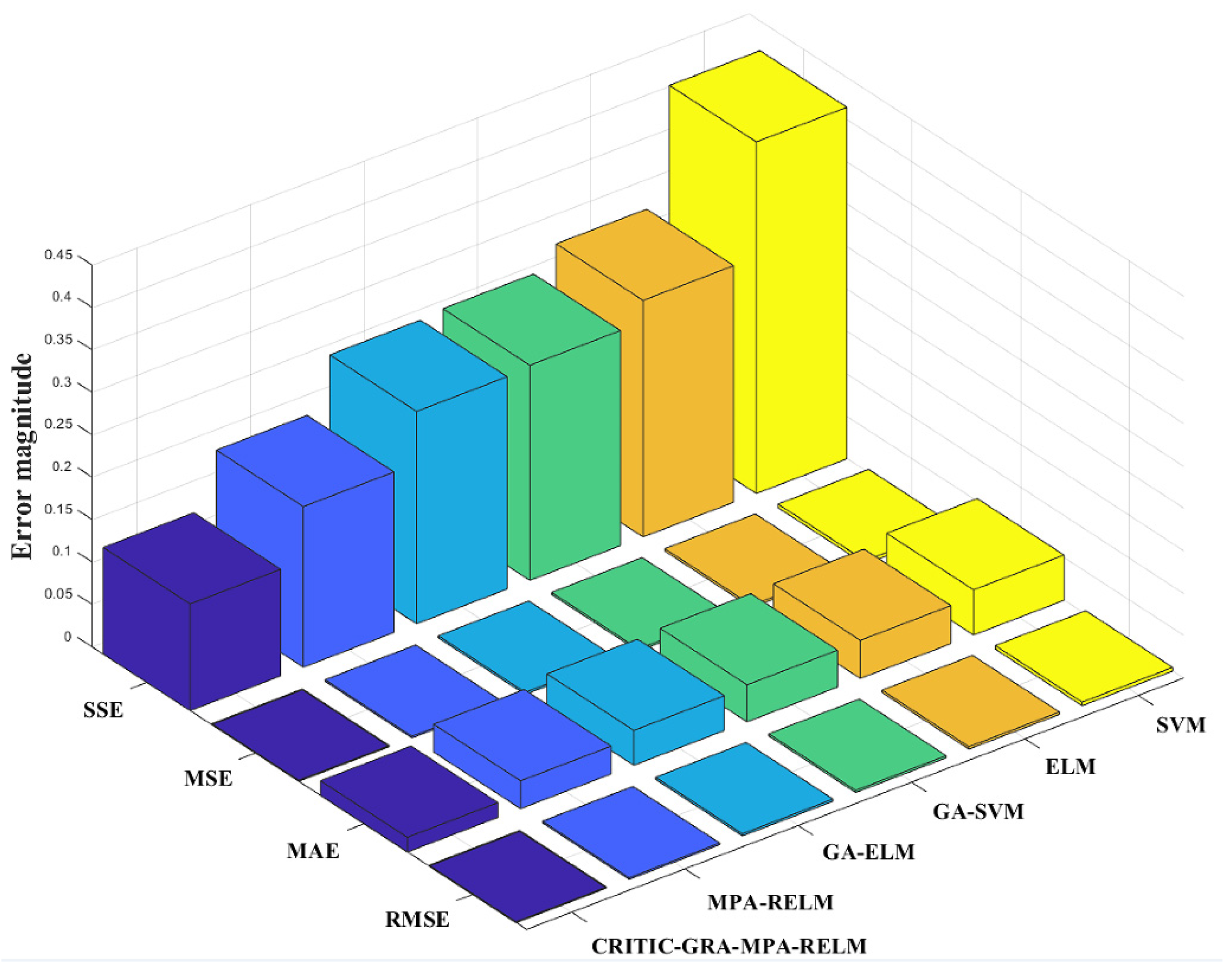
In order to better show the prediction effect of the six models, this paper selects the error indicators SSE, MSE, MAE, and RMSE. The result shows that all the error indicators of the spot market price prediction model constructed in this paper are the lowest, and are better than other models. After screening similar days, the data was further optimized, so that the SSE of the MPA-RELM model was improved by 0.0636, the MSE was improved by 0.0007, the MAE was improved by 0.0154, and the RMSE was improved by 0.0007.

In order to further verify that the prediction model constructed in this paper has more accurate prediction performance, DM test was used to test the significance of the prediction results of MPA-RELM, GA-ELM, GA-SVM, ELM, and SVM, and the p-values of different models are shown in the following table.

According to the prediction effect and prediction deviation of different models in Figure 10, Figure 11 and Figure 12, it shows that the CRITIC-GRA-MAP-RELM model proposed in this paper has strong applicability to the forecast of day-ahead spot electricity prices, and according to the error analysis in

Table 8. Results of various error indicators of different prediction models.

	CRITIC-GRA-MPA-RELM	MPA-RELM	GA-ELM	GA-SVM	ELM	SVM
residual sum of squares (SSE)	0.1257	0.1893	0.2504	0.2536	0.2789	0.4145
mean squared error (MSE)	0.0013	0.0020	0.0026	0.0026	0.0029	0.0043
mean absolute error (MAE)	0.0165	0.0328	0.0411	0.0436	0.0449	0.0533
root mean square error (RMSE)	0.0013	0.0020	0.0026	0.0026	0.0029	0.0043

and the significance analysis in

Table 9. p-values for the Diebold and Mariano test.

p	MPA-RELM	GA-ELM	GA-SVM	ELM	SVM
CRITIC-GRA-MPA-RELM	0.04	0.02	<0.01	<0.01	<0.01

, the fitting effect and error of the forecast model are as follows: CRITIC-GRA-MPA-RELM > MPA-RELM > GA-ELM > GA-SVM > ELM > SVM. From the deviation trend and distribution characteristics of each prediction model, the following conclusions can be further drawn:

(1)

The prediction error of the ELM model is lower than that of the SVM model, indicating that ELM is more adaptable than SVM for electricity price forecasting. From the forecast trend, it can be seen that the electricity price predicted by SVM is generally higher than that of ELM, and the electricity price trend of SVM during the evening peak is opposite to that of ELM, indicating that the SVM forecast curve is more volatile. The basic RELM model used in this paper is a model further optimized on the basis of ELM, which shows that the model proposed in this paper has a certain model foundation and is more suitable for electricity price forecasting than other machine learning algorithms.

(2)

The error of MPA-RELM is lower than that of GA-ELM, indicating that using MPA to optimize RELM can improve the accuracy of machine learning more than the GA model to optimize ELM. The electricity price prediction curve from MPA-RELM is basically the same as that of GA-ELM. The electricity price curve predicted by the MPA-RELM model still has a large deviation, but MPA-RELM reduces the deviation of each time point, especially in the evening peak, meaning MPA-RELM is closer to the real electricity price.

(3)

CRITIC-GRA-MPA-RELM has the highest prediction accuracy, and MPA-RELM is second only to the model proposed in this paper, indicating that further screening of historical data, obtaining historical daily data similar to the market on the forecast day, which can better adapt to the volatility of electricity prices in the spot market, can improve the prediction accuracy of the MPA-RELM model and prevent the model from overfitting.

Through the comparative analysis of the above models, it can be seen that the CRITIC-GRA-MPA-RELM model proposed in this paper is more suitable for spot market electricity price forecasting, and can better reflect the trend of spot market electricity price fluctuations, especially peaks and troughs. It can make up for the shortcomings of RELM and ELM to a certain extent.

From Figure 13, the error trends of different prediction models can be obtained: firstly, the prediction accuracy of different models is different, but the prediction errors of the six models are all larger in the evening peak, and none of the six models currently predict outliers at 10:45 and 22:30, indicating that the forecast of the day-ahead electricity price not only needs to consider the public information of the electricity market, but also needs to consider the main body’s quotation decision plan. Secondly, according to the historical electricity price trend, the morning peak period is relatively stable, the prediction results of the six models are relatively stable, and all have relatively calibrated prediction results. Among the six models, the prediction results of five models are relatively concentrated. The model proposed in this paper is closer to the real history information, indicating that when forecasting the day-ahead spot electricity price, it is necessary to focus on selecting a historical day that is closer to the forecast date.

5. Conclusions

Based on the analysis of the formation mechanism of electricity price in the spot market, this paper constructs the CRITIC-GRA-MPA-RELM model, verifies the model through the spot price before the day of Shanxi spot pilot, and verifies the progressiveness of this model through five models, including MPA-RELM, GA-ELM, GA-SVM, ELM, and SVM. According to the prediction results, the following conclusions are obtained:

(1)

Through the CRITIC-GRA model to screen the original data, the original data structure can be optimized to ensure the accuracy of the input data of the prediction model.

(2)

Through the comparison of several prediction models, it shows that the MPA algorithm has better optimization speed and global search ability than the GA algorithm under the same conditions, and can improve the generalization ability of RELM.

(3)

Combined with the relevant data of Shanxi spot pilot, it is verified that CRITIC-GRA-MPA-RELM can deal with peak and trough electricity prices, and the avoided single model can only deal with the problem of low volatility.

(4)

The forecasting error of the forecasting model proposed in this paper is concentrated in the electricity price spike period, which shows that, when forecasting electricity price, we should not only consider the market public information, but also pay attention to the means of planning.

In the future, on the basis of screening similar days, the probability distribution of electricity price at each time point should be considered to improve the accuracy of the confidence interval of electricity price forecasting. At the same time, according to the peak price and the trough price, the forecast is divided into two levels to ensure the accuracy of the peak price and the trough price forecast, and the non-market-oriented information is used as the correction means of the price forecast.

References

1. Wang, R.; Li, Y. Particle swarm optimization GM(1,2) short-term electricity price prediction method with error correction. Power Syst. Prot. and Contr. 2011, 39, 41–45, 52. [Google Scholar]
2. Zhou, M.; Yan, Z.; Ni, Y.; Li, G. A new method of ARIMA electricity price forecast with error forecast correction. Chin. J. Elec. Eng. 2004, 24, 67–72. [Google Scholar]
3. Jan, F.; Shah, I.; Ali, S. Short-Term Electricity Prices Forecasting Using Functional Time Series Analysis. Energies 2022, 15, 3423. [Google Scholar] [CrossRef]
4. Liu, Y.; Xing, W.; Ding, L.; Xu, Y.; Han, Q.; Wang, Y. Prediction of spot electricity price based on ARIMA-GARCH model. Energy Technol. Econ. 2012, 24, 59–63. [Google Scholar]
5. Billé, A.G.; Gianfreda, A.; del Grosso, F.; Ravazzolo, F. Forecasting electricity prices with expert, linear, and nonlinear models. Int. J. Forecast. 2022. [Google Scholar] [CrossRef]
6. Li, Y. Prediction of electricity market electricity price based on convolutional neural network. Mech. Des. Manuf. Eng. 2021, 50, 101–104. [Google Scholar]
7. Ren, Y. Electricity Price Prediction in Electricity Market Based on Echo State Network. Power Syst. Prot. Control 2016, 44, 111–115. [Google Scholar]
8. Huang, J.; Huang, K.; Xiang, D. Research on multi-regional electricity price prediction based on big data of electricity trading platform. Elec. Appl. 2020, 39, 36–41. [Google Scholar]
9. Hafeez, G.; Islam, N.; Ali, A.; Ahmad, S.; Usman, M.; Saleem Alimgeer, K. A modular framework for optimal load scheduling under price-based demand response scheme in smart grid. Processes 2019, 7, 499. [Google Scholar] [CrossRef] [Green Version]
10. Zheng, J.; Cao, W. Day-ahead electricity price prediction based on GA-ELM neural network. J. Shanghai Elec. Power Univ. 2018, 34, 90–94. [Google Scholar]
11. Wang, H.; Zou, B. Electricity price interval prediction based on dynamic Bayesian network. Power Syst. Prot. Control 2022, 50, 117–127. [Google Scholar]
12. Dong, Y.; Wang, J.; He, J.; Wu, J. Short-term electricity price forecast based on the improved hybrid model. Energ. Convers. Manag. 2011, 52, 2987–2995. [Google Scholar] [CrossRef]
13. Liu, L.; Bai, F.; Su, C.; Ma, C.; Yan, R.; Li, H.; Sun, Q.; Wennersten, R. Forecasting the occurrence of extreme electricity prices using a multivariate logistic regression model. Energy 2022, 247, 123417. [Google Scholar] [CrossRef]
14. Wu, S.; He, L.; Zhang, Z.; Du, Y. Forecast of Short-Term Electricity Price Based on Data Analysis. Math. Prob. Eng. 2021, 2021, 6637183. [Google Scholar] [CrossRef]
15. Haque, S. Short-term (Seven Day Basis) load forecasting of a grid system in Bangladesh using artificial neural network. IOSR J. Electr. Electron. Eng. 2021, 15, 15–25. [Google Scholar]
16. Xiao, C.; Sutanto, D.; Muttaqi, K.M.; Zhang, M.; Dong, Z.Y. Online Sequential Extreme Learning Machine Algorithm for Better Pre-Dispatch Electricity Price Forecasting Grids. IEEE T. Ind. Appl. 2021, 57, 1860–1871. [Google Scholar] [CrossRef]
17. Hafeez, G.; Javaid, N.; Riaz, M.; Ali, A.; Umar, K.; Iqbal, Z. Day ahead electric load forecasting by an intelligent hybrid model based on deep learning for smart grid. In Proceedings of the Conference on Complex, Intelligent, and Software Intensive Systems, Sydney, NSW, Australia, 3–5 July 2019; Springer: Cham, Switzerland, 2019; pp. 36–49. [Google Scholar]
18. Kahawala, S.; de Silva, D.; Sierla, S.; Alahakoon, D.; Nawaratne, R.; Osipov, E.; Jennings, A.; Vyatkin, V. Robust Multi-Step Predictor for Electricity Markets with Real-Time Pricing. Energies 2021, 14, 4378. [Google Scholar] [CrossRef]
19. Vega-Márquez, B.; Rubio-Escudero, C.; Nepomuceno-Chamorro, I.A.; Arcos-Vargas, Á. Use of Deep Learning Architectures for Day-Ahead Electricity Price Forecasting over Different Time Periods in the Spanish Electricity Market. Appl. Sci. 2021, 11, 6097. [Google Scholar] [CrossRef]
20. Lu, X.; Qiu, J.; Lei, G. Scenarios modelling for forecasting day-ahead electricity prices: Case studies in Australia. Appl. Energy 2022, 308, 118296. [Google Scholar] [CrossRef]
21. Deng, J.; Huang, Y.; Song, G. Application of time series model based on non-parametric GARCH in day-ahead electricity price forecasting. Power Grid Tech. 2012, 36, 190–196. [Google Scholar]
22. Hwang, J.S.; Kim, J.-S.; Song, H. Handling Load Uncertainty during On-Peak Time via Dual ESS and LSTM with Load Data Augmentation. Energies 2022, 15, 3001. [Google Scholar] [CrossRef]
23. Kontogiannis, D.; Bargiotas, D.; Daskalopulu, A.; Arvanitidis, A.I.; Tsoukalas, L.H. Error Compensation Enhanced Day-Ahead Electricity Price Forecasting. Energies 2022, 15, 1466. [Google Scholar] [CrossRef]
24. Qiao, W.; Yang, Z. Forecast the electricity price of U.S. using a wavelet transform-based hybrid model. Energy 2020, 193, 116704. [Google Scholar] [CrossRef]
25. Haben, S.; Caudron, J.; Verma, J. Probabilistic Day-Ahead Wholesale Price Forecast: A Case Study in Great Britain. Forecasting 2021, 3, 596–632. [Google Scholar] [CrossRef]
26. Brusaferri, A.; Matteucci, M.; Portolani, P.; Vitali, A. Bayesian deep learning based method for probabilistic forecast of day-ahead electricity prices. Appl. Energy 2019, 250, 1158–1175. [Google Scholar] [CrossRef]
27. Mandal, P.; Haque, A.U.; Meng, J.; Srivastava, A.K.; Martinez, R. A novel hybrid approach using wavelet, firefly algorithm, and fuzzy ARTMAP for day-ahead electricity price forecasting. IEEE Trans. Power Syst. 2013, 28, 1041–1051. [Google Scholar] [CrossRef]
28. Conejo, A.J.; Plazas, M.A.; Espinola, R.; Molina, A.B. Day-ahead electricity price forecasting using the wavelet transform and ARIMA models. IEEE Trans. Power Syst. 2005, 20, 1035–1042. [Google Scholar] [CrossRef]
29. Tan, Z.; Zhang, J.; Wang, J.; Xu, J. Day-ahead electricity price forecasting using wavelet transform combined with ARIMA and GARCH models. Appl. Energy 2010, 87, 3606–3610. [Google Scholar] [CrossRef]
30. Yang, W.; Wang, J.; Niu, T.; Du, P. A hybrid forecasting system based on a dual decomposition strategy and multi-objective optimization for electricity price forecasting. Appl. Energy 2019, 235, 1205–1225. [Google Scholar] [CrossRef]
31. Abedinia, O.; Amjady, N.; Zareipour, H. A New Feature Selection Technique for Load and Price Forecast of Electrical Power Systems. IEEE Trans. Power Syst. 2016, 32, 62–74. [Google Scholar] [CrossRef]
32. Garcia-Martos, C.; Rodriguez, J.; Sanchez, M.J. Forecasting electricity prices by extracting dynamic common factors: Application to the Iberian Market. Iet Gener. Transm. Distrib. 2012, 6, 11–20. [Google Scholar] [CrossRef]
33. Yang, W.; Sun, S.; Hao, Y.; Wang, S. A novel machine learning-based electricity price forecasting model based on optimal model selection strategy. Energy 2021, 238, 121989. [Google Scholar] [CrossRef]
34. Westgaard, S.; Fleten, S.E.; Negash, A.; Botterud, A.; Bogaard, K.; Verling, T.H. Performing price scenario analysis and stress testing using quantile regression: A case study of the Californian electricity market. Energy 2021, 214, 118796. [Google Scholar] [CrossRef]
35. Pham, M.H.; Nguyen, M.N.; Wu, Y.K. A novel short-term load forecasting method by combining the deep learning with singular spectrum analysis. IEEE Access 2021, 9, 73736–73746. [Google Scholar] [CrossRef]
36. Díaz, G.; Coto, J.; Gómez-Aleixandre, J. Prediction and explanation of the formation of the Spanish day-ahead electricity price through machine learning regression. Appl. Energy 2019, 239, 610–625. [Google Scholar] [CrossRef]
37. Lehna, M.; Scheller, F.; Herwartz, H. Forecasting day-ahead electricity prices: A comparison of time series and neural network models taking external regressors into account. Energy Econ. 2022, 106, 105742. [Google Scholar] [CrossRef]
38. Shah, I.; Lisi, F. Forecasting of electricity price through a functional prediction of sale and purchase curves. J. Forecast. 2020, 39, 242–259. [Google Scholar] [CrossRef]
39. Ferr, A.; Certaines, G.D.; Cazelles, J.; Cohet, T.; Farnoosh, A.; Lantz, F. Short-Term Electricity Price Forecasting Models Comparative Analysis: Machine Learning vs. Econometrics. 2021. Available online: https://ideas.repec.org/p/hal/wpaper/hal-03262208.html (accessed on 3 January 2022).
40. Dudek, G.; Peka, P. Pattern similarity-based machine learning methods for mid-term load forecasting: A comparative study. Appl. Soft Comput. 2021, 104, 107223. [Google Scholar] [CrossRef]
41. Srivastava, A.K.; Pandey, A.S.; Elavarasan, R.M.; Subramaniam, U.; Mekhilef, S.; Mihetpopa, L. A Novel Hybrid Feature Selection Method for Day-Ahead Electricity Price Forecasting. Energies 2021, 14, 8455. [Google Scholar] [CrossRef]
42. Nitka, W.; Serafin, T.; Sotiros, D. Forecasting electricity prices: Autoregressive hybrid nearest neighbors (ARHNN) method. Working papers in Management Science (WORMS). In Proceedings of the 21st International Conference, Krakow, Poland, 16–18 June 2021; pp. 312–325. [Google Scholar]
43. Khan, S.; Aslam, S.; Mustafa, I.; Aslam, S. Short-Term Electricity Price Forecasting by Employing Ensemble Empirical Mode Decomposition and Extreme Learning Machine. Forecast 2021, 3, 28. [Google Scholar] [CrossRef]
44. Yang, G.; Du, S.; Duan, Q.; Su, J. Short-term Price Forecasting Method in Electricity Spot Markets Based on Attention-LSTM-mTCN. J. Elec. Eng. Technol. 2022, 17, 1009–1018. [Google Scholar] [CrossRef]
45. Cantillo-Luna, S.; Moreno-Chuquen, R.; Chamorro, H.R.; Riquelme-Dominguez, J.M.; Gonzalez-Longatt, F. Locational Marginal Price Forecasting Using SVR-Based Multi-Output Regression in Electricity Markets. Energies 2022, 15, 293. [Google Scholar] [CrossRef]
46. Shi, W.; Wang, Y.; Chen, Y.; Ma, J. An effective Two-Stage Electricity Price forecasting scheme. Electr. Power Syst. Res. 2021, 199, 107416. [Google Scholar] [CrossRef]
47. Zhao, X.; Shen, B.; Lin, L.; Liu, D.; Yan, M.; Li, G. Residential electricity load forecasting based on fuzzy cluster analysis and LSSVM with optimization by the fireworks algorithm. Sustainability 2022, 14, 1312. [Google Scholar] [CrossRef]
48. Klein, N.; Smith, M.S.; Nott, D.J. Deep Distributional Time Series Models and the Probabilistic Forecasting of Intraday Electricity Prices. arXiv 2020, arXiv:2010.01844. [Google Scholar]
49. Yin, H.; Ding, W.; Chen, S.; Zhang, Z.; Zeng, C.; Meng, A. A day-a-day electricity price forecast for new energy power market with high proportion based on long-short-term memory network-crossover algorithm. Power Grid Technol. 2022, 46, 472–480. [Google Scholar]
50. Zhao, Y.; Wang, X.; Jiang, C.; Zhang, J.; Zhou, Z. Short-term electricity price prediction method based on maximum information coefficient correlation analysis and improved multi-level gated LSTM. Chinese J. Electr. Eng. 2021, 41, 135–146, 404. [Google Scholar]
51. Feng, L.; Li, K. Application of improved CRITIC empowerment method in rockburst grade evaluation. Tianjin Chem. Ind. 2021, 35, 63–64. [Google Scholar]
52. Du, Y.; Yang, X.; Lei, S.; Guo, L.; Cao, B. Research on Green Comprehensive Evaluation Model of Urban Distribution Network Electric Energy Based on CRITIC-Order Relation Analysis Method Combination Weighting. E3S Web Conf. 2021, 233, 01145. [Google Scholar] [CrossRef]
53. Ma, C.; Chen, Y.; Ou, L.; Jiang, K. CRITIC-Based Vertical Collusion Control Quality Prediction Based on the Coupling and Coordination Degrees of Socioenvironmental and Public-Investment Bidding Systems in China. Discrete Dyn. Nat. Soc. 2022, 2022, 4209980. [Google Scholar] [CrossRef]
54. Peng, X.; Krishankumar, R.; Ravichandran, K.S. A novel interval-valued fuzzy soft decision-making method based on CoCoSo and CRITIC for intelligent healthcare management evaluation. Soft Comput. 2021, 6, 4213–4241. [Google Scholar] [CrossRef]
55. Wang, W.; Qi, Y.; Jia, B.; Yao, Y. Dynamic prediction model of spontaneous combustion risk in goaf based on improved CRITIC-G2-TOPSIS method and its application. PLoS ONE 2021, 16, e0257499. [Google Scholar] [CrossRef] [PubMed]
56. Guo, K.; Wang, B. PSO-LSSVM transmission line ice thickness prediction model considering grey relational weights. Elec. Mater. 2022, 1, 15–19, 24. [Google Scholar]
57. Zhang, Y.; Wu, Q.; Hu, J. An Adaptive Learning Algorithm for Regularized Extreme Learning Machine. IEEE Access 2021, 9, 20736–20745. [Google Scholar] [CrossRef]
58. Guo, B.; Bai, Y.; Zhao, Y. Production forecast of cutter suction dredger based on PSO-RELM and its visual aided decision making. Water Transport. Eng. 2021, 9, 147–151. [Google Scholar]
59. Shah, I.; Iftikhar, H.; Ali, S.; Wang, D. Short-term electricity demand forecasting using components estimation technique. Energies 2019, 12, 2532. [Google Scholar] [CrossRef] [Green Version]
60. Fan, Y.; Ren, N.; Tian, G.; Duan, Q. Research on spatiotemporal prediction method of dissolved oxygen in ponds based on DeepAR-RELM. J. Agr. Mach. 2020, 51, 405–412. [Google Scholar]
61. Hu, S.; Cui, D. Runoff prediction based on long-term and short-term memory neural network optimization based on marine predator algorithm. China Rural. Water Resour. Hydropower 2021, 2, 78–82, 90. [Google Scholar]
62. Faramarzi, A.; Heidarinejad, M.; Mirjalili, S.; Gandomi, A.H. Marine Predators Algorithm: A Nature-inspired Metaheuristic. Expert Syst. Appl. 2020, 152, 113377. [Google Scholar] [CrossRef]
Figure 1. Spot market electricity price formation process.
Sustainability 14 07767 g001
Figure 2. Spot prices and related factors.
Sustainability 14 07767 g002
Figure 3. MPA optimizes RELM process.
Sustainability 14 07767 g003
Figure 4. CRITIC-GRA-MPA-RELM price forecasting process.
Sustainability 14 07767 g004
Figure 5. The historical day-ahead spot electricity price from 19 February 2022 to 25 February 2022.
Sustainability 14 07767 g005
Figure 6. Related factors of day-ahead spot market from 19 February 2022 to 25 February 2022. (a) Load data for Unified scheduling; (b) Inter-provincial demand load; (c) New energy output; (d) Thermal power output.
Sustainability 14 07767 g006aSustainability 14 07767 g006b
Figure 7. 25 February 2022 Relevant factors.
Sustainability 14 07767 g007
Figure 8. Sorting of similar day.
Sustainability 14 07767 g008
Figure 9. MPA-RELM electricity price forecast curve on 25 February 2022.
Sustainability 14 07767 g009
Figure 10. Comparison of prediction effects of different prediction models on 25 February 2022.
Sustainability 14 07767 g010
Figure 11. Prediction bias of different prediction models.
Sustainability 14 07767 g011
Figure 12. Error evaluation index results of different prediction models.
Sustainability 14 07767 g012
Figure 13. Prediction error trend of different prediction models.
Sustainability 14 07767 g013