When Offline Stores Reduce Online Returns

Abstract

Among the dark sides of contemporary multi-channel retailing are the vast amounts of product returns, especially in the online channel. High product returns not only put pressure on the retailers’ profitability, but also come at high societal and environmental costs. A central question then is whether multi-channel retailers can use their offline stores to help reduce product returns in the online channel without harming online sales. In an empirical study, we address this issue using data from a large Dutch shoe retailer. We develop a novel spatial model to estimate the influence of proximate retail stores on customers’ online shopping behavior, while controlling for spatial and customer heterogeneity. Results demonstrate that an increased offline channel presence indeed reduces online returns, depending on the product’s risk profile, without significantly lowering online sales. Offline stores can thus be an effective and appealing way for retailers to mitigate the negative impact of online shopping related to product returns.

1. Introduction

1.1. Omnichannel Retailing and Product Returns

In recent years, the retail industry has undergone a profound transformation. Driven by customers, who increasingly shop online, retailers have been expanding to the Internet. For the traditional offline retail giant Wal-Mart, e-commerce has become a strategic pillar, and the websites of once traditional offline retailers H&M, Asos, and Zara are now among the most-visited fashion e-commerce sites [1,2]. This trend is reinforced by the recent COVID-19 pandemic, with, for example, Inditex (Zara, among others) announcing the closure of 1200 physical stores worldwide in favor of its online retailing activities [3]. However, while providing our societies and their citizens with an unprecedented choice, online retailing also has a dark side. A large proportion of the products ordered online are returned to the retailer, with return rates reported to vary between 10% and 50% on average [4,5,6], representing up to USD 761 billion in lost sales in the USA alone [6], which more than doubled from USD 350 billion in 2017 [7].

One option for retailers when deciding what to do with the returned products, is to salvage them through liquidators, thus recovering only a low percentage (10–20% on average [8]) of the actual value. However, a shocking number of these products are simply disposed of as waste, even when not showing any relevant deficiencies. Examples include Nike allegedly destroying intact sports gear [9], and Amazon destroying a wide range of returned products [10]. While a clear financial burden to the retailers, the societal and environmental costs of such disposal may be even higher, both in terms of wasted resources to produce the product, and of the returned product that has become waste which needs to be recycled or even destroyed.

While several strategies are put in place to reduce the amount of returned products (including, for example, adding zoom features and online customer reviews by online retailers; see e.g., [11]), retailers only partly succeed in doing so. Interestingly, a trend emerges in which former online-only retailers have embraced an omni-channel strategy and have begun to open or cooperate with offline stores. Examples are Warby Parker and Allbirds [12], as well as Amazon [13,14]. The latter, after ending its experiment with opening physical stores in different product categories (e.g., “Amazon Books” bookstores, “Amazon Go” convenience stores), now focuses on its “Wholefoods” physical grocery stores [13] and its cooperation with Kohl’s to allow for in-store returns at Kohl’s department stores [14]. Ultimately, retailers and “e-tailers” might converge into a common, omni-channel business model [15,16]. This trend of online-going-offline is the more remarkable given that, in the past decade, traditional offline retailers closed many physical retail stores, a development for which the term “retail apocalypse” has been coined [17]. The opening of and cooperation with physical stores by former online-only retailers, however, indicates that there could actually be clear benefits in a combination of online activities with physical retail stores. Such benefits might lie in the sales revenues from the offline stores, but also in changing customer behavior in the online channel. The question then becomes whether such offline stores of the retailer can help reduce online returns, and if so, whether this can be achieved without reducing online sales.

In this paper, we investigate what effects the physical stores of traditional offline retailers have on customer behavior in their online channel. Online customer behavior pertains to two critical determinants of profitability: (1) the number of product purchases, and (2) the number of product returns [18]. Retailers’ profits will also depend on company-controlled factors like margins, servicing costs, and return handling costs. However, as retailers face more uncertainty on decisions by customers, we will focus on providing insights on how offline presence affects customers’ purchase and return behavior. In other words, what happens to purchases and returns if store presence increases or decreases? Regarding the former, there might be negative effects between the online and offline channel but also positive signaling effects. Regarding the latter, stores might increase returns by making returns easier and cheaper, which would be negative, but they might also decrease returns by allowing customers to ascertain a satisfactory product fit before ordering, which would be positive. Both might be differently affected by offline stores, depending on the performance risk associated with the product. Nearby offline stores might change customer purchase or return behavior only for products which need personal fitting and not products which do not, or only for cheaper products and not for more expensive products.

This study builds on the findings of the previous work on channel additions (e.g., [19,20,21,22,23,24]). First, we adopt a holistic view of the impact of offline store presence on the retailer’s online channel performance by analyzing the impact on online purchase frequency, volume, and product returns. Thereby, we go beyond prior work by [21] in providing insights on the impact of the offline channel on purchases and returns in the online channel. We thus acknowledge that retailers will not only look at a reduction of product returns, but will also look at overall performance and performance growth in terms of sales and resulting profitability. Second, we investigate how products’ risk profiles affect the impact of changes in offline presence on the retailer’s online channel performance. The analyses provide an understanding of where and when cross-channel effects are positive or negative. Third, we investigate the effects of store presence in all national regions instead of store openings in retailer-selected regions. In addition, we propose and use a novel model specification, a hierarchical Spatial Durbin Error Poisson model. We thus incorporate the impact of the historical offline presence of the retailer. In sum, we contribute to prior literature by:

-

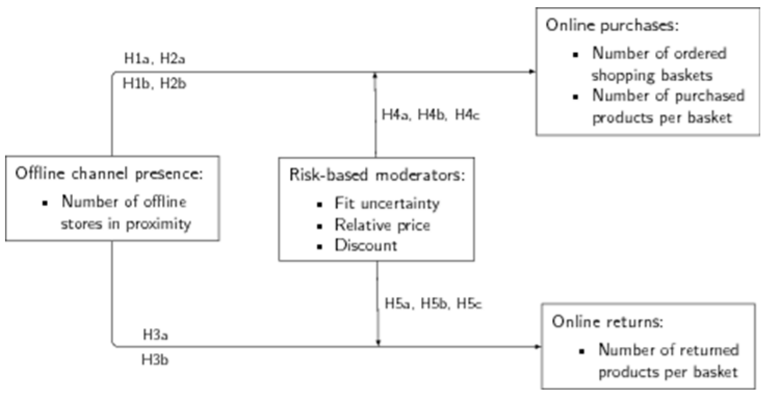
investigating the influence of offline store presence on online purchases (in terms of how often and how much at a time customers order) and returns,

-

integrating how risk-related product characteristics moderate the influence of offline stores presence, and

-

proposing a novel spatial model specification to analyze the effect, avoiding regional selection bias and taking account of the spatial structure of the data.

In our analysis, we use data of 10,000 online customers of a large retailer in the fashion industry, offering a range of products with different characteristics with regard to price and personal fit, over a period of 6 years. Data from this industry are particularly suited, as it is the consumer industry in which e-commerce is most prevalent, with, for example, over two thirds of customers in the European Union shopping online for such products [25]. Moreover, as demonstrated above, large parts of the returned products in this industry are destroyed or dumped (thereby ending up in places like Chile’s Atacama desert [26]), even when no deficiencies are present. As the percentage of e-commerce steadily grows in other product categories, issues that play a role in the fashion sector today might extend to other categories in the future, also given similar return destruction strategies in other categories (see the Amazon example above). In our model section, we develop an extended version of the Spatial Durbin Error Model. This allows us to model the effect of stores on customer behavior while taking into account customer and regional heterogeneity. Moreover, and differing from the models applied in extant research in this matter, it allows us to account for the (extra-)regional influence of stores (i.e., store influence as a function of distance to the customer).

Results of our analyses demonstrate that an increased offline channel presence does not lower the sales in the online channel. However, depending on the products’ risk profiles, it helps the retailer, and thus also society, in reducing product returns. A simulation study demonstrates that reductions in product returns due to increased offline store availability can amount to 4.83–5.65%, depending on the type of product, for moderate increases in the number of offline stores.

1.2. Theoretical Background

Online and offline channels compete with each other along the whole customer journey (i.e., during pre-purchase, purchase, and post-purchase [27]). During the customer journey, customers can interact with multiple channels [28]. For example, many customers visit stores, pre-purchase, and subsequently purchase online (so-called show-rooming), or visit a website, pre-purchase, and subsequently purchase the product in a store (so-called web-rooming). However, channel choices are dependent of each other as channels “affect one another because of lock-in effects, channel inertia, and cross-channel synergies” [29]. Therefore, the availability of one channel influences customer behavior across the whole customer journey and across channels. Concerning the consequences of offline channel availability on purchases and returns in the online channel, there might be multiple, competing processes, which we will describe in this section. The conceptual framework underlying our work is presented in Figure 1.

1.2.1. Purchases

There are two mechanisms of how the availability of one channel can influence purchases in another channel. The first mechanism consists of channel presence leading to channel substitution. The second mechanism, in turn, consists of channel presence having a global promotional effect. Both point to a different effect direction, resulting in two competing hypotheses.

Customers choose channels based on characteristics of the channels, and the ability to fulfil customer preferences; [30] identified six motives for shopping: shopping convenience, information seeking, immediate possession, social interaction, the retail shopping experience, and variety seeking. Different shopping channels are suited to a different extent to comply with these motives. Online shopping may score higher on convenience and variety seeking while offline shopping wins on immediate possession and the retail shopping experience [31,32]. The ranking of the motives and thereby the ranking of the channels depends on personal preference. For example, variety-seeking customers might have a stronger preference for shopping online while social interaction-favoring customers might have a stronger preference for going to a retail store [33]. Thus, the relative weights of the different motives and the resulting preferences will vary between consumers. When channel preference is strong relative to retailer preference, the absence of the preferred channel (e.g., offline) will make consumers shop at competing retailers that do offer a nearby offline option. However, when channel preference is relatively weak and an offline retailer opens an online channel, this may move some of its customers to the online channel (e.g., [20]). The burden of having to travel to a (distant) store is now taken away by the new online channel. However, when that retailer opens a physical store nearby, the relative burden of traveling to a (nearby) store becomes much smaller, possibly tilting the balance in favor of the close offline store instead of the online option. Previous research [23] demonstrating the negative effects of the addition of an offline store on online sales in regions where online sales were relatively high, provides evidence for such mechanisms. At an overall level, across customers, online channel purchases are therefore expected to be lower in the presence of the offline channel, albeit the effects are likely small. Since this could translate to both less frequent orders, i.e., less ordered shopping baskets, and/or smaller orders, i.e., less purchased products per shopping basket, we hypothesize the following:

H1a. 

Offline channel presence decreases the number of ordered shopping baskets.

H2a. 

Offline channel presence decreases the number of purchased products per shopping basket.

On the other hand, stores can also have a promoting function [34] due to their mere presence, and can thus convert non-shoppers in the online channel to shoppers in that channel. Such non-shoppers can be existing customer from the offline channel as well as new customers who used to shop at competitors in the offline channel. Customers can be primed in the need recognition phase by seeing stores of a brand, to visit the web shop of this brand. Moreover, customers can also change channels in a later stage, as is exemplified by the phenomenon of show-rooming. Here, customers deliberately visit a store to choose a product without purchasing it. Instead, they change channels for the actual purchase. Both phenomena could explain why, especially in areas where online sales are relatively low, adding offline stores may thus boost online sales [23]. Next to the promoting function, the offline channel can have a logistics function by allowing customers to order online and pick up the ordered items in a physical store (BOPIS: buy online, pick up in store) [35,36]. Offering such logistics flexibility could further increase the attractiveness of ordering in the online channel. In general, the existence of the offline channel can thus draw customers to make purchases in the online channel. Again, this might result in both more frequent orders, i.e., more ordered shopping baskets, and/or larger orders, i.e., more purchased products per shopping basket. There-fore, we hypothesize the following:

H1b. 

Offline channel presence increases the number of ordered shopping baskets.

H2b. 

Offline channel presence increases the number of purchased products per shopping basket.

1.2.2. Returns

The presence of an offline channel can also influence the number of product returns. As before, we focus on the effect on the online channel (i.e., products returned that were purchased in the online channel). Again, two mechanisms with opposite directionality are at play, resulting in two competing hypotheses.

On one side, the offline channel might decrease returns due to customers’ reaction to perceived risk [37]. According to [38], social, financial, physical, performance, time, and psychological risks can influence consumer behavior. For fashion products, the type of products that we focus on, performance risk is pronounced [39]. For such products, performance is largely determined by product fit (i.e., the match between customer preferences and product properties [40]). The amount of uncertainty concerning product fit depends on channel choice, as offline stores allow for much better inspection of physical products than an online website. Customers can anticipate this increased uncertainty and the resulting increased likelihood of returning and adapt their purchase behavior accordingly [41]. In particular, when offline stores are available, customers can shift the first stages of their decision-making process to offline stores. That is, they would engage in show-rooming to reduce fit uncertainty. For the final purchase, however, consumers may move to the online stores, as they may want to take some time to evaluate the different options before the actual purchase or want to benefit from the convenience of purchases delivered at home. As a result, subsequent returns of such purchases made in the online channel are likely lower. In addition, customers can shift the whole customer journey to the stores, becoming “one-stop shoppers” in the offline channel [33]. Regarding the return rate, results would be the same: customers would return less in the online channel. Therefore, we hypothesize the following:

H3a. 

Offline channel presence decreases the number of returned products per shopping basket.

On the other side, returns might increase due to the decreased “cost” of returning. It has been found that the effort it takes to return a product influences the likelihood that customers actually return a product [42]. The decision to return a product is a result of a cost/benefit calculation. Even though a product might not ideally fit the customer’s preferences, returning the product is associated with a cost. The cost of returning the product must be lower than the shortcoming in the utility of the product in order for a return to be worthwhile [40,43]. When there is no offline channel available, customers must re-package the product in a parcel, label it, drive to a post office, and, sometimes, pay shipping fees. In addition, a refund will usually be offered only after the firm received the product back and checked its condition. On the other hand, when stores are available, customers can simply return the product there, thereby avoiding shipping fees, investment in time and effort, and packaging. In consequence, returning costs for the customer are lower when the offline channel is available. Therefore, the cost/benefit calculation is likely more often in favor of returning and, thus, customers might also return more, leading to the following hypothesis:

H3b. 

Offline channel presence increases the number of returned products per shopping basket.

1.2.3. The Role of Risk

Purchasing a product is generally associated with risk. As argued above, fashion products suffer from performance risk due to uncertainty regarding the fit between product properties and customer preferences [39,40]. However, while all products have some risk, the relative amount of risk differs.

In particular, whether or not a product fits (i.e., its fit uncertainty), depends on the type of product; a first type of fashion product is highly dependent on the customer’s physiology. Such products are generally offered in multiple sizes (e.g., XS, M, XXL) and, by consequence, pre-purchase fit uncertainty is higher. Conversely, a second type of fashion products is mostly independent of the customer’s physiology. Such products are therefore offered only in one size (e.g., bags and watches) and, by consequence, pre-purchase fit uncertainty is lower. Despite technological advances in the online channel (e.g., zoomable product images [11]), customers still need to visit a store and check their personal physiology in combination with the product to eliminate fit uncertainty. When more offline stores are available to customers with a stronger retailer preference compared to the channel preference, customers can more easily reduce fit uncertainty by visiting a store either before ordering online or even instead of ordering online. This will especially be relevant for products with higher levels of fit uncertainty, where customers will more actively look for options to reduce this uncertainty. When customers visit a store before ordering online, fit uncertainty and thereby returns are likely reduced, and when customers visit a store instead of ordering online, both purchases and returns are likely reduced. In sum, we expect offline store availability to have a negative effect on purchases and returns for the online channel for high fit-uncertainty, multi-size products. For purchases and returns of low fit-uncertainty, uni-size products, we expect effects to be limited or even absent.

In addition, performance risk of a product also depends on customers’ expectations. Customers have higher quality expectations for products that are relatively more expensive [44]. For products that are perceived as less expensive (i.e., due to a low price relative to competitors or having a price discount), customers might be more willing to accept slight deficits in the product. Consequently, perceived performance risk is lower for such products. Therefore, customers will feel less of a need to reduce the risk by interacting with the offline channel instead of, or before, interacting with the online channel. However, when perceived performance risk becomes higher, the need to mitigate this risk also becomes stronger, and the availability of ways to do so becomes more salient. While an increase in the number of offline stores may be less relevant for products with a low perceived performance risk, it will be more relevant in the case of products with a high perceived performance risk. In consequence, we expect availability of offline stores to have a negative effect on both purchases and returns in the online channel for (high-risk) undiscounted and relatively higher-priced products. For purchases and returns of (low-risk) discounted and relatively lower-priced products, we expect effects to be limited or even absent. In sum, we expect risk level in regard to fit uncertainty, price level, and discount to moderate the effect of offline channel presence on both purchases and returns (Figure 1). Therefore, we hypothesize that:

H4. 

The impact of offline channel presence on the number of purchased products per shopping basket is more negative/less positive for (a) products with higher fit uncertainty (i.e., multi-size products), (b) higher-priced products, and (c) undiscounted products, compared to products with lower fit uncertainty, lower-priced products, and discounted products, respectively.

H5. 

The impact of offline channel presence on the number of returned products per shopping basket is more negative/less positive for (a) products with higher fit uncertainty (i.e., multi-size products), (b) higher-priced products, and (c) undiscounted products, compared to products with lower fit uncertainty, lower-priced products, and discounted products, respectively.

2. Materials & Methods

2.1. Data

To assess the impact of offline channel availability on the customer purchase and return behavior in the online channel, we conduct an empirical analysis with data from a large Dutch retailer in the fashion segment that sells shoes, bags, belts, socks, wallets, and similar products. We first provide insights on the sample and the definitions of the variables we use in our analyses. We then discuss issues related to invalid cases and missing variables, and provide basic descriptive statistics on the most important variables.

2.1.1. Sample

The dataset at hand contains a sample of 10,000 online customers of the focal retailer who ordered at least one product between 8 September 2008 and 5 October 2014. In total, customers ordered more than 20,000 products (in about 15,000 shopping trips or baskets) and returned more than 3500 products in this period. Orders could be delivered at home or picked up in one of the stores. Generally, for each product order, we have detailed information on the product that was ordered and the customer who ordered it. In a small number of cases, product or customer information is missing and we had to remove the associated orders from the dataset (see section: Invalid Cases and Missing Variables).

The address of the customer serves to assign each customer to one region. The regions are defined using zip-codes (i.e., each region comprises the area which is covered by the same 4-digit zip-code), which leads to relatively small and contiguous regions. This allows us to examine the influence of the retailer’s offline stores on customers’ online shopping behavior while taking proximity into account. The number of stores is rather stable over time, ranging from 405 in 2005 to 430 in 2017, with a peak of 460 in 2012. We gather the location of the retailer’s stores, and the associated zip-code region, from a database of store locations (schoenenwinkelsoverzicht.nl, accessed on 19 May 2017). The average size of a region is 10.900 km² (sd = 20.276 km²).

Using the store location data, we calculate the count of stores within each region plus the count of stores beyond that region and apply spatial decay for the latter (we provide more information on the so-called spatial decay in the Model section) and use these as our explanatory variables.

2.1.2. Variables

For our analysis, we use the following dependent variables, the number of ordered shopping baskets per customer, purchased products per shopping basket, and returned products per shopping basket. Decomposing the total number of purchases and returns into ordered shopping baskets and purchases/returns per shopping baskets has two benefits. First, it allows for separate assessment of (1) how many times customers order, and (2) how much they purchase and return per order. Second, it allows for the addition of order-level control variables to the analysis of (2).

We expect store availability to have a different influence for products of different price levels, discounts, and sizes. Thus, we separately analyze purchases and returns of three pairs of complementing subsets of products, namely the subsets of products with either (1) higher or lower fit uncertainty, (2) with higher or lower price, and (3) without or with a discount. For distinguishing higher- from lower-priced products, we use a within-category median split of undiscounted product prices. Using a within-category split instead of an across-category split is based on the notion that cheap categories can still contain relatively expensive, and thus risky, products and vice versa. In total, we thus have seven sets of products: one set with all products, and three times two complementary sets. For each set, we analyze purchases and returns, resulting in 14 outcome variables (see

Table 1. Product purchase and return variables.

k	Variables	Description
k = 0	purchasesi,c,r,0 returnsi,c,r,0	Number of overall purchased/returned products a
k = 1	purchasesi,c,r,1 returnsi,c,r,1	Number of purchased/returned multi-size products a
k = 2	purchasesi,c,r,2 returnsi,c,r,2	Number of purchased/returned uni-size products a
k = 3	purchasesi,c,r,3 returnsi,c,r,3	Number of purchased/returned products priced above the median price in their category a
k = 4	purchasesi,c,r,4 returnsi,c,r,4	Number of purchased/returned products priced below the median price in their category a
k = 5	purchasesi,c,r,5 returnsi,c,r,5	Number of purchased/returned products without discount a
k = 6	purchasesi,c,r,6 returnsi,c,r,6	Number of purchased/returned products with discount a

^a in shopping basket i of customer c in region r.

).

As control variables, we use demographic information, month and year of the order, and additional regional information like welfare, urbanization, car ownership, and post office locations. The latter originate from Statistics Netherlands (CBS), the Netherlands Institute for Social Research (SCP), and the Dutch post (PostNL), respectively. For post offices, we reverse geo-coded their geographical coordinates to zip-code regions using the ArcGIS services API [45] and included a count with spatial decay as a control variable, similar to our approach of including retail store locations that are also based on zip-code regions.

2.1.3. Invalid Cases and Missing Variables

In some cases, the data contained incomplete or unusable information on ordered products or customers. First, we removed the product orders for which product characteristics were missing, as we cannot estimate the influence of product characteristic-based moderators. Second, we removed product orders, where customers could not be assigned to a region or regional statistical information was not available. In total, we removed 57 full customers (from 10,000 to 9943; i.e., 0.57%), 705 entire shopping baskets (from 15,122 to 14,426; i.e., 4.60%), and 1171 specific product purchases (from 21,360 to 20,189; i.e., 5.48%).

Data on gender and age is only available for a portion of the data (percentage observed: 49.3% for gender and 46.3% for age). Deleting all cases with missing data would dramatically shrink the sample size and hence statistical power [46]. Therefore, for age, we add an additional dummy variable to indicate missing values and set the missing data value itself to the mean of non-missing data. For gender, we only add an additional dummy variable to indicate missing values.

2.1.4. Descriptive Overview

In

Table 2. Variables used in the purchase and return models.

Variable	Description
Customer Behavior
basketsc,r	Number of ordered shopping baskets by customer c in region r
purchasesi,c,r,k	Number of purchased products in shopping basket i of customer c in region r with product characteristic k
returnsi,c,r,k	Number of returned products in shopping basket i of customer c in region r with product characteristic k
Regional characteristics
(W × stores)r	Number of stores in region r and its surrounding regions with spatial decay
(W × posts)r	Number of post offices in region r and its surrounding regions with spatial decay
welfarer	welfare indicator a for region r
urbanizationr	urbanization indicator a for region r
carsr	cars per capita a in region r
Order characteristics
yeari	Year in which the order i was made (0 = 2008, …, 6 = 2014), accounting for a linear trend
month2,i, …, month12,i	11 indicators for the month in which order i was made (baseline: January), accounting for seasonal effects
Customer characteristics
agec	Age of customer c in years a
genderc	Customer c is female (1) or male (0)

^a mean-centered.

, we present a description of all variables included in our analysis. In total, we observe 14,426 ordered shopping baskets by 9943 customers. A customer orders on average 1.451 shopping baskets (sd = 1.044; range 1–18). A shopping basket contains on average 1.399 purchased products (sd = 0.826; range 1–17) and 0.251 returned products (sd = 0.649; range 0–10). Customers identified predominantly as female (86.63% of the observed gender) and were 40.524 years on average (sd = 11.314). The average number of stores of our retailer per region is 0.121 (sd = 0.594; range 0–12).

2.2. Methodology

We first present the base model specifications for the three focal outcome variables in our analyses (i.e., number of ordered shopping baskets per customer, number of purchased products in a shopping basket, and number of returned products in a shopping basket). Next, we introduce the Spatial Durbin Error model specification for these models to account for spatial dependence across regions. We end this section with insights on the estimation procedure.

2.2.1. Base Model Specifications

We employ three hierarchical spatial regression models to estimate the effects of store availability. First, we estimate a model for the number of shopping baskets ordered by a customer over the period of observation, dependent on the number of stores in proximity, in addition to several other control variables, including the customer’s age and gender, to account for customer heterogeneity. We account for distance by pre-multiplying a weighting matrix W to the vectors stores and posts. This operation adds to the two variables the spatially decayed (i.e., diminished) values of neighboring regions. By that, a higher number of stores in one region also increases the number of stores in proximate regions, but to a lesser extent the higher the distance between both regions. The further two regions A and B are apart, the less the stores of region A will count in the total store value of region B (and vice versa). Furthermore, we add a regional error term for unobserved regional heterogeneity. Since proximate regions are more similar to each other than distant regions, we permit spatial auto-correlation in the regional error term; the closer the regions are, the stronger they will resemble each other, and the more they will be correlated. In the subsection “Spatial Durbin Error Model”, we describe the spatial aspect of our model in more detail. We assume a zero-truncated Poisson distribution for the dependent variable, because all customers in the sample order at least once. The resulting, first model is presented in Equation (1):

$$\begin{array}{cc}\hfill basket{s}_{c,r}& |\sim ztPoisson\left(exp({\mu }_{basket{s}_{c,r}})\right)\hfill \\ \hfill {\mu }_{basket{s}_{c,r}}& |={\alpha }_1+{\beta }_{1}ag{e}_c+{\beta }_{2}gende{r}_c\hfill \\ \hfill & |+{\theta }_{1}welfar{e}_r+{\theta }_{2}urbanisatio{n}_r+{\theta }_{3}car{s}_r\hfill \\ \hfill & |+{\gamma }_1{\left(W\times stores\right)}_r+{\gamma }_2{\left(W\times posts\right)}_r \hfill \\ \hfill & |+u_r\hfill \\ \hfill u_r=& ({I_J-{\lambda }_k{W}_u)}^{-1}{\epsilon }_r,{\epsilon }_r\sim N\left(0,{\tau }_k\right)\hfill \end{array}$$

(1)

Second, we estimate a model for the number of purchased products per shopping basket, as illustrated in (2). We estimate the same model for all purchases_i,c,r,k variables presented in Table 1. For purchases_i,c,r,0 we assume a zero-truncated Poisson distribution, since all baskets contain at least one product of any sort, and for the remaining orders variables we assume a regular Poisson distribution. We account for observed customer heterogeneity by including age and gender in the model, and add a customer-level random effect to account for further unobserved heterogeneity.

$$\begin{array}{cc}\hfill purchase{s}_{i,c,r,0}& |\sim ztPoisson\left(exp\left({\mu }_{purchase{s}_{i,c,r,0}}\right)\right),\hfill \\ \hfill purchase{s}_{i,c,r,k}& |\sim Poisson\left(exp\left({\mu }_{purchase{s}_{i,c,r,k}}\right)\right) \forall k\in \left\{2, 7\right\},\hfill \\ \hfill {\mu }_{purchase{s}_{i,c,r,k} }& |={\alpha }_{1,k}+{\beta }_{1,k}yea{r}_i+{\displaystyle {\displaystyle \sum }_{m=2}^{12}}{\beta }_{2.m,k}mont{h}_{m,i}\hfill \\ \hfill & |+{\beta }_{3,k}ag{e}_c+{\beta }_{4,k}gende{r}_c\hfill \\ \hfill & |+{\theta }_{1,k}welfar{e}_r+{\theta }_{2,k}urbanisatio{n}_r+{\theta }_{3,k}car{s}_r\hfill \\ \hfill & |+{\gamma }_{1,k}{\left(W\times stores\right)}_r+{\gamma }_{2,k}{\left(W\times posts\right)}_r \hfill \\ \hfill & |+{\epsilon }_{c,k}+u_{r,k},\hfill \\ \hfill {\epsilon }_{c,k}\sim N(0,{\mathsf{\sigma }}_k),& u_{r,k}={(I_J-{\lambda }_k{W}_u)}^{-1}{\epsilon }_{r,k},{\epsilon }_{r,k}\sim N\left(0,{\tau }_k\right).\hfill \end{array}$$

(2)

Third, we estimate a model for the number of returned products per shopping basket, as illustrated in Equation (3). We estimate the same model separately for all returns_i,k variables provided in Table 1, and we always assume a regular Poisson distribution for the dependent variable. Similar to before, we control for regional and customer heterogeneity as well as year and month:

$$\begin{array}{cc}\hfill return{s}_{i,k}& |~ Poisson\left(exp\left({\mu }_{return{s}_{i,k}}\right)\right)\hfill \\ \hfill {\mu }_{return{s}_{i,k}}& |={\alpha }_{1,k}+{\beta }_{1,k}purchase{s}_i\hfill \\ \hfill & |+{\beta }_{2,k}yea{r}_i+{\displaystyle {\displaystyle \sum }_{m=2}^{12}}{\beta }_{3.m,k}mont{h}_{m,i}\hfill \\ \hfill & |+{\beta }_{4,k}ag{e}_c+{\beta }_{5,k}gende{r}_i\hfill \\ \hfill & +{\theta }_{1,k}welfar{e}_r+{\theta }_{2,k}urbanisatio{n}_r+{\theta }_{3,k}car{s}_r\hfill \\ \hfill & |+{\gamma }_{1,k}{\left(W\times stores\right)}_r+{\gamma }_{2,k}{\left(W\times posts\right)}_r\hfill \\ \hfill & |+{\epsilon }_{c,k}+u_{r,k},\hfill \\ \hfill {\epsilon }_{c,k}\sim N(0,{\mathsf{\sigma }}_k),u_{r,k}& ={(I_J-{\lambda }_k{W}_u)}^{-1}{\epsilon }_{r,k},{\epsilon }_{r,k}\sim N\left(0,{\tau }_k\right).\hfill \end{array}$$

(3)

In sum, we use separate models to identify whether a customer (a) orders more often (i.e., more shopping baskets), (b) purchases more products at a time (i.e., more products per shopping basket), and/or (c) returns more products per shopping basket. This allows us to assess consumer behavior in more detail than only estimating a model of total product purchases/returns and conflating order frequency and quantity.

2.2.2. Spatial Durbin Error Model

In our models, we use both spatial predictors and a spatial error term. The use of spatial predictors follows the idea that “responses by individuals are […] correlated in such a manner that individuals near one another in the space generate similar outcomes” [47] (p. 268). More formally, an observed outcome of unit A does not only depend on characteristics of entity A, but also on characteristics of neighboring entity B, C and so on. This is called spatial dependence. Spatial models reflect that process by incorporating the influence of neighboring entities into the regression equation, weighted by a metric of their distances. The use of a spatial error term follows the idea that spatially situated observations are influenced more or less by the same unobservable factors (e.g., infrastructure; culture), depending on their distance to each other. This would normally lead to heteroskedasticity in the error term, but can be dealt with by a spatial model, by explicitly modelling autocorrelated errors. Using both spatial predictors and a spatial error term is called the Spatial Durbin Error model [48]. In its most basic form, it looks as follows:

$$\begin{array}{cc}\hfill & \mathrm{Y}|=X_A\beta +W{X}_B\theta +u, \hfill \\ \hfill \mathrm{with}: & u|=\lambda Wu+\epsilon ,\hfill \\ \hfill & \epsilon |\sim N\left(0,{\sigma }^2{I}_n\right)\hfill \end{array}$$

The dependent variable Y_i of observation i is influenced by the independent variables in X_A belonging to the same observation i and a linear combination of independent variables in X_B of possibly all other observations, through pre-multiplying the data vector or matrix with the square weighting matrix W. Thus, how neighbors influence each other is defined by the matrix W. The weighting matrix W is also used to model the autocorrelation between error terms (u = λWu).

We modify this model to estimate both own-region and cross-region effects with θ by including the diagonal in W. Furthermore, we restrict the parameter range of λ to a maximum of one by scaling the matrix W used in the formula to calculate u [49].

The resulting matrices are:

$$W \mathrm{with} W_{i,j}=\left\{\begin{array}{c}{e}^{-\frac{2}{10}{D}_{i,j}},|e^{-\frac{2}{10}{D}_{i,j}}>10\%\\ 0,|otherwise\end{array},\right.$$

$$W_u{}_{ }=\frac{1}{v-1} \left(W-I\right)$$

with D_i,j being the distance between i and j and v the largest eigenvalue of W. We assume an exponential decay with a cut-off at an influence of less than 10%, which corresponds to D_i,j > 11.5 km. A cut-off value is necessary to generate a sparser matrix and make computation more efficient. For D_i,j, we use the linear distance between the centroids of each zip-code region.

The Spatial Durbin Error model is the preferred spatial model when modelling local spillover effects [50,51]. However, the model illustrated above has some limitations we need to address. First, the model is non-hierarchical, which makes it unsuitable for most marketing applications. We therefore add a second level to the model, thereby building on the work by [52]. Such a second hierarchy level allows for expression of the nesting of multiple customers within one spatial region. As illustrated above, we coalesce regional effect within- and beyond-region effects so that we have one parameter estimate per regional influential factor. Second, to be able to estimate effects on discrete (instead of continuous) outcomes, we use a Poisson (or zero-truncated Poisson) distribution instead of a Normal distribution. Since multivariate count distributions have a range of issues with regards to theoretical feasibility, computability, and interpretability, with no generally agreed-upon solution (see e.g., [53]), we model the influences on each dependent variable separately, using a (zero-truncated) univariate Poisson distribution for each of the resulting hierarchical Spatial Durbin Error Poisson models.

2.2.3. Estimation

We use a Bayesian approach to obtain the estimates for the models. Such an approach offers flexibility in tailoring the models to the specific requirements of the topic at hand (e.g., [49] (p. 124), and at the same time accommodates the hierarchical structure of the error terms in our models (e.g., [52]). In particular, we use the No-U-Turn Markov Chain Monte Carlo sampling (NUTS) provided by the Stan software package [54]. We use uninformative (uniform) priors for all parameters. The error structure of the model requires computing the inverse of a function of the spatial weighting matrix W at each sampling step. The high number of regions and the resulting high dimensionality of the spatial weight matrix, however, renders this computationally unfeasible. Instead, we approximate the inverse by a Neumann series. When estimating, all relevant parameters of all models converged, with their so-called potential scale reduction factor (PSRF or $\widehat{\mathrm{R}}$) being smaller than 1.1. We also tested the model by simulating data and comparing the true to the estimated parameters. Here as well, results were satisfying. Finally, we checked for multicollinearity among the explanatory variables. All VIF scores are well below the critical value of 5 [55], with a highest value of 4.13, confirming that the models do not suffer from multicollinearity. More details on simulation, model estimation, and convergence can be found in the Appendix A.

3. Results

We first share some model-free insights, and then report the model-based results on the influence of offline stores on the number of shopping baskets customers order online. Next, we present the influence of stores on the number of purchased and returned products per shopping basket, when including all products. Finally, we report the influence of stores on purchases and returns per shopping basket for complementing subsets of products, namely based on price level, discounting, or size.

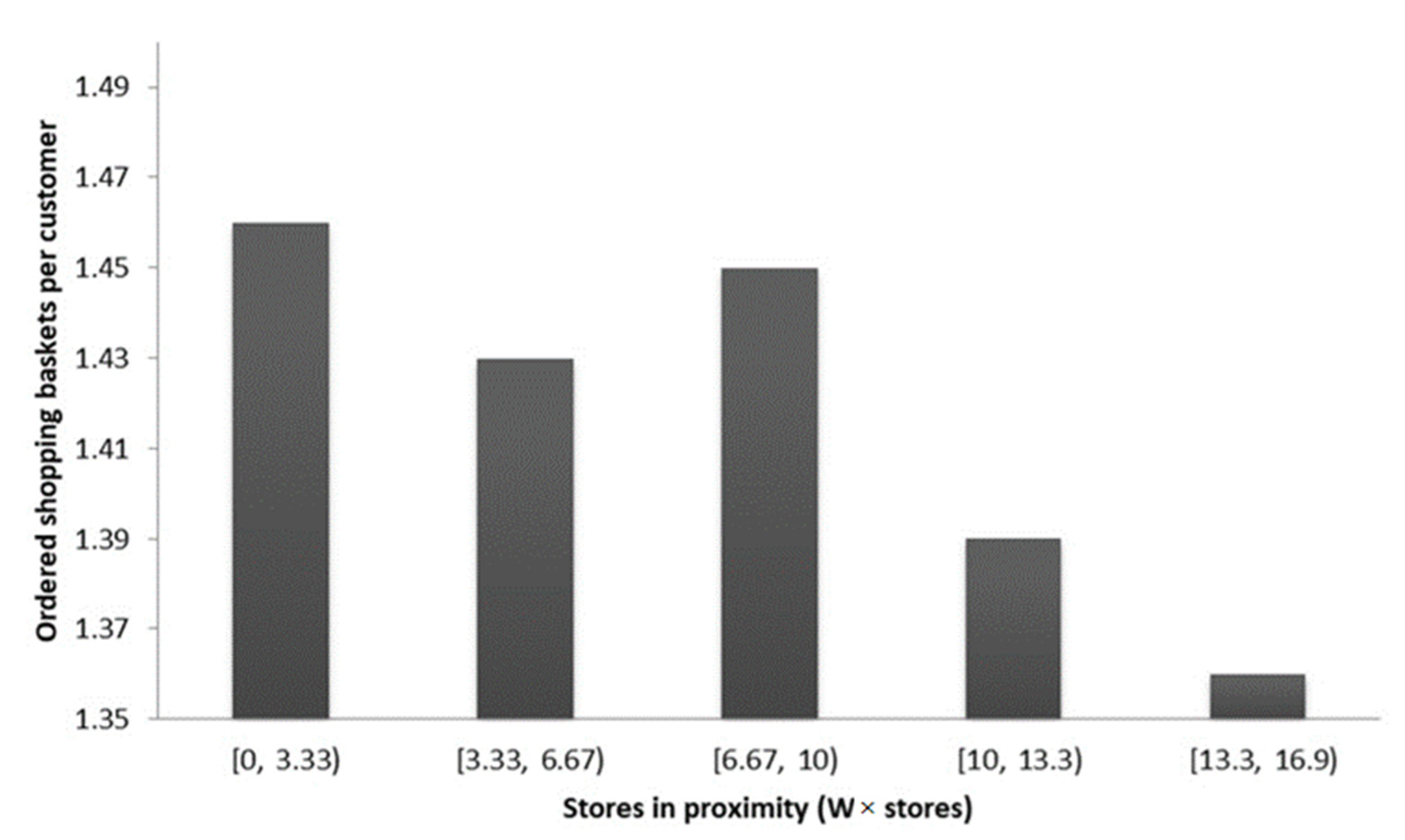
3.1. Model-Free Insights

Figure 2 illustrates that the number of ordered baskets is relatively equal for lower numbers of stores in proximity (1.46, 1.43, and 1.45), but then drops for the higher numbers of stores in proximity (1.39 and 1.36). However, overall, there is little to no evidence of a significant effect, with the correlation between the number of ordered shopping baskets and number of stores in proximity being small and insignificant (−0.017, p > 0.10).

The number of purchases per shopping basket also appears to become lower for the higher numbers of stores in proximity (

Table 3. Number of purchases and returns per basket for different numbers of stores in proximity and the associated correlation.

Stores in Proximity (W × stores):	[0, 3.33)	[3.33, 6.67)	[6.67, 10)	[10, 13.3)	[13.3, 16.9)	Correlation
Purchases:
Overall	1.39	1.41	1.45	1.41	1.07	0.015
Multi-size	1.33	1.36	1.41	1.34	1.07	0.022 **
Uni-size	0.06	0.05	0.04	0.07	0.00	−0.024 **
Price above median	0.89	0.80	0.82	0.93	0.67	−0.047 ***
Price below median	0.51	0.61	0.63	0.48	0.40	0.060 ***
Undiscounted	1.00	0.99	1.04	1.13	1.00	0.015
Discounted	0.39	0.42	0.41	0.27	0.07	0.000
Returns:
Overall	0.28	0.21	0.19	0.16	0.00	−0.064 ***
Multi-size	0.27	0.20	0.19	0.16	0.00	−0.062 ***
Uni-size	0.01	0.01	0.00	0.00	0.00	−0.018 *
Price above median	0.18	0.13	0.11	0.12	0.00	−0.063 ***
Price below median	0.10	0.07	0.08	0.04	0.00	−0.025 **
Undiscounted	0.20	0.14	0.13	0.15	0.00	−0.060 ***
Discounted	0.08	0.07	0.06	0.02	0.00	−0.027 **
Observations	9688	3510	1048	165	15

*** p < 0.001, ** p < 0.01, * p < 0.05.

), although this picture is not constant across product types with different risk levels. Overall, across all product types, there is no evidence of a significant effect, with the correlation between the number of purchases per shopping basket and the number of stores in proximity being insignificant (0.015, p > 0.10). The number of returns per shopping basket, on the other hand, demonstrates a negative relation with the number of stores in proximity, for both overall and all product types with different risk levels. The strongest correlations can be found for the higher-risk product types: multi-size products (−0.062, p < 0.001), products priced above the median in their category (−0.063, p < 0.001), and products without discount (−0.060, p < 0.001).

3.2. Ordered Shopping Baskets

Table 4 presents the estimation results for the model explaining the number of ordered shopping baskets per customer. The availability of offline stores of the retailer does not help or harm the online channel, as it does not significantly influence the number of ordered shopping baskets (−0.046, 95% credibility interval (CI: −0.127, 0.032)). Thus, we find no empirical support for H1a or H1b.

Regarding demographic control variables, customers with a higher age order more (0.003, CI: 0.000, 0.007) and customers who do not disclose their age or gender order less (−0.250, CI: −0.319, −0.180; and −1.215, CI: −1.312, −1.113, respectively). Regional control variables are generally insignificant at the 5% level, with the exception of car ownership (0.213, CI: 0.019, 0.390). There is significant heterogeneity at the regional level (0.572, CI: 0.527, 0.619) and significant spatial auto-correlation (0.335, CI: 0.010, 0.857).

Table 4. Regional influence on the number of ordered shopping baskets.

DV	Basketsc
Intercept	−0.002	(−0.061, 0.056)
(W × Stores)r	−0.046	(−0.127, 0.032)
Regional control variables
(W × posts)r	0.066	(−0.013, 0.146)
welfarer	−0.000	(−0.038, 0.039)
urbanizationr	−0.008	(−0.048, 0.033)
carsr	0.223	(0.019, 0.390) *
Customer control variables
gender_manc	−0.065	(−0.160, 0.027)
gender_missingc	−1.215	(−1.312, −1.113) ***
agec	0.003	(0.000, 0.007) *
age_missingc	−0.250	(−0.319, −0.180) ***
Random effects and spatial autocorrelation
τ (random effect region)	0.572	(0.527, 0.619) ***
λ (spatial auto-correlation)	0.335	(0.010, 0.857) ***

Numbers in brackets indicate the 95% credible interval (CI) and stars indicate whether the 95% (*), 99% (**), 99.9 (***) CI excludes zero.

Table 4. Regional influence on the number of ordered shopping baskets.

DV	Basketsc
Intercept	−0.002	(−0.061, 0.056)
(W × Stores)r	−0.046	(−0.127, 0.032)
Regional control variables
(W × posts)r	0.066	(−0.013, 0.146)
welfarer	−0.000	(−0.038, 0.039)
urbanizationr	−0.008	(−0.048, 0.033)
carsr	0.223	(0.019, 0.390) *
Customer control variables
gender_manc	−0.065	(−0.160, 0.027)
gender_missingc	−1.215	(−1.312, −1.113) ***
agec	0.003	(0.000, 0.007) *
age_missingc	−0.250	(−0.319, −0.180) ***
Random effects and spatial autocorrelation
τ (random effect region)	0.572	(0.527, 0.619) ***
λ (spatial auto-correlation)	0.335	(0.010, 0.857) ***

Numbers in brackets indicate the 95% credible interval (CI) and stars indicate whether the 95% (*), 99% (**), 99.9 (***) CI excludes zero.

3.3. Purchases and Returns per Shopping Basket

Table 5. Regional influences on the general number of purchases and returns (per shopping basket) in the online channel.

DV	Purchasesi		Returnsi
Intercept	−2.000	(−2.193, −1.817) ***	−2.879	(−3.111, −2.652) ***
(W × stores)r	−0.039	(−0.101, 0.024)	−0.127	(−0.216, −0.038) **
Regional control variables
(W × posts)r0	0.068	(0.012, 0.126) *	−0.059	(−0.140, 0.022)
welfarer	−0.027	(−0.058, 0.002)	−0.015	(−0.056, 0.025)
urbanisationr	0.012	(−0.021, 0.045)	−0.061	(−0.106, −0.016) *
carsr	0.222	(0.065, 0.375) **	−0.437	(−0.749, −0.143) **
Customer control variables
gender_manc	−0.024	(−0.136, 0.088)	−0.511	(−0.682, −0.346) ***
gender_missingc	−0.244	(−0.333, −0.157) ***	−0.320	(−0.434, −0.206) ***
agec	0.000	(−0.004, 0.005)	0.003	(−0.003, 0.009)
age_missingc	0.033	(−0.056, 0.128)	0.158	(0.040, 0.275) **
Order control variables
ordersi	n.a.		0.572	(0.543, 0.600) ***
yeari	0.197	(0.165, 0.230) ***	0.075	(0.034, 0.115) ***
monthi,2	0.037	(−0.149, 0.222)	−0.135	(−0.345, 0.073)
monthi,3	0.383	(0.235, 0.536) ***	0.058	(−0.128, 0.241)
monthi,4	0.487	(0.339, 0.633) ***	0.028	(−0.148, 0.201)
monthi,5	0.459	(0.316, 0.602) ***	−0.000	(−0.179, 0.178)
monthi,6	0.496	(0.349, 0.645) ***	0.109	(−0.073, 0.287)
monthi,7	0.687	(0.548, 0.833) ***	−0.271	(−0.453, −0.082) **
monthi,8	0.479	(0.332, 0.628) ***	−0.233	(−0.428, −0.041) *
monthi,9	0.315	(0.171, 0.464) ***	−0.438	(−0.628, −0.249) ***
monthi,10	0.427	(0.278, 0.575) ***	−0.238	(−0.429, −0.050) **
monthi,11	0.130	(−0.047, 0.298)	−0.073	(−0.280, 0.122)
monthi,12	0.406	(0.241, 0.562) ***	−0.151	(−0.356, 0.044)
Random effects and spatial autocorrelation
σ (random effect customer)	0.736	(0.698, 0.776) ***	0.785	(0.723, 0.850) ***
τ (random effect region)	0.056	(0.003, 0.144) ***	0.196	(0.034, 0.325) ***
λ (spatial auto-correlation)	0.492	(0.030, 0.973) ***	0.585	(0.041, 0.986) ***

Numbers in brackets indicate the 95% credible interval (CI) and stars indicate whether the 95% (*), 99% (**), 99.9 (***) CI excludes zero.

presents the estimation results for the models explaining the number of purchases and returns per shopping basket. Again, we find no evidence that the availability of offline stores helps or harms the online channel in terms of purchased products per shopping basket, as it does not significantly influence the number of purchased products per shopping basket (−0.039, CI: −0.101, 0.024). Therefore, we find no support for H2a or H2b. However, the availability of offline stores has a beneficial effect on returns per shopping basket as it significantly decreases the number of returned products per shopping basket (−0.127, CI: −0.216, −0.038), which is empirical evidence for H3a (and against H3b).

Regarding control variables, men return less than women do (−0.511, CI: −0.682, −0.346) and customers who do not disclose their gender have both fewer purchases and returns (−0.511, CI: −0.682, −0.346; and −0.320, CI: −0.434, −0.206, respectively). Conversely, customers who do not disclose their age return more (0.158, CI: 0.040, 0.275). Both purchases and returns increase over time (0.197, CI: 0.165, 0.230; and 0.075, CI: 0.034, 0.115, respectively). Several regional control variables have a significant effect, as well: post office availability increases purchases (0.068, CI: 0.012, 0.126), car ownership increases purchases (0.222, CI: 0.065, 0.375) and decreases returns (−0.437, CI: −0.749, −0.143), and urbanization decreases returns (−0.061, CI: −0.106, −0.016). For both purchases and returns, there is significant spatial auto-correlation (0.492, CI: 0.030, 0.973; and 0.585, CI: 0.041, 0.986, respectively), and significant heterogeneity on the customer (0.736, CI: 0.698, 0.776; and 0.785, CI: 0.723, 0.850, respectively) and regional level (0.056, CI: 0.003, 0.144; and 0.196, CI: 0.034, 0.325, respectively).

3.4. Influence of Risk

Table 6 presents the estimation results for the models explaining the number of purchases and returns per shopping basket for the subsets of products with multiple sizes (multi-size) and the with one size (uni-size). The availability of offline stores does not significantly harm purchases in the online channel of products of either subset (−0.015, CI: −0.041, 0.012; and 0.126, CI: −0.034, 0.281, respectively). Thus, we find no support for H4a. However, the availability of offline stores does have a beneficial influence on product returns as it reduces the number of returns per shopping basket of multi-size products (−0.123, CI: −0.212, −0.037). In line with our reasoning, it has no significant influence on returns of uni-size products (−0.365, CI: −1.147, 0.395). Thus, we find support for H5a.

Table 7 illustrates the estimation results for the models, explaining the number of purchases and returns per shopping basket for the subsets of lower- and higher-price products, respectively. As before, the availability of offline stores has no significant harmful effect for either set of products in terms of number of purchases (−0.018, CI: −0.069, 0.034; and −0.006, CI: −0.041, 0.031 respectively). Thus, we find no empirical evidence for H4b. However, the availability of offline stores again has a beneficial effect by decreasing returns per shopping basket in the case of more expensive products (−0.132, CI: −0.240, −0.029) and, as argued, it has no significant influence on returns of cheaper products (−0.127, CI: −0.283, 0.028). Thus, we find support for H5b.

Table 8 presents the estimation results for the models explaining the number of purchases and returns per shopping basket for the subsets of discounted and undiscounted products. The influence of offline store availability on purchases/returns of discounted and undiscounted products is in line with the effect of store availability on purchases/returns of cheaper and more expensive products. That is, the availability of offline stores has no significant influence on purchases of both discounted products and undiscounted products (0.001, CI: −0.060, 0.064; and −0.009, CI: −0.039, 0.022, respectively). Thus, we find no support for H4c. Similar to before, the availability of offline stores decreases returns of undiscounted products (−0.153, CI: −0.249, −0.057) while, however, not affecting returns of discounted products (−0.068, CI: −0.237, 0.096). Thus, we find support for H5c.

3.5. Simulation of Effect Magnitude

Translating the coefficient estimates reported above to actual effects sizes is a non-trivial exercise, since the models we use to calculate the effects of store availability on orders and returns are non-linear. Therefore, in this section, we present the results of using partly simulated data to predict the outcome variable in order to find out what change in the number of stores leads to what reduction in returned products per shopping basket. We restrict the prediction to the models where the effect of stores was significant. Therefore, the predictions pertain to the influence of stores on the number of returned products per shopping basket, regarding all products as well as regarding multi-size, higher-priced, and undiscounted products.

Table 6. Regional influences on online purchasing and returning (per shopping basket) for uni-size products vs. multi-size products.

	Uni-Size Products		Multi-Size Products
DV	Purchasesi	Returnsi	Purchasesi	Returnsi
Intercept	−3.572 ***	−8.908 ***	−0.074	−2.902 ***
(W × stores)r	0.126	−0.365	−0.015	−0.123 **
Regional control variables
(W × posts)r	−0.150 *	−0.234	0.028 *	−0.060
welfarer	0.062	−0.119	−0.011	−0.013
urbanisationr	−0.150 ***	0.141	0.010	−0.068 **
carsr	−0.010	−0.716	0.087 *	−0.475 ***
Customer control variables
gender_manc	−0.956 ***	−0.893 *	0.016	−0.513 ***
gender_missingc	−0.010		−0.082 ***	−0.319 ***
agec	−0.003	−0.053 *	0.000	0.004
age_missingc	−0.067	0.571	0.014	0.151 *
Order control variables
purchasesi	n.a.	3.045 ***	n.a.	0.596 ***
yeari	0.013	−0.133	0.057 ***	0.077 ***
monthi,2	0.243	−1.701	−0.022	−0.124
monthi,3	−0.105	0.577	0.111 **	0.048
monthi,4	−0.611 **	0.505	0.152 ***	0.007
monthi,5	0.087	0.502	0.127 ***	−0.016
monthi,6	−0.116	0.750	0.147 ***	0.088
monthi,7	−0.285	−0.439	0.249 ***	−0.285 **
monthi,8	0.052	0.621	0.148 ***	−0.252 *
monthi,9	−0.081	0.260	0.090 *	−0.460 ***
monthi,10	−0.418 *	−0.005	0.124 ***	−0.243 *
monthi,11	0.321	0.070	0.019	−0.077
monthi,12	0.711 ***	−0.246	0.056	−0.133
Random effects and spatial autocorrelation
σ (random effect customer)	1.254 ***	2.149 ***	0.010 ***	0.780 ***
τ (random effect region)	0.117 ***	0.627 ***	0.010 ***	0.203 ***
λ (spatial auto-correlation)	0.506 ***	0.499 ***	0.500 ***	0.601 ***

Stars indicate whether the 95% (*), 99% (**), 99.9 (***) CI excludes zero. Missing and male gender dummies have been collapsed due to low case count for returns of uni-size products.

Table 6. Regional influences on online purchasing and returning (per shopping basket) for uni-size products vs. multi-size products.

	Uni-Size Products		Multi-Size Products
DV	Purchasesi	Returnsi	Purchasesi	Returnsi
Intercept	−3.572 ***	−8.908 ***	−0.074	−2.902 ***
(W × stores)r	0.126	−0.365	−0.015	−0.123 **
Regional control variables
(W × posts)r	−0.150 *	−0.234	0.028 *	−0.060
welfarer	0.062	−0.119	−0.011	−0.013
urbanisationr	−0.150 ***	0.141	0.010	−0.068 **
carsr	−0.010	−0.716	0.087 *	−0.475 ***
Customer control variables
gender_manc	−0.956 ***	−0.893 *	0.016	−0.513 ***
gender_missingc	−0.010		−0.082 ***	−0.319 ***
agec	−0.003	−0.053 *	0.000	0.004
age_missingc	−0.067	0.571	0.014	0.151 *
Order control variables
purchasesi	n.a.	3.045 ***	n.a.	0.596 ***
yeari	0.013	−0.133	0.057 ***	0.077 ***
monthi,2	0.243	−1.701	−0.022	−0.124
monthi,3	−0.105	0.577	0.111 **	0.048
monthi,4	−0.611 **	0.505	0.152 ***	0.007
monthi,5	0.087	0.502	0.127 ***	−0.016
monthi,6	−0.116	0.750	0.147 ***	0.088
monthi,7	−0.285	−0.439	0.249 ***	−0.285 **
monthi,8	0.052	0.621	0.148 ***	−0.252 *
monthi,9	−0.081	0.260	0.090 *	−0.460 ***
monthi,10	−0.418 *	−0.005	0.124 ***	−0.243 *
monthi,11	0.321	0.070	0.019	−0.077
monthi,12	0.711 ***	−0.246	0.056	−0.133
Random effects and spatial autocorrelation
σ (random effect customer)	1.254 ***	2.149 ***	0.010 ***	0.780 ***
τ (random effect region)	0.117 ***	0.627 ***	0.010 ***	0.203 ***
λ (spatial auto-correlation)	0.506 ***	0.499 ***	0.500 ***	0.601 ***

Stars indicate whether the 95% (*), 99% (**), 99.9 (***) CI excludes zero. Missing and male gender dummies have been collapsed due to low case count for returns of uni-size products.

The simulation is based on the actual observed data, with the exception of store availability. We base our simulation as closely as possible on the actual data in order to obtain estimates that reflect, as closely as possible, what would happen in a real-world situation, when changing only store availability, meaning we keep almost the entire database used in the analyses intact, but only modify the data on store availability. Next, we predict the outcome variables for each observation using the estimation results presented in the previous subsections. A more stylized example would allow for more freedom with regards to the assumed customer, product, and regional structure but would also suffer from arbitrariness because many different plausible configurations are conceivable, thus lowering the external validity.

Table 7. Regional influences on online purchasing and returning products (per shopping basket) priced below or above the median price.

	Products Priced below Median		Products Priced above Median
DV	purchasesi	returnsi	purchasesi	returnsi
Intercept	−1.034 ***	−4.035 ***	−0.547 ***	−3.414 ***
(W × stores)r	−0.018	−0.127	−0.006	−0.132 *
Regional control variables
(W × posts)r	0.044	−0.060	0.002	−0.063
welfarer	0.019	−0.029	−0.029 ***	0.011
urbanisationr	0.052 ***	−0.052	−0.023 **	−0.055 *
carsr	0.106	−0.375	0.113 **	−0.557 ***
Customer control variables
gender_manc	0.157 ***	−0.476 ***	−0.135 ***	−0.502 ***
gender_missingc	−0.094 **	−0.355 ***	−0.058 *	−0.263 ***
agec	−0.005 **	−0.001	0.003 *	0.004
age_missingc	0.076	0.086	−0.027	0.183 **
Order control variables
purchasesi	n.a.	0.824 ***	n.a.	0.895 ***
yeari	0.038 **	0.044	0.065 ***	0.078 **
monthi,2	−0.119	−0.247	0.070	−0.102
monthi,3	−0.250 ***	0.116	0.294 ***	−0.039
monthi,4	0.026	0.217	0.196 ***	−0.076
monthi,5	0.293 ***	0.413 **	−0.005	−0.208
monthi,6	0.471 ***	0.541 ***	−0.174 ***	−0.021
monthi,7	0.724 ***	0.181	−0.404 ***	−0.434 ***
monthi,8	0.428 ***	−0.104	−0.156 ***	−0.244 *
monthi,9	−1.201 ***	−1.816 ***	0.493 ***	−0.484 ***
monthi,10	−0.994 ***	−1.149 ***	0.488 ***	−0.245 *
monthi,11	−0.487 ***	−0.272	0.294 ***	−0.079
monthi,12	−0.150 *	−0.185	0.243 ***	−0.150
Random effects and spatial autocorrelation
σ (random effect customer)	0.464 ***	1.088 ***	0.022 ***	0.742 ***
τ (random effect region)	0.114 ***	0.210 ***	0.025 ***	0.226 ***
λ (spatial auto-correlation)	0.599 ***	0.511 ***	0.516 ***	0.518 ***

Stars indicate whether the 95% (*), 99% (**), 99.9 (***) CI excludes zero.

Table 7. Regional influences on online purchasing and returning products (per shopping basket) priced below or above the median price.

	Products Priced below Median		Products Priced above Median
DV	purchasesi	returnsi	purchasesi	returnsi
Intercept	−1.034 ***	−4.035 ***	−0.547 ***	−3.414 ***
(W × stores)r	−0.018	−0.127	−0.006	−0.132 *
Regional control variables
(W × posts)r	0.044	−0.060	0.002	−0.063
welfarer	0.019	−0.029	−0.029 ***	0.011
urbanisationr	0.052 ***	−0.052	−0.023 **	−0.055 *
carsr	0.106	−0.375	0.113 **	−0.557 ***
Customer control variables
gender_manc	0.157 ***	−0.476 ***	−0.135 ***	−0.502 ***
gender_missingc	−0.094 **	−0.355 ***	−0.058 *	−0.263 ***
agec	−0.005 **	−0.001	0.003 *	0.004
age_missingc	0.076	0.086	−0.027	0.183 **
Order control variables
purchasesi	n.a.	0.824 ***	n.a.	0.895 ***
yeari	0.038 **	0.044	0.065 ***	0.078 **
monthi,2	−0.119	−0.247	0.070	−0.102
monthi,3	−0.250 ***	0.116	0.294 ***	−0.039
monthi,4	0.026	0.217	0.196 ***	−0.076
monthi,5	0.293 ***	0.413 **	−0.005	−0.208
monthi,6	0.471 ***	0.541 ***	−0.174 ***	−0.021
monthi,7	0.724 ***	0.181	−0.404 ***	−0.434 ***
monthi,8	0.428 ***	−0.104	−0.156 ***	−0.244 *
monthi,9	−1.201 ***	−1.816 ***	0.493 ***	−0.484 ***
monthi,10	−0.994 ***	−1.149 ***	0.488 ***	−0.245 *
monthi,11	−0.487 ***	−0.272	0.294 ***	−0.079
monthi,12	−0.150 *	−0.185	0.243 ***	−0.150
Random effects and spatial autocorrelation
σ (random effect customer)	0.464 ***	1.088 ***	0.022 ***	0.742 ***
τ (random effect region)	0.114 ***	0.210 ***	0.025 ***	0.226 ***
λ (spatial auto-correlation)	0.599 ***	0.511 ***	0.516 ***	0.518 ***

Stars indicate whether the 95% (*), 99% (**), 99.9 (***) CI excludes zero.

Table 8. Regional influences on online purchasing and returning (per shopping basket) for undiscounted vs. discounted products.

	Discounted Products		Undiscounted Products
DV	Purchasesi	Returnsi	Purchasesi	Returnsi
Intercept	−4.059 ***	−5.814 ***	0.354 ***	−3.128 ***
(W × stores)r	0.001	−0.068	−0.009	−0.153 **
Regional control variables
(W × posts)r	−0.029	−0.113	0.036 *	−0.042
welfarer	−0.039 *	−0.018	0.003	−0.006
urbanisationr	0.045 **	−0.094 *	−0.014	−0.055 *
carsr	0.092	−0.607 *	0.074	−0.294
Customer control variables
gender_manc	−0.245 ***	−0.845 ***	0.071 *	−0.449 ***
gender_missingc	−0.260 ***	−0.440 ***	0.008	−0.271 ***
agec	0.001	0.008	−0.000	0.002
age_missingc	0.055	0.203	−0.019	0.142 *
Order control variables
purchasesi	n.a.	0.940 ***	n.a.	0.775 ***
yeari	0.405 ***	0.278 ***	−0.053 ***	0.055 **
monthi,2	0.489 ***	0.429	−0.114 *	−0.307 *
monthi,3	1.210 ***	0.642 **	−0.283 ***	0.009
monthi,4	0.980 ***	0.601 **	−0.099 *	0.033
monthi,5	1.076 ***	0.360	−0.161 ***	−0.047
monthi,6	0.493 ***	0.470 *	0.052	0.021
monthi,7	0.532 ***	−0.458	0.161 ***	−0.377 ***
monthi,8	0.378 ***	−0.106	0.093 *	−0.287 **
monthi,9	1.296 ***	−0.010	−0.356 ***	−0.406 ***
monthi,10	1.123 ***	0.042	−0.169 ***	−0.158
monthi,11	0.924 ***	0.437	−0.196 ***	−0.048
monthi,12	1.191 ***	0.295	−0.212 ***	−0.125
Random effects and spatial autocorrelation
σ (random effect customer)	0.766 ***	1.200 ***	0.014 ***	0.736 ***
τ (random effect region)	0.069 ***	0.146 ***	0.013 ***	0.224 ***
λ (spatial auto-correlation)	0.500 ***	0.504 ***	0.501 ***	0.563 ***

Stars indicate whether the 95% (*), 99% (**), 99.9 (***) CI excludes zero.

Table 8. Regional influences on online purchasing and returning (per shopping basket) for undiscounted vs. discounted products.

	Discounted Products		Undiscounted Products
DV	Purchasesi	Returnsi	Purchasesi	Returnsi
Intercept	−4.059 ***	−5.814 ***	0.354 ***	−3.128 ***
(W × stores)r	0.001	−0.068	−0.009	−0.153 **
Regional control variables
(W × posts)r	−0.029	−0.113	0.036 *	−0.042
welfarer	−0.039 *	−0.018	0.003	−0.006
urbanisationr	0.045 **	−0.094 *	−0.014	−0.055 *
carsr	0.092	−0.607 *	0.074	−0.294
Customer control variables
gender_manc	−0.245 ***	−0.845 ***	0.071 *	−0.449 ***
gender_missingc	−0.260 ***	−0.440 ***	0.008	−0.271 ***
agec	0.001	0.008	−0.000	0.002
age_missingc	0.055	0.203	−0.019	0.142 *
Order control variables
purchasesi	n.a.	0.940 ***	n.a.	0.775 ***
yeari	0.405 ***	0.278 ***	−0.053 ***	0.055 **
monthi,2	0.489 ***	0.429	−0.114 *	−0.307 *
monthi,3	1.210 ***	0.642 **	−0.283 ***	0.009
monthi,4	0.980 ***	0.601 **	−0.099 *	0.033
monthi,5	1.076 ***	0.360	−0.161 ***	−0.047
monthi,6	0.493 ***	0.470 *	0.052	0.021
monthi,7	0.532 ***	−0.458	0.161 ***	−0.377 ***
monthi,8	0.378 ***	−0.106	0.093 *	−0.287 **
monthi,9	1.296 ***	−0.010	−0.356 ***	−0.406 ***
monthi,10	1.123 ***	0.042	−0.169 ***	−0.158
monthi,11	0.924 ***	0.437	−0.196 ***	−0.048
monthi,12	1.191 ***	0.295	−0.212 ***	−0.125
Random effects and spatial autocorrelation
σ (random effect customer)	0.766 ***	1.200 ***	0.014 ***	0.736 ***
τ (random effect region)	0.069 ***	0.146 ***	0.013 ***	0.224 ***
λ (spatial auto-correlation)	0.500 ***	0.504 ***	0.501 ***	0.563 ***

Stars indicate whether the 95% (*), 99% (**), 99.9 (***) CI excludes zero.

With regards to the store availability variable, we use two scenarios of reducing and two scenarios of increasing store availability, in addition to the as-is scenario of actual observed store availability. We deliberately include both increase and decrease scenarios to provide a full picture of the impact of store availability on product returns. We created all scenarios based on what would be plausible from a managerial perspective( i.e., closure of the least promising stores versus opening of most promising stores based on the regional online client-to-store ratio). The underlying rationale is that stores in regions with high online client-to-store ratios will likely have the highest influence on online returns and, therefore, it is most beneficial to open such stores first (and close them last). Conversely, stores in regions with low online client-to-store rations will likely have a small influence on online returns and, therefore, it is beneficial to close such stores first (and open them last). In order to facilitate comparisons, we use the same (absolute) changes in store numbers for opening and closure scenarios.

Table 9. Scenarios used in the simulation.

Scenario	Change in No. Stores	Description
Moderate store reduction	−109	Closure of one store in each region which has a below-median client/store ratio
Modest store reduction	−51	Closure of one store in each region with a client/store ratio in the lowest quartile
As-is store availability	±0	Actual store availability as observed in the data
Modest store increase	+51	Opening of one store per region, ranked by high to low (prospective) client/store ratio until the same number of stores are opened which were closed in the “Modest store reduction” scenario
Moderate store increase	+109	Opening of one store per region, ranked by high to low (prospective) client/store ratio until the same number of stores are opened which were closed in the “Moderate store reduction” scenario

lists all scenarios and the associated changes in store availability in detail.

The results of the simulation demonstrate that both store openings and closures can have a large effect on product returns (Figure 3). The effect sizes greatly depend on how many stores are opened or closed. In general, both the retailer and society will benefit more from store openings in terms of reduced returns than they suffer from store closures in terms of increases in returns. For example, a modest store increase reduces returns by 2.41–2.81%, while a modest store reduction only increases returns by 1.59–1.94%. This asymmetric effect results from stores with likely greatest positive influence being opened first (in the opening scenarios) and being closed last (in the closure scenarios). The effect size varies slightly between product subsets with smallest effect sizes for multi-size products and largest effect sizes for undiscounted products. Figure 3 provides a detailed account of all effects for each scenario and product subset.

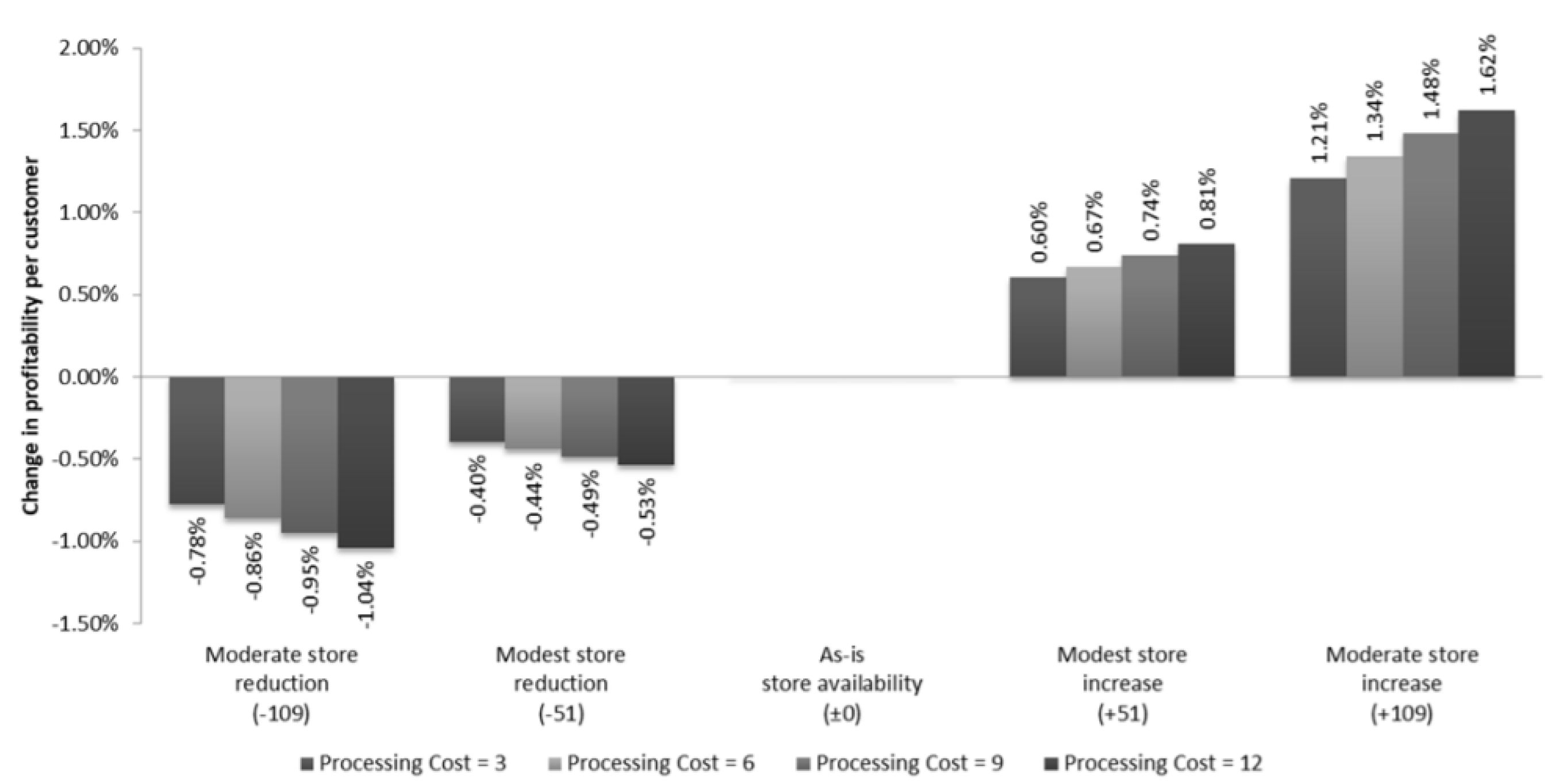
3.6. Profit Implications

While the previous simulation results provide insights on the impact of store openings and closures on product returns, they do not yet illustrate profit implications, which are most relevant for retailers. We therefore simulate the individual-customer profit impact of the different store opening and closure scenarios. We calculate this change based on the following components:

• Return cost per basket, defined as (number of returns per basket) × (return processing cost per return).
• Gross profit per basket, defined as (gross margin × price of an ordered product) × (number of ordered products per basket-number of product returns per basket)
• Profit per customer, defined as (gross profit per basket-return cost per basket) × (number of ordered baskets per customer).

We base our calculations on a gross margin of 42.5% (as reported by [56]), and a return processing cost of EUR 3 to EUR 12, based on interactions with practitioners from online retailing. We use the profit per customer in the existing situation as a benchmark, and determine the percentage change relative to the benchmark scenario. Figure 4 provides a detailed overview of the outcomes for the different scenarios and return processing costs.

The results demonstrate that store openings have a clear beneficial effect on individual-customer profitability. Not surprisingly, this effect is stronger when return processing costs are higher. Moderate store increases could then increase the individual-customer profitability with over 1.6% (processing cost of €12), compared to the existing situation. A same-size decrease in the number of stores, however, would result in a decrease of the individual-customer profitability with over 1%. In the world of online retail, where net profits are often small (if any), these changes, while small, can make the difference for the retailer.

4. Discussion

4.1. Summary of Findings

In this paper, we studied the effect of physical, offline, retail stores on the number of product purchases and product returns by customers in the retailer’s online channel. The results are partly in line with what we predicted (

Table 10. Overview of the main findings.

Hypothesis		Findings
H1a	Offline channel presence decreases the number of ordered shopping baskets.	Not supported
H1b	Offline channel presence increases the number of ordered shopping baskets.	Not supported
H2a	Offline channel presence decreases the number of purchased products per shopping basket.	Not supported
H2b	Offline channel presence increases the number of purchased products per shopping basket.	Not supported
H3a	Offline channel presence decreases the number of returned products per shopping basket.	Supported
H3b	Offline channel presence increases the number of returned products per shopping basket.	Not supported
H4a	The impact of offline channel presence on the number of purchased products per shopping basket is more negative/less positive for products with higher fit uncertainty compared to products with lower fit uncertainty	Not supported
H4b	The impact of offline channel presence on the number of purchased products per shopping basket is more negative/less positive for higher-priced products compared to lower-priced products	Not supported
H5a	The impact of offline channel presence on the number of returned products per shopping basket is more negative/less positive for products with higher fit uncertainty compared to products with lower fit uncertainty	Supported
H5b	The impact of offline channel presence on the number of returned products per shopping basket is more negative/less positive for higher-priced products compared to lower-priced products	Supported
H5c	The impact of offline channel presence on the number of returned products per shopping basket is more negative/less positive for undiscounted products compared to discounted products	Supported

).

Our key result is that offline retail stores contribute to the reduction of returns in the online channel, while not harming the sales of the online channel. Relative to the latter, theory indicates two possible mechanisms through which physical, offline, stores could influence online product purchases: by detracting customers from the online channel due to channel substitution (e.g., [33]), and by attracting customers to the online channel due to cross-channel promotion [34] and logistics services [35,36]. Our findings suggest that both effects are rather small and/or stay in balance.

When it comes to the former, the reduction in the number of returned products per shopping basket as a result of an increased presence of physical stores appears to be most outspoken for products that show a higher perceived risk for customers. These findings are in line with what we theorized. Customers appear to anticipate the risk of needing to return and adapt their purchase behavior, especially for higher-risk products [38,41]. They thus seem to engage in show-rooming for those higher-risk products in order to avoid product returns [33]. Products with multiple sizes, a higher price, or no discount have a higher perceived risk for customers than uni-size, lower-priced, or discounted products. It should therefore not come as a surprise that for the former types of products, physical, offline, stores do reduce product returns, whereas for the latter, lower risk products, offline stores have no significant effect. We find no empirical evidence for an increase in product returns, which could have been fueled by the decreased hassle or cost of actually returning a product [42].

Findings of prior research regarding the influence of offline stores on the online channel are mixed: [21] find that adding physical stores does not cannibalize purchases in the online channel, while [19], in turn, find that adding physical stores does not influence purchases in the online channel in the short run, but does increase them in the long run. Our findings are consistent with the findings by [21], as we find no evidence for a difference in online purchases due to a higher offline store presence. A reason for the difference in findings compared to the study by [19] might be that the retailer in our study is large and well-known so that stores did not increase brand awareness, which was suggested as an explanation for the positive effect in their study. If there would be a positive effect of offline stores on online orders, it would in fact strengthen the notion that stores are helpful and not harmful to the online channel.

Regarding product returns, [21] find that adding physical stores does increase the total return frequency. Their findings, however, are across all channels, and do not distinguish between returns of products purchased online versus offline. Therefore, it is not possible to directly compare our study with their study. Besides, one explanation of the difference might be the higher number of nearby stores in our study. When the retailer has an offline channel but stores are very distant, stores might be attractive enough for customers to use for returning but not attractive enough to use for casual show-rooming, thus fostering returns instead of averting them.

Our study is the first to investigate the influence of the offline channel on purchases and returns in the online channel, which distinguishes between effects for products with different risk perceptions for the customer. Our findings demonstrate that the investigated risk-perception driving product characteristics are a decisive factor for offline-on online-channel influence, and that neglecting them masks an important aspect in the relationship between both channels. Furthermore, we developed a statistical model that takes the regional nature of stores into account and demonstrated that the estimation of a spatial model in this case is feasible, even for a large number of regions. By that, we contribute to prior research on multi-channel interactions, both substantially as well as methodologically, and provide useful and relevant insights on how marketing instruments can mitigate negative impacts of consumer behavior.

4.2. Managerial Implications

Over the course of the last decades, customers shop more and more online, which led to the rise of e-commerce companies, such as Amazon, and the creation of online channels by traditional retailers, such as Wal-Mart. A downside of this increase in online shopping is the ever-increasing amount of returned products, with additional negative environmental consequences due to transportation and a major part of these products ending up as waste. Retailers consequently are challenged to find (profitable) ways to reduce these returns, and the question then is whether offline physical stores can play a role in this. Our findings indicate that physical, offline, stores decrease returns and thereby help to increase the performance of the online channel, which often suffers from high return rates [57]. Also, online sales are not significantly lowered by the presence of an offline store.

The usefulness of physical stores, however, depends on the retailer’s profile and strategy. The retailer’s assortment determines how much overall reduction of product returns in the online channel can be expected. The higher the risk of non-fit for the customer or the more expensive the products on display are, the more returns are reduced. That means retailers that sell higher price products, products without many discounts, and products that have personal fit requirements, stand to benefit the most from physical retail stores.

Furthermore, our simulation demonstrates that the effects of small increases and decreases in the number of stores are asymmetric, with an increase in stores leading to a stronger reduction in returns compared to the increase in returns that results from a similar reduction in the number of stores. This indicates that retailers, and society as a whole, likely benefit from accounting for online customer locations when setting store locations. While a small reduction in the number of, from the point of view of the online channel: unappealing–stores, as a consequence, may not harm the retailer and society much with regard to product returns; a small increase in the number of, from the point of view of the online channel: appealing–stores, will help more. Besides, increasing store availability demonstrates diminishing returns (i.e., adding a few stores has a higher average per-store effect on product returns than adding many stores). That means that gains, per-store, are highest at the first additional store openings. Thus, in general, determining a suitable new store location is not only relevant for offline sales, but also for online sales and product returns.

An important caveat for managers is the fact that, in our analyses, we make abstraction of any costs related to the opening and subsequent operations of offline stores. While our profit simulation demonstrated the individual-customer profit implications of opening (and closing) of stores for online customers, costs incurred (saved) by the retailer to actually open (close) and operate stores were not accounted for. The feasibility of the described strategies will ultimately depend on the opening and operational costs of the offline stores as well as profits made in these stores, and may vary across locations.

4.3. Limitations and Further Research Directions

In our research, we use online data from a fashion retailer. According to [25], clothes and sports goods are the most popular product category for online purchases. Household goods, various media products (books, films, and games), and electronic equipment are the next popular. All these categories differ in their perceived risk for the customer. Therefore, the effect of physical stores on purchases and returns in the online channel might be different. For example, electronic equipment such as televisions usually have a high price and so the effect of physical stores on returns in the online channel might be even more pronounced. A future study could examine the effect of physical stores on purchases and returns for other product categories. In addition, as we only have data on the online channel, we limit our study to investigate the influence of physical stores on online purchases and returns. A future study could integrate offline customer behavior and examine the effect of stores on the combined online and offline purchases and returns.

In addition, we focus our analysis on the within-firm influence of the offline channel on online shopping behavior since firms can directly influence the existence of their own stores. Nevertheless, there could be cross-firm cross-channel influences. Usually, higher switching costs, lock-in effects, sometimes voluntarily set up such as loyalty programs [58], and an assortment of differences impede customers from switching easily from one firm to another [29,59]. In spite of this, one could imagine, for example, a cross-firm category promotion effect. In sum, a future study could investigate the influence of competitor store presence on online purchase and return behavior.

Stores might also have a more or less pronounced promotional and trust-building effect, depending on the retailer. Due to this, we theorized that physical stores could actually increase online sales. While we found no significant effect, this might be due to the fact that our data comes from a large and well-known retailer. In contrast, for smaller and less well-known retailers, this effect might play a role in fostering online purchases [19]. A future study could investigate different retailers and find out under which conditions such a cross-channel promotion effect exists.

Not all stores will offer the same type of advantages to consumers that were offered by the focal retailer in this study (e.g., trying on other sizes, cross-shopping etc.). Moreover, to some retailers, such advantages may be completely irrelevant. Future research could investigate the extent to which investing in increasing the number of return-collection points instead of opening offline stores could be a sound alternative option.

The current setup makes abstraction of the focal retailer’s, as well as competitors’, marketing actions for both the online and offline channels. Such actions include, for example, the assortment offered, advertising effort, as well as applied pricing strategies. A future study could investigate the impact of both the effort of a single retailer in the online relative to the offline channel, and the relative competitive effort of a retailer in the online and/or offline channel on customers’ online purchasing and returning behavior.

Finally, our research took a retailer focus, and concentrated on overall insights on factors retailers can influence. However, taking a consumer focus, an in-depth investigation on role of consumers’ shopping motivations and personality traits could provide valuable insights on multichannel shopping and returning behavior at the consumer level. Next, these insights could be used to design marketing instruments, mitigating some of the negative societal and environmental consequences of multichannel retailing.

References

1. Deloitte. Global Powers of Retailing 2022 Resilience Despite Challenges; Deloitte Touche Tohmatsu Limited: New York, NY, USA, 2022; pp. 1–52. [Google Scholar]
2. Coppola, D. Leading Fashion and Apparel Websites Worldwide 2022, Based on Visit Share. Statista. 19 April 2022. Available online: https://www.statista.com/statistics/1255963/most-visited-fashion-and-apparel-websites/ (accessed on 19 May 2022).
3. Jolly, J. Zara Owner to Close up to 1200 Fashion Stores around the World. The Guardian. 10 June 2020. Available online: https://www.theguardian.com/business/2020/jun/10/zara-owner-to-close-up-to-1200-fashion-stores-around-the-world (accessed on 19 May 2022).
4. Geiger Smith, E. How Online Retailers Predict Your Perfect Outfit. The Wall Street Journal. 5 August 2015. Available online: https://www.wsj.com/articles/how-online-retailers-predict-your-perfect-outfit-1438794462 (accessed on 19 May 2022).
5. Zalando. Returns at Zalando. Zalando. 17 June 2022. Available online: https://corporate.zalando.com/en/newsroom/en/stories/returns-zalando (accessed on 19 May 2022).
6. National Retail Federation. Customer Returns in the Retail Industry 2021. National Retail Federation. 25 January 2022. Available online: https://cdn.nrf.com/sites/default/files/2022-01/Customer%20Returns%20in%20the%20Retail%20Industry%202021.pdf (accessed on 19 May 2022).
7. Mazareanu, E. Costs of Return Deliveries in the United States in 2017 and 2020. Statista. 9 February 2021. Available online: https://www.statista.com/statistics/871365/reverse-logistics-cost-united-states/ (accessed on 19 May 2022).
8. Stock, J.H.; Speh, T.; Shear, H. Managing Product Returns for Competitive Advantage. MIT Sloan Manag. Rev. 2006, 48, 57–62. [Google Scholar]
9. Anne, K.; Rohrbeck, F.; Salewski, C. Schmutziger Fussabdruck. Zeit.de. 11 November 2021. Available online: https://www.zeit.de/2021/46/nike-sneaker-turnschuhe-recycling-muell-modeindustrie-sneakerjagd (accessed on 19 May 2022).
10. Minter, A. Those Amazon Returns? They’re Killing the Environment. Los Angeles Times. 13 November 2019. Available online: https://www.latimes.com/business/story/2019-11-13/amazon-returns-are-killing-the-environment (accessed on 19 May 2022).
11. Minnema, A.; Bijmolt, T.H.; Gensler, S.; Wiesel, T. To Keep or Not to Keep: Effects of Online Customer Reviews on Product Returns. J. Retail. 2016, 92, 253–267. [Google Scholar] [CrossRef]
12. Rosen, E. Online Brands Try a Traditional Marketing Strategy: Physical Stores. The New York Times. 23 March 2022. Available online: https://www.nytimes.com/2022/03/23/business/direct-consumer-retail-stores.html (accessed on 19 May 2022).
13. Dastin, J. Amazon to Shut Its Bookstores and Other Shops as Its Grocery Chain Expands. Reuters. 3 March 2022. Available online: https://www.reuters.com/business/retail-consumer/exclusive-amazon-close-all-its-physical-bookstores-4-star-shops-2022-03-02/ (accessed on 19 May 2022).
14. Chen, C. All Kohl’s Stores Are Now Accepting Amazon Returns—Here’s How It’ll Work and What Kohl’s Hopes to Win from This Convenient Service. Business Insider. 2 July 2019. Available online: https://www.businessinsider.com/amazon-returns-at-kohls-how-does-it-work (accessed on 19 May 2022).
15. CB Insights. We Analyzed 6 E-Commerce Brands Breaking into Brick-and-Mortar to Understand the Secrets to Their Success—Here’s What We Learned. CB Insights. 14 October 2018. Available online: https://www.cbinsights.com/research/online-offline-retail-ecommerce-brick-and-mortar/ (accessed on 19 May 2022).
16. Kapner, S. E-Commerce Needs Real Store Locations Now More than Ever. The Wall Street Journal. 25 November 2021. Available online: https://www.wsj.com/articles/e-commerce-needs-real-store-locations-now-more-than-ever-11637836200 (accessed on 19 May 2022).
17. Taylor, K. The Retail Apocalypse Is Far from over as Analysts Predict 75,000 More Store Closures. Business Insider. 9 April 2019. Available online: https://www.businessinsider.com/retail-apocalypse-thousands-store-closures-predicted-2019-4 (accessed on 19 May 2022).
18. Minnema, A.; Bijmolt, T.H.A.; Petersen, J.A.; Shulman, J.D. Managing Product Returns Within the Customer Value Framework. In Customer Engagement Marketing; Palmatier, R.W., Kumar, V., Harmeling, C.M., Eds.; Springer International Publishing: Berlin/Heidelberg, Germany, 2018; pp. 95–118. [Google Scholar]
19. Avery, J.; Steenburgh, T.J.; Deighton, J.; Caravella, M. Adding Bricks to Clicks: Predicting the Patterns of Cross-Channel Elasticities over Time. J. Mark. 2012, 76, 96–111. [Google Scholar] [CrossRef]
20. Li, H. Are e-books a different channel? Multichannel management of digital products. Quant. Mark. Econ. 2021, 19, 179–225. [Google Scholar] [CrossRef]
21. Pauwels, K.; Neslin, S.A. Building With Bricks and Mortar: The Revenue Impact of Opening Physical Stores in a Multichannel Environment. J. Retail. 2015, 91, 182–197. [Google Scholar] [CrossRef]
22. Van Nierop, J.E.M.; Leeflang, P.S.H.; Teerling, M.L.; Huizingh, K.R.E. The Impact of the Introduction and Use of an Informational Website on Offline Customer Buying Behaviour. Int. J. Res. Mark. 2011, 28, 155–165. [Google Scholar] [CrossRef] [Green Version]
23. Wang, K.; Goldfarb, A. Can Offline Stores Drive Online Sales? J. Mark. Res. 2017, 54, 706–719. [Google Scholar] [CrossRef]
24. Weltevreden, J.W.J. Substitution or Complementarity? How the Internet Changes City Centre Shopping. J. Retail. Consum. Serv. 2007, 14, 192–207. [Google Scholar] [CrossRef]
25. Eurostat. E-Commerce Statistics for Individuals. Eurostat. (Issue January). 2022. Available online: https://ec.europa.eu/eurostat/statistics-explained/index.php?title=E-commerce_statistics_for_individuals (accessed on 19 May 2022).
26. Glover, E. Chile’s Atacama Desert Becomes Dumping Ground for Fast Fashion Leftovers. The Independent. 9 November 2021. Available online: https://www.independent.co.uk/climate-change/news/fast-fashion-atacama-desert-chile-b1953722.html (accessed on 19 May 2022).
27. Verhoef, P.C.; Kannan, P.K.; Inman, J.J. From Multi-Channel Retailing to Omni-Channel Retailing. Introduction to the Special Issue on Multi-Channel Retailing. J. Retail. 2015, 91, 174–181. [Google Scholar] [CrossRef]
28. Bijmolt, T.H.; Broekhuis, M.; De Leeuw, S.; Hirche, C.; Rooderkerk, R.P.; Sousa, R.; Zhu, S.X. Challenges at the marketing–operations interface in omni-channel retail environments. J. Bus. Res. 2019, 122, 864–874. [Google Scholar] [CrossRef]
29. Lemon, K.N.; Verhoef, P.C. Understanding Customer Experience Throughout the Customer Journey. J. Mark. 2016, 80, 69–96. [Google Scholar] [CrossRef]
30. Rohm, A.J.; Swaminathan, V. A typology of online shoppers based on shopping motivations. J. Bus. Res. 2002, 57, 748–757. [Google Scholar] [CrossRef]
31. King, J. Why Shop Online? It’s Easy. EMarketer. 2 April 2018. Available online: https://www.emarketer.com/content/why-shop-online-it-s-easy (accessed on 19 May 2022).
32. Rekuc, D. Study: Why 92% of Retail Purchases Still Happen Offline. Ripen. 28 April 2018. Available online: https://ripen.com/blog/ecommerce_survey (accessed on 19 May 2022).
33. Neslin, S.A.; Shankar, V. Key Issues in Multichannel Customer Management: Current Knowledge and Future Directions. J. Interact. Mark. 2009, 23, 70–81. [Google Scholar] [CrossRef]
34. Mitra, D.; Fay, S. Managing Service Expectations in Online Markets: A Signaling Theory of E-tailer Pricing and Empirical Tests. J. Retail. 2010, 86, 184–199. [Google Scholar] [CrossRef] [Green Version]
35. Kim, K.-H.; Han, S.-L.; Jang, Y.-Y.; Shin, Y.-C. The Effects of the Antecedents of “Buy-Online-Pick-Up-in-Store” Service on Consumer’s BOPIS Choice Behaviour. Sustainability 2020, 12, 9989. [Google Scholar] [CrossRef]
36. Ketzenberg, M.; Akturk, M.S. How “Buy Online, Pick up In-Store” Gives Retailers an Edge. Harvard Business Review. 25 May 2021. Available online: https://hbr.org/2021/05/how-buy-online-pick-up-in-store-gives-retailers-an-edge (accessed on 19 May 2022).
37. Kushwaha, T.; Shankar, V. Are Multichannel Customers Really more Valuable? The Moderating Role of Product Category Characteristics. J. Mark. 2013, 77, 67–85. [Google Scholar] [CrossRef] [Green Version]
38. Mitchell, V.W. Understanding Consumers’ Behaviour: Can Perceived Risk Theory Help? Manag. Decis. 1992, 30, 26–31. [Google Scholar] [CrossRef]
39. Gu, Z.; Tayi, G.K. Consumer mending and online retailer fit-uncertainty mitigating strategies. Quant. Mark. Econ. 2015, 13, 251–282. [Google Scholar] [CrossRef]
40. Anderson, E.T.; Hansen, K.; Simester, D. The Option Value of Returns: Theory and Empirical Evidence. Mark. Sci. 2009, 28, 405–423. [Google Scholar] [CrossRef] [Green Version]
41. Janakiraman, N.; Ordóñez, L. Effect of effort and deadlines on consumer product returns. J. Consum. Psychol. 2012, 22, 260–271. [Google Scholar] [CrossRef]
42. Kim, J.; Wansink, B. How Retailers’ Recommendation and Return Policies Alter Product Evaluations. J. Retail. 2012, 88, 528–541. [Google Scholar] [CrossRef]
43. Petersen, J.A.; Kumar, V. Perceived Risk, Product Returns, and Optimal Resource Allocation: Evidence from a Field Experiment. J. Mark. Res. 2015, 52, 268–285. [Google Scholar] [CrossRef] [Green Version]
44. Grewal, D. Product quality expectations: Towards an understanding of their antecedents and consequences. J. Bus. Psychol. 1995, 9, 225–240. [Google Scholar] [CrossRef]
45. ESRI. ArcGIS REST API; Environmental Systems Research Institute: Redlands, CA, USA, 2016. [Google Scholar]
46. Graham, J.W. Missing Data Analysis: Making It Work in the Real World. Annu. Rev. Psychol. 2009, 60, 549–576. [Google Scholar] [CrossRef] [Green Version]
47. Bradlow, E.T.; Bronnenberg, B.; Russell, G.J.; Arora, N.; Bell, D.R.; Duvvuri, S.D.; Ter Hofstede, F.; Sismeiro, C.; Thomadsen, R.; Yang, S. Spatial Models in Marketing. Mark. Lett. 2005, 16, 267–278. [Google Scholar] [CrossRef]
48. Halleck, V.S.; Elhorst, J.P. The SLX Model. J. Reg. Sci. 2015, 55, 339–363. [Google Scholar] [CrossRef]
49. Lesage, J.; Pace, R.K. Introduction to Spatial Econometrics; Chapman and Hall/CRC: Boca Raton, FL, USA, 2009. [Google Scholar]
50. Elhorst, J.P. Spatial Econometrics; Springer: Berlin/Heidelberg, Germany, 2014. [Google Scholar]
51. LeSage, J.P. What Regional Scientists Need to Know about Spatial Econometrics. SSRN Electron. J. 2014, 44, 13–32. [Google Scholar]
52. Lacombe, D.J.; McIntyre, S.G. Local and global spatial effects in hierarchical models. Appl. Econ. Lett. 2016, 23, 1168–1172. [Google Scholar] [CrossRef] [Green Version]
53. Inouye, D.I.; Yang, E.; Allen, G.I.; Ravikumar, P. A Review of Multivariate Distributions for Count Data Derived from the Poisson Distribution: A Review of Multivariate Distributions for Count Data. Wiley Interdiscip. Rev. Comput. Stat. 2017, 9, e1398. [Google Scholar] [CrossRef] [Green Version]
54. Stan Development Team. Stan Modeling Language User’s Guide and Reference Manual; CreateSpace Independent Publishing Platform: Scotts Valley, CA, USA, 2017; p. 397. [Google Scholar]
55. Leeflang, P.S.H.; Wieringa, J.E.; Bijmolt, T.H.A.; Pauwels, K.H. Modeling Markets; Springer: New York, NY, USA, 2016. [Google Scholar]
56. Damodaran, A. Margins by Sector (US); NYU Stern School of Business: New York, NY, USA, 2021. [Google Scholar]
57. Ofek, E.; Katona, Z.; Sarvary, M. “Bricks and Clicks”: The Impact of Product Returns on the Strategies of Multichannel Retailers. Mark. Sci. 2011, 30, 42–60. [Google Scholar] [CrossRef] [Green Version]
58. Bijmolt, T.H.A.; Verhoef, P.C. Loyalty Programs: Current Insights, Research Challenges, and Emerging Trends. In Handbook of Marketing Decision Models; Wierenga, B., van der Lans, R., Eds.; Springer International Publishing: Berlin/Heidelberg, Germany, 2017; pp. 143–165. [Google Scholar]
59. Brynjolfsson, E.; Hu, J.Y.; Rahman, M.S. Competing in the Age of Omnichannel Retailing; MIT Sloan Management Review: Cambridge, MA, USA, 2013. [Google Scholar]
60. Brooks, S.; Gelman, A.; Jones, G.; Meng, M.-L. Handbook of Markov Chain Monte Carlo. In Handbooks of Modern Statistical Methods; Chapman & Hall/CRC: Boca Raton, FL, USA, 2011. [Google Scholar]
Figure 1. Research framework.
Sustainability 14 07829 g001
Figure 2. Ordered shopping baskets per customer for different numbers of stores in proximity.
Sustainability 14 07829 g002
Figure 3. Number of returned products per shopping basket for different product subsets and store availability.
Sustainability 14 07829 g003
Figure 4. Profit impact of store reductions and increases for different return processing costs.
Sustainability 14 07829 g004