GIS and Remote Sensing-Based Approach for Monitoring and Assessment of Plastic Leakage and Pollution Reduction in the Lower Mekong River Basin

Abstract

Determination of plastic leakage sources and pathways is essential in plastic pollution mitigation. Finding ways to stem land-sourced plastic waste leakage requires understanding its sources. Spatial analysis conducted in a geographic information system (GIS) environment and remote sensing investigation uncovered insights into the distribution of plastic leakage in the lower Mekong River basin (LMRB). The main objectives of this approach were: (i) to map plastic leakage density using multi-source geospatial data; and (ii) to identify plastic leakage source hotspots and their accumulation pathways by incorporating hydrological information. Mapping results have shown that plastic leakage density was highly concentrated in urban areas with a high intensity of human activities. In contrast, the major pathways for plastic leakage source hotspots were the high morphometric areas directly influenced by facilities, infrastructure, and population. The overall efforts in this study demonstrate the effectiveness of the proposed novel method used for predicting plastic leakage density and its sources from land-based activities. It is also accomplished using multi-geospatial data with GIS-based analysis to produce a graphical model for plastic leakage waste density in each region that non-technical personnel can easily visualize. The proposed method can be applied to other areas beyond the LMRB to improve the baseline information on plastic waste leakage into the river.

1. Introduction

The East Asian Pacific region, which encompasses Southeast Asia, is regarded as the new global hotspot of plastic waste [1]. Here, plastic waste was estimated to exceed over 8 million tons in 2021, including inputs due to the global COVID-19 pandemic [2]. Increased reliance on single-use plastics without proper waste management directly impacts plastic waste found in the environment [3]. Rivers exacerbate the issue by providing a direct route to oceans, with the river-to-ocean pathway accounting for 52% of ocean plastic waste globally [4]. With the lower Mekong River basin (LMRB) recognized as one of the largest contributors to oceanic plastic waste, efforts are underway to stymie the situation.

Geospatial technologies for plastic waste issues, such as GIS and remote sensing, are used to monitor the life cycle of plastic material. Previous geospatial-based approaches have global coverage at the country level [5,6] and city level [7] to understand the potential of plastic waste discharge. In addition, previous studies only looked at distribution based on several factors such as population and activities distribution on land area. However, there has yet to be a focus on the land-to-water plastic leakage pathway.

One relatively unexplored approach to understanding the transport of plastic pollution from land-based sources into waterways is through an integration of plastics waste management analysis and topographical study of its transport. Instance hydrological characterization makes it possible to define hydrological responses with consideration to topography through flow classification [8]. Flow classes, including low, moderate, and high, make for a simplified classification system that can be integrated into further analysis. Alternatively, morphometric analysis is regarded as the prominent solution for plastic waste transport in river modelling. Morphometric analysis requires a digital elevation model (DEM) as input in order to characterize hydrological responses to identify drainage basin and sub-basin characteristics [9] which align with the hydrological response in the river [10].

Based on the above mentioned, in this study, we aim to spur evidence-based policy making by defining an approach to identifying the leakage pathways, sources, and amount of plastic litter along the value chain. To that end, we addressed plastic leakage based on waste management practices and an actual distribution by: (i) performing material flow analysis to compile leakage hotspots; and (ii) completing a hydrological study to understand the leakage in the waterway. The aim of this study is to derive baseline information for city-level plastic waste leakage, which may be used as an indicator for potential risks of plastic leakage distribution. Both general daily activities taking place near waterways as well as activities occurring on and in the waterways were considered.

2. Materials and Methods

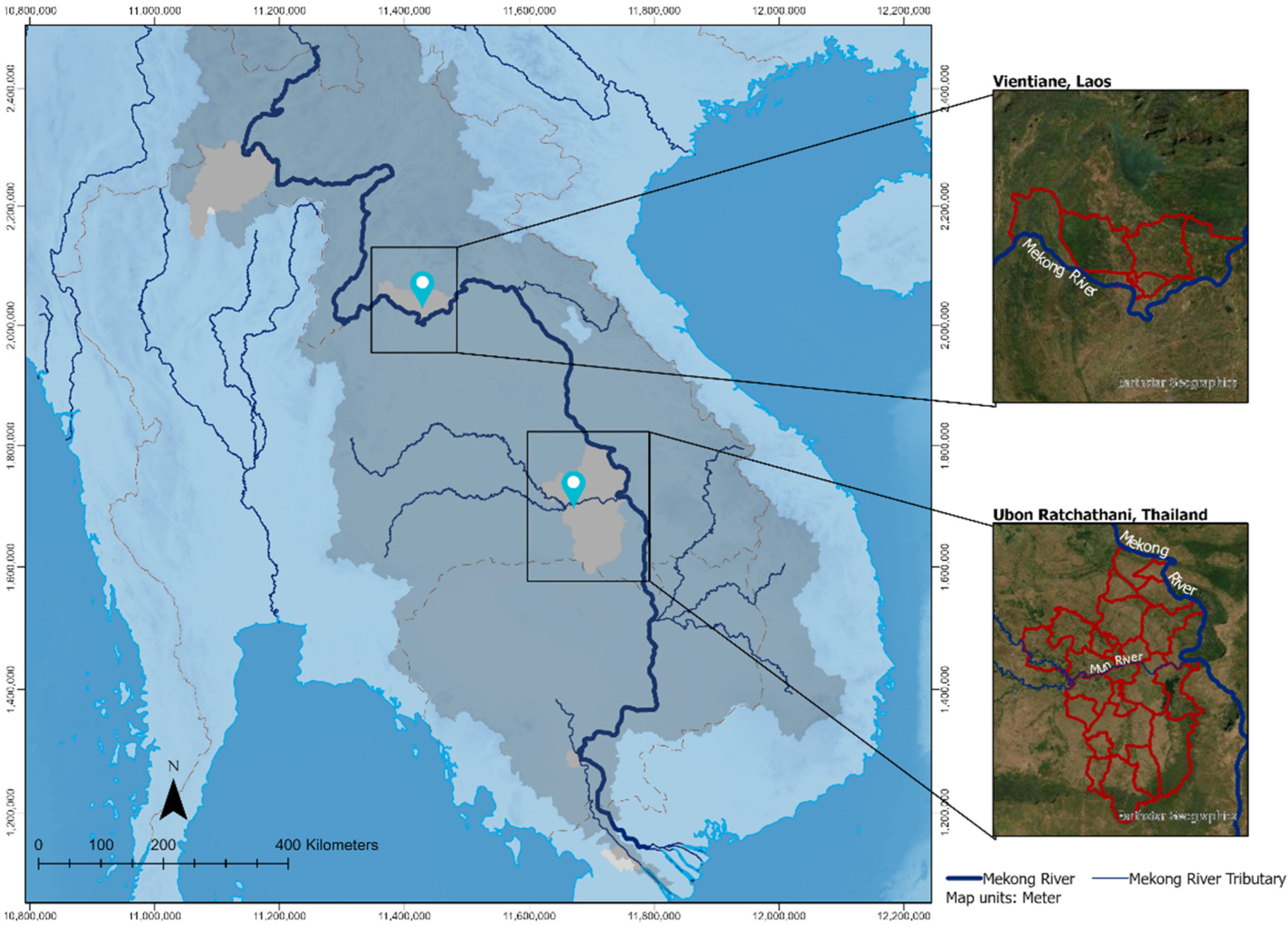
2.1. Study Area

The study site comprises the lower Mekong basin, an area home to nearly 65 million individuals dependent on the Mekong River sources [11]. Two cities located at intersections of the Mekong River and the Mun River, two important rivers in Southeast Asia, were investigated: Ubon Ratchathani, Thailand and Vientiane, Laos, as shown in Figure 1 below. The two cities feature differing topography and waste management practices which were taken into account. Our approach overlays plastic leakage distribution with the existing city-level waste management and regulation.

A macroplastic survey was conducted with assistance from local partners from the Ubon Ratchathani University in Ubon Ratchathani and the National University of Laos in Vientiane. The macroplastic survey involved visual interpretation of plastic material found in the environment using a mobile application. The survey took place during two seasons (wet and dry seasons) and focused on three types of areas where litter commonly occurs near or along the river: littering spots, uncontrolled dumps, and artificial barriers.

Ubon Ratchathani, a provincial in Thailand, creates 838.6 tons of solid waste daily, which is collected and disposed of at 28 dumpsites, 2 sanitary landfills, and 10 controlled dumpsites [12]. Most plastic waste disposal includes plastic bags, beverage bottles, and food wrappers. Ubon Ratchathani is responsible for 88.03% of accumulated plastic waste in the dry season (May–June 2021). Plastic waste profoundly affects the conditions of tourism and community residences, which is also prone to leakage in the weirs alongside the river.

Vientiane is the national capital of Laos PDR and generates approximately 760 tons of solid waste per day. The waste is managed in landfills [13], of which plastic waste accounts for 11.02% of solid waste in Vientiane [14]. Although waste collection service has doubled in the last ten years, some waste management facilities are poorly managed, leading to the leakages in the Mekong River.

2.2. Methodology

Plastic leakage was monitored according to the following designations: plastic leakage density, plastic leakage source hotspots, and leakage pathway accumulation. “Plastic leakage density” refers to an estimated quantity of plastic leakage in an area. However, the quantity was uncountable because the input parameters were normalized with a standard range from “0” to “1” for the fuzzy model concept. Areas were classified as either “0” for very low plastic leakage occurrence or “1” for very high plastic leakage occurrence. “Plastic leakage source hotspots” are the results of overlay analysis for the plastic leakage density map, the morphometric drainage map, and the distance to the nearest main river. Results ranged from very low (“0”) to very high (“1”). For example, areas featuring high or very high plastic leakage density along with high or very high drainage morphometric value (high value of drainage density, stream length, slope, etc.) would indicate a condition that contributes plastic to rivers. The final result of analysis was restricted to the subdistrict level as this was the finest-level data available. Furthermore, “leakage pathway accumulation” refers to scenarios that introduce plastic leakage inputs to waterways, such as a river, tributary, and canals.

To map and identify plastic leakage source hotspots and their pathways in the LMRB, the methodology was developed in three major phases (Figure 2): (1) data acquisition, (2) data analysis, and (3) plastic leakage source hotspots mapping. Moreover, an additional phase, (4) scenario development, was added to improve pathway accumulation in the waterway through scenario development. Data collection benefitted from the addition of ancillary data, mobile-app utilization, and macroplastic survey. Data analysis sought to determine indicators for plastic waste leakage through instances of plastic waste occurrence. Subsequently, plastic leakage source hotspot mapping was carried out using a combination of fuzzy overlay analysis along with hydrological analysis. Hydrological analysis led to development of a scenario to improve understanding of how plastic waste material is transported in the waterway at the sub-basin level.

2.2.1. Data Acquisition

Invariably, leakage of plastic litter into the marine environment is significantly triggered by anthropogenic activities that include: (i) general (intentional and unintentional) littering; and (ii) mismanaged or unmanaged plastic waste management systems that encompass phases such as production, use, collection, handling, storage, treatment, and disposal. Leaked plastic from the various aspects of the value chain may be washed away by surface runoff or blown by the wind into water environments via storm drains, canals, and rivers. Characteristically, artificial and other topographic barriers often create accumulation points for leaked plastic litter in rivers and canals before eventually being released into the ocean.

Understanding plastic leakage source hotspots are essential to assess the quantities of macro- and micro-plastics entering the ocean. This knowledge is required to indicate regional or local hotspots of occurrence and to determine the options for developing preventative measures. Therefore, a suite of indicators that presents a high potential correlation with plastic leakage was collected, including demographic information; topographic information; land use information; infrastructure; and satellite-based information. In addition, waste management information is also an essential indicator of reducing plastic waste entering the river and marine environment. Thus, it was collected and incorporated into the model to produce a plastic leakage source hotspots map. The leakage source hotspot map was created by overlaying the above indicators with the sub-basin morphometric analysis result. Moreover, the primary data (littering spots and uncontrolled dumpsites) collected using a mobile application have also been added as indicators. As the result of data acquisition, all the input indicators for the analysis are shown in

Table 1. Selected indicators for plastic leakage source hotspots mapping.

Indicators *		Study Sites		Data Type	Data Source
		Ubon Ratchathani	Vientiane
Static, Increase	Population Density	✓	✓	Raster	GIC-AIT WorldPop [15] Vientiane Capital Statistics Center [16]
	POIs Location	✓	✓	Point	Local Partners OSM [17]
	Land Use Information	✓	✓	Polygon	Local Partners
	Factory Location	✓	✓	Point	Local Partners
	Nighttime Image	✓	✓	Raster	USGS—VIIRS [18]
	Resident Types		✓	Raster	Local Partners
	Road	✓	✓	Line	Local Partners
	Slope	✓	✓	Raster	USGS—SRTM [19]
	Waste Generation	✓	✓	Polygon	Local Partners
	Open Dumpsite Location	✓		Point	PCD [12]
Static, Decrease	Waste Collection Coverage		✓	Line	VCOM [13]
	Waste Collection Route		✓	Line	VCOM [13]
	Waste Collection Service		✓	Point	VCOM [13]
Dynamic, Increase	Littering Spots	✓	✓	Point	Primary Data Collection by Local Partners

* See the complete list of indicators in Appendix A.

.

According to the Guidelines for the Monitoring and Assessment of Plastic Litter in the ocean [20], all indicators for plastic leakage mapping were divided into three categories: static, dynamic, and natural. In addition, each leading indicator was also divided into two types according to the impact of the plastic leakage: increase and decrease. Increase indicates higher waste leakage potential, while decrease refers to some activity or condition that could reduce plastic waste leakage, such as waste collection service.

To verify the plastic leakage density map, the city-scale plastic litter heatmap for Ubon Ratchathani generated by the pLitter platform was used to assess the accuracy of the overlay map. The pLitter platform is a standardized, deep learning-friendly dataset and pre-trained model used to detect plastic litter in streets, roadsides, and other outdoor locations [21]. The predicted result is used to produce the plastic litter heatmap for Ubon Ratchathani.

2.2.2. Fuzzy Overlay Analysis

Fuzzification is a comprehensive method to normalize multi-variable data parameters. As it is utilized to improve the function of multi-criteria spatial modelling, fuzzy overlay uses weighted parameters [22] to summarize the multi-variate data analysis, such as the plastic waste leakage issue [23]. Fuzzy overlay analysis in a GIS environment consists of three steps: (i) fuzzification of input variables by conversion into raster; (ii) assignment of fuzzy membership functions; and (iii) final fuzzy overlay and defuzzification to obtain the final output map.

• Fuzzification of Input Indicators

Datasets obtained for the selected indicators in Table 1 consisted of either point, line, or polygon vectors which were converted into raster values in each cell (fuzzification of input indicators) to run the fuzzy overlay analysis in the GIS. The datasets in point form were converted into raster using a kernel density to develop density information in spatial distribution. In GIS, kernel density computes the density of the point features in the neighborhood around them. In theory, a smooth curved surface is fit over each of the points, where the value is given to the highest point, which then decreases when it goes further up to 0, building up a circular neighborhood [24]. To address the data within locations and required distance or length, Euclidean distance was calculated for the indicators in the line form, which gives the center of the source of the cell to the mid-point of each neighboring cell. This shortest distance is the one that was allocated to the cell location on the output raster [25]. The Features to Raster tool converts vector features to a raster dataset for the indicators in the polygon form and already has an area state. This tool uses the cell center to decide the value of a raster cell. The input field type determines the type of output raster (for example, if the field is an integer, the output raster will be an integer; if it is a floating point, the output will be the floating point). The output cell size can be defined by a numeric value or obtained from an existing raster dataset. Rasterization methods for each vector type is illustrated in Figure 3.

• Assignment of Membership Functions

Based on the favorability of macroplastic leakage under each input indicator’s influence, the following membership functions were selected for this research: Linear, Large, Small, MS Large, and MS Small. Each of the functions has been identified to improve the proportional or inversely proportional relations. The Large and MS Large functions were used for the group increase of macroplastic, indicating that the higher the number of sources, the higher the outflow of macroplastic in the region. As for the road networks in the group of the increased macroplastic group, the Small function was used, which showed that the shorter the distance from these sources, the higher the leakage. The decreased macroplastic group followed similar logic, with input indicators assigned the Small and MS Small functions [26].

Among the static indicator group, the Small function was used for the slope indicator. Areas with low elevations favor higher human habitation, consequently raising the number of macroplastic sources. For the remaining variable in the static group, population, the linear function was applied, which meant that the outflow of macroplastic increases directly with the increase in the indicator’s value. It should be noted that resident type data was acquired from the classification of nighttime light raster data. Three classes were assigned to resident type: commercial area, urban residential area, and slum residential area. Slum residential area refers to the areas that contribute most to environmental plastic leakage. These raster data were reclassified on a scale of 1 to 3 based on the favorability of macroplastic leakage from the type of resident using the Reclassify tool in ArcGIS. Following reclassification, the Small membership function was applied.

• Fuzzy Overlay and Defuzzification

Fuzzy overlay was implemented after applying a membership function to each dataset. The available overlay functions in GIS are: AND, OR, PRODUCT, SUM, and GAMMA. Among all the overlay functions, “AND” was primarily used because it gives the membership the least common denominator, which considers all the indicators as the impact to the vulnerable condition (

Table 2. Functions used for raster conversion and membership for the indicators.

Data 1	Conversion into Raster	Spatial Resolution (Meter)	Membership Function	Remarks	Input Value		Output Value
					Min	Max	Min	Max
Population Density	Raster	30	Linear	As the population increases, the macroplastics leakage from the area also increases due to increase in use of plastics.	0	Max	0	1
Factory location	Kernel Density	30	MS Large	Larger the number of factories in an area, higher the leakage of macroplastics.	0	Max	0	1
Resident type	Raster	30	Small	Smaller the value of scale, larger the macroplastics leakage.	0	Max	0	1
Road	Euclidean Distance	30	Small	Smaller the distance from the road networks, higher the leakage of macroplastics.	0	Max	0	1
Slope	Raster	30	Small	Smaller slope favors human inhabitation, which increases macroplastic leakage.	0	20	0	1
Waste generation	Kernel Density	30	MS Large	Larger the amount of waste generated in an area, higher the leakage of macroplastics.	0	Max	0	1
Open dumpsite location	Kernel Density	30	Large	Larger the number of open dumpsites in an area, higher the leakage of macroplastics.	0	Max	0	1
Waste collection coverage	Kernel Density	30	Small	Smaller the number of waste collection coverage in an area, higher the leakage of macroplastics.	0	Max	0	1
Waste collection route	Euclidean Distance	30	Small	Smaller the number of waste collection routes in an area, higher the leakage of macroplastics.	0	Max	0	1
Waste collection services	Kernel Density	30	MS Small	Smaller the number of waste collection services in an area, higher the leakage of macroplastics.	0	Max	0	1
Littering spot	Kernel Density	30	Large	Larger the number of littering spots in an area, the larger the leakage of macroplastics.	0	Max	0	1
POIs 2	Kernel Density	30	Large	Larger the number of POIs, the higher the leakage of macroplastics.	0	Max	0	1

¹Appendix A: Definition of the input indicator. ² Point of Interest (POI) locations include hotels, restaurants, facilities other public facilities.

). This allows us to see the effect of each indicator on the leakage of macroplastics from the region.

The “PRODUCT” function was used exclusively for uncontrolled dumpsites and littering spots. This function identifies the highest membership values of the input, which can eliminate the higher potential of leakage occurrence. Other functions such as “OR”, “SUM”, and “GAMMA” were not applicable in this case as these overlay functions showed the combined effect of all the indicators. Multiple overlays were run for each indicator group and then combined to obtain a final output map.

The final overlay map displayed output values between 0 and 1, where 1 represented full membership (leakage) and 0 represented non-membership (non-leakage). These values had to be defuzzied to quantify the values to be represented on a map. Hence, the values were reclassified in GIS into five classes to indicate macroplastic leakage potential: low, very low, medium, high, and very high. The values near 0 were classified as low, and those near 1 were classified as very high.

2.2.3. Accuracy Assessment

In a statistical context, accuracy indicates the degree of correctness of a classified map, consisting of bias and precision. The accuracy check compares the plastic leakage density map with plastic littering hotspot locations (confusion matrix,

Table 3. General confusion matrix for a plastic leakage density map. The confusion matrix shows the number of correctly classified points (True, green diagonal) and wrongly classified (False, red diagonal).

Ground Truth	Classification Result
	Leakage Hotspot (A)	Non-Leakage Hotspot (B)
Leakage Hotspot (A)	True (a)	False (b)
Non-Leakage Hotspot (B)	False (c)	True (d)

). A total of 432 samples were used, including 164 sample locations of littering spots and 268 sample locations of non-littering spots. It is recommended to obtain ground truth data near the time of data acquisition, especially before any environmental change.

In addition to the confusion matrix, user’s, producer’s, and overall accuracies (OA) and kappa statistics were produced (Table 3).

Overall accuracy

The OA evaluates the overall effectiveness of the algorithm. It is calculated as the total number of correctly-classified points (green diagonal in Table 3) divided by the total number of validation points:

$$OA=\frac{No. of correct points}{Total number of points}$$

User’s accuracy

The user’s accuracy, also called precision, refers to the fraction of correctly classified points regarding all points categorized as this class in the classification results. The user’s accuracy evaluates the fraction of correctly classified leakage hotspot points compared to all points that were classified (classification result) as leakage hotspots (true and false). Therefore, precision considers the number of non-leakage hotspot points that were misclassified as leakage hotspots.

For the leakage hotspot class:

$$User acc\left(A\right)=\frac{a}{a+b}$$

For the non-leakage hotspot class:

$$User acc\left(B\right)=\frac{d}{c+d}$$

Producer’s accuracy

The producer’s accuracy, also called recall, is defined as the correctly classified points of a class (e.g., A) related to all points of the considered ground truth class (Ground Truth). Recall looks at the number of points classified as A and compares them to the reference ground-truth dataset for class A. Recall considers the number of crop points that were misclassified as non-leakage hotspots.

For the leakage hotspot class:

$$Prod. acc\left(A\right)=\frac{a}{a+c}$$

For the non-leakage hotspot class:

$$Prod. acc\left(B\right)=\frac{d}{b+d}$$

F-score

The F-score is a valuable measure of error as it combines both the user’s accuracy and the producer’s accuracy of a class. It can be interpreted as the harmonic mean of both error measures, with a maximum value of 1 and a minimum score of 0 [1].

For the F-score of leakage hotspots:

$$Fscore\left(A\right)=2\times \frac{User acc\left(A\right)\times Prod. acc\left(A\right)}{User acc\left(A\right)+Prod. acc\left(A\right)}$$

For the F-score of the non-leakage hotspots:

$$Fscore\left(B\right)=2\times \frac{User acc\left(B\right)\times Prod. acc\left(B\right)}{User acc\left(B\right)+Prod. acc\left(B\right)}$$

2.2.4. Morphometric Analysis and Leakage Pathway Accumulation Scenario Development

• Morphometric Analysis

Morphometric analysis was used to deliver quantitative measurement and mathematical analysis for landforms [27]. This method uses DEM extraction for delivering the morphometric parameters which define the estimated landform. This method of analysis, also referred to as the static and semi-dynamic analysis for characterizing the hydrological responses between topographical features within the sub-basin, led to the watershed implication; stream, including river and its tributaries, led to canal networks. To comply with the method, 22 parameters were developed to differentiate features from a Shuttle Radar Topography Mission (SRTM) 30 m DEM [19]. We also developed the supporting sub-category from the shape form of sub-basin characteristics and the development of each drainage network using weighed on scale and topography measurement. This approach is utilized by previous studies related to flash floods and hydrological response towards peak runoff [8,9,27,28,29], where flash flood events were used to understand the probability of water flow and sub-basin level material shifts [30]. To deliver the morphometric analysis related to the hydrological characteristics, several morphometric parameters were grouped into the four aforementioned classes: scale, topographic, shape, and drainage network (Appendix B). Previously, the identification was initiated by identifying the watershed area, shown in Figure 4 below.

Morphometric analysis can be used to describe the hydrology characteristics of sub-basins, which over time establish their own qualities that can differ from the larger basin they originate from. Characteristics such as flow and material transport are used to realize the plastic waste leakage source hotspots where land-based interface with waterbodies. A 30 m resolution DEM was generated to identify streams and the sub-basin (watershed), followed by zonal processing for 22 parameters (Appendix B). The zonal process involved the calculation of each parameter by zones, which are delineated areas of the watershed. Subsequently, all parameters were calculated and combined for weighting values to produce the hydrological characteristics.

• Sub-basin Analysis for Plastic Leakage Source Hotspots

According to [31], areas with high drainage density with both high runoff and high probability of flooding within the hydrological characteristic, yet improved the material shifting along with blockage in the waterway. In addition, there is a higher potential for flooding when increased flow brings more plastic to the channel [32]. Communities that have high to very high potential for plastic leakage density and high or very high drainage density will introduce plastic pollution into waterways. Based on this concept, the possible plastic leakage density map and drainage morphometry map were used to identify plastic pathways. Figure 5 below shows a conceptual diagram of identifying communities that contribute to riverine plastic pollution.

• Leakage Pathway Accumulation Scenario Development

After the characteristics for all obtaining watersheds in each study area were identified, the result of drainage morphometry was utilized to improve the leakage pathway accumulation. The framework for the plastic leakage pathway accumulation is shown in Figure 6.

The combination is applied in three steps: (1) identification of hydrological characteristics in the waterway; (2) calculation of weight based on the proximity of leakage source hotspot to the waterway; and (3) reclassification of the waterway using five classes (very low, low, medium, high, and very high). Proximity also regarded the distance between the plastic leakage source hotspot location and the delineated waterway, where the possibility was higher for hotspots located closer to the river.

Weight-based calculations were made after arriving at the results for hydrological characterization. Weights were assigned based on: proximity analysis, flooding record detection, and rainfall rate. Overall components were assembled to generate by the scoring system to define the higher occasions and prone to flash flood probability before the hydrological characteristics based on morphometric analysis. Therefore, the weight was overlaid and calculated based on the overlapped plastic waste source hotspot results.

Based on the leakage source hotspot map for land-based plastic waste, there were leakages occurring within the riverine pathway to the ocean. Hydrological characterization was used to realize hotspots at the river. Sequentially, leakage pathway accumulation is divided into 5-class assessed potential. Each regarded class is produced by calculating the result from the plastic leakage source hotspots and the hydrological characteristic in the sub-basin level.

3. Results

The macroplastics leakage density map was produced based on a fuzzy overlay of static and dynamic indicator groups to access region-level macroplastics pollution. Overlay of these major indicator groups provided insight for how macroplastics are leaked into waterways in the area. The output maps in this section show the macroplastics leakage density for a very low to very high range.

3.1. Plastic Leakage Source Hotspots Mapping

3.1.1. Plastic Leakage Density Map

Overlaid parameters include static and dynamic macroplastics which are based on indicators that define the waste sources in a particular region. The overlay map of the indicators in Figure 7 shows the intensity of two main groups of macroplastics leakage in Vientiane and Ubon Ratchathani.

The sub-districts with the highest macroplastics leakage density are in dark red color (very high potential of plastic leakage density which is potentially leaking into the environment), followed by red color (high potential), orange color (medium potential), yellow color (low potential), and transparent light-yellow color (very low potential). According to the input indicators under the static group (POIs, residential area, road network, industries, waste generation, and waste management) and dynamic group (human littering and uncontrolled dumpsites), the distribution concentrated prevalently in the center of the province/city and surrounding districts/sub-districts. Along with identifying leakage source hotspots which were derived from the result from the direct survey, plastic leakage is highly concentrated in the center, which is an urban area. Therefore, we expect great potential for leakage in the center as the urban area would likely have high intensity of human activity, causing more plastic waste leakage.

Although the concentrated area in the city and province is ranked in the high leakage category, it might be reduced with a proper waste management scheme. To address this, we reached out to the local municipality in Vientiane to gain information about the waste management plant. In collaboration with the municipality, a GPS Logger was used to track the routes of waste disposal trucks. The waste management route was used to gain insights into potential areas of environmental leakage.

This study included static and dynamic indicators based on the input indicator used in plastic leakage density identification. Static indicators performed more sensitive analysis because more indicators were conducted than with dynamic ones. This is implied in the study’s objective, where the plastic waste leakage source (especially the primary source) must be defined. Thus, the sources from the static indicators encompassed the control mechanism for reducing plastic leakage in terms of upstream approaches such as policy enforcement and development of a roadmap for reducing plastic waste generation in the first place.

As dynamic indicators can be managed with the efforts and approaches, the results of leakage source density have greater impact. There is still insufficient awareness for the impacts of littering on plastic leakage in dense urban centers where there is high intensity of human activity. In this case, a downstream approach such as a citizen science clean-up event might be the most applicable control mechanism to curb littering in urban areas.

3.1.2. Accuracy Assessment of Plastic Leakage Density Map in Ubon Ratchathani

Based on the fuzzy overlay analysis result in Ubon Ratchathani, the plastic leakage density map was classified into two classes: leakage hotspot and non-leakage hotspot. The leakage hotspot class is the result of merging three classes from the map: medium, high, and very high plastic leakage density. The non-leakage hotspot class is the combined result of low and very low plastic leakage density classes. From the plastic littering heatmap, a random sample of 432 points for leakage hotspots (164 points) and non-leakage hotspots (268 points) were extracted to validate the plastic leakage density map using a confusion matrix (

Table 4. The error matrix for the plastic leakage density map compared with plastic littering hotspots locations resulted from the pLitter.

Plastic Littering Hotspot Locations	Plastic Leakage Density Mapping Result
	Leakage Hotspot	Non-Leakage Hotspot
Leakage Hotspot	61	103
Non-Leakage Hotspot	149	119
Producer Accuracy	29.05%	53.60%
User Accuracy	37.20%	44.40%
F-score	0.33	0.49
Overall Accuracy	41.67%

).

The accuracy check of the classified map generated an overall accuracy of 41.67%, with an F-score of 0.33 (leakage hotspot) and 0.49 (non-leakage hotspot). Producer accuracy of leakage hotspot and non-leakage hotspot classes was 29.05% and 53.60%, while user accuracy of the two classes was 37.20% and 44.40%, respectively. The procedure accuracy (sensitivity) measure reflects the accuracy of prediction of leakage hotspot or non- leakage hotspot class. Furthermore, the accuracy of the plastic leakage density map demonstrates the user’s reliability. For example, the non-leakage hotspot was more reliable, with 44.40% user accuracy, than the leakage hotspot (37.20%).

3.1.3. Plastic Leakage Source Hotspots Map

The output map generated after running the fuzzy overlay with the indicator, including morphometric analysis results and plastic leakage density maps, are shown in Figure 8 and Figure 9. The map shows that the major pathways for macroplastic leakage are the high morphometric areas directly under the influence of facilities, infrastructure, and population. Larger morphometric areas next to the major contributors of static indicators are the ones that are causing the highest leakage of macroplastic.

As the capital city of Lao PDR with the Mekong River flowing between its border with Thailand, Vientiane implemented an advanced control mechanism to restrict its waste from entering the waterway. As seen in Figure 8, most of the hotspots in Vientiane are city pavement categorized as “very high”. One “high” hotspot is located along the shipment area (Figure 7B), which concerns higher leakage that is possibly generated in the commercial area. Similarly, Ubon Ratchathani’s result (Figure 8) has a high to very high source hotspot near the Mun River. Another high hotspot in Ubon Ratchathani is located at Si Mueang Mai, close to Huai Tung Lung River, which feeds into the Mun River (Figure 9C).

3.2. Leakage Pathway Accumulation

The hydrological characteristics improved the potential of flash flood occurrence regarding runoff. In the context of leakage, it allows us to define the probability higher classes located in the flood hazard area within proximity to higher leakage source hotspots. Figure 10 and Figure 11 show how the distribution for city-level leakage pathway accumulates along the river. Here, a base map helps to visualize the distribution of urban areas and their effect on leakage into nearby waterways along with the recorded floodplain to be considered.

According to the findings, the river accumulation type is divided into two general judgments: hotspots in the mainstream (Ubon Ratchathani) and tributaries from the mainstream (Vientiane). Based on the sparse in the hotspot, leakage pathway accumulation is concentrated in the urban areas of Ubon Ratchathani and Vientiane. All leakage pathway accumulation types are regarded as the result of the plastic waste leakage source hotspot.

Some factors are chronically affected by the plastic leakage accumulation in the waterway. Firstly, there are flood hazards. The hydrological characteristics refer to the peak runoff, and the prone to flood will be sensitively detected regarding the higher accumulation of plastic retained in the waterway. Regarding the 10-year period of flooding record history in Ubon Ratchatani (shown in the map Figure 11 with red transparent polygon), widespread and concentrated flooded area implies the different types of accumulation. Where the more concentrated area of flood-impacted to the “very high” categorized prone to leakage accumulation, this also proves that the condition of flood and plastic accumulation affect each other [33].

Another impact of the higher accumulation is the condition of the waste management services provided. Imploring from the regulation applied to dispose of the solid waste regarding plastic waste, disposal to the waterway could occur due to the overloaded capacity or improper management.

According to the waste management service, one of the stages that impacted the leakage events more is the collection system. Along with the same condition as the waste management services, the collection system implies the occurrence of the littering spots and uncontrolled dumpsites caused by uncollected waste. This condition is also conducted to identify land-based waste disposed into the waterway with a lack of collection [34]. We saw, in Vientiane, how the analysis impacted the recorded route using the GPS Logger, which led to a lower accumulation of leakage in the mainstream and “very low” categorized leakage in the rural areas.

Lastly, the riverbank environment impacts the amount of leakage. It is regarded from the riverbank area’s rejuvenation and revitalization, whether it has more pavement or vegetation. According to [6], city pavement causes more plastic input to the river. A similar case improved from the concentrated leakage pathway accumulation in the urban area, which also occurred in both study areas.

4. Discussion

This study used comparisons of primary data collection from littering spots to determine the degree of plastic leakage into waterways. With a mobile app designed to streamline macroplastic survey data collection, we compared our GIS-based modelling analysis with the primary data collection to calculate the density based on the recorded data acquisition in the particular locations. The density of littering spots to the nearest riverbank area aided in understanding potential leakage sources to the waterway. An index calculation was implemented between pathway accumulation and the littering spot density to provide a comparison in which higher accumulation impacted the higher index regarding littering spots.

As shown in Figure 12 above, the relationship between the littering spots and pathway accumulation is proportionally linear. According to the index calculation, the higher littering hotspot density occupies the higher accumulation index in the river. Leakage accumulation in Ubon Ratchathani represents a gradual correlation between littering spot density and pathway accumulation in the river. As seen in Figure 10, leakage in Ubon Ratchathani is varied, and most of the higher density of leakage sources implied high to very high accumulation. This also defined how the concentrated accumulation depends on the littering spots in the same configuration.

Unlike provincial Ubon Ratchathani in Thailand, Vientiane capital implored a more stagnant comparison. As more results are detected in very low to low accumulation, Vientiane still features a more concentrated accumulation in higher littering spots. However, accumulation categorized as “high” is concentrated on the higher leakage density index (4–8.5), implying the relative linear proportion with the field survey. Vientiane also detects more concentrated higher leakage in the higher density, leading to the probability of leakage in the urban area.

There is a correlation of the material accumulation in the waterway where both findings show higher accumulation in the urban area. This also implies the higher intensity of human activity, which leads to more littering spots, impacting the accumulation and abundance of plastic waste leakage. Some previous studies on riverine plastics were detected in urban areas with a high density of settlement [6,7,35,36]. However, this also indicated that a control mechanism at the riverbank for the littering spots is the direct solution.

For further direct solutions, the result of plastic leakage source hotspots was compiled with the amount of plastic leakage detected in the waterway. Therefore, an improvement in measuring the plastic waste discharge to the river should comprehend the control mechanism. In addition, real-time monitoring integrated with closed-circuit monitoring assisted the mitigation system for plastic leakage in the waterway.

5. Conclusions

The overall efforts in this study demonstrate the effectiveness of the proposed method for predicting plastic leakage density and its sources using multi-source geospatial data with a fuzzy overlay approach. Here, the methodology is compatible with the mitigation system for preventing plastic leakage in the provincial and capital areas. This approach can be more cost-effective and practical once tailored to meet each case’s use. The application of fuzzy overlay methodology and overlay analysis together can be used as a rapid assessment tool when the model is updated to use only secondary open data available online. To support this approach, fast field surveys and assessments should be conducted in priority areas.

Moreover, the increased urbanization and population growth rate are responsible for an unaccountable amount of plastic pollution [37]. Thus, if we have limited to no action, the plastic pollution crisis will occur in the LMRB in the future. Therefore, this approach addresses the initial downstream approach to combat the exiting plastic waste in the environment.

References

1. ASEAN. Regional Action Plan for Combating Marine Debris in the ASEAN Member States. Jakarta, ASEAN Secretariat. Available online: https://asean.org/wp-content/uploads/2021/05/FINAL_210524-ASEAN-Regional-Action-Plan_Ready-to-Publish_v2.pdf (accessed on 8 November 2021).
2. Peng, Y.; Wu, P.; Schartup, A.T.; Zhang, Y. Plastic waste release caused by COVID-19 and its fate in the global ocean. Proc. Natl. Acad. Sci. USA 2021, 118, e2111530118. [Google Scholar] [CrossRef] [PubMed]
3. Borrelle, S.B.; Ringma, J.; Lavender Law, K.; Monnahan, C.C.; Lebreton, L.; McGivern, A.; Murphy, E.; Jambeck, J.; Leonard, G.H.; Hilleary, M.A.; et al. Predicted growth in plastic waste exceeds efforts to mitigate plastic pollution. Science 2020, 369, 1515–1518. [Google Scholar] [CrossRef] [PubMed]
4. Harris, P.T.; Westerveld, L.; Nyberg, B.; Maes, T.; Macmillan-Lawler, M.; Appelquist, L.R. Exposure of coastal environments to river-sourced plastic pollution. Sci. Total Environ. 2021, 769, 145222. [Google Scholar] [CrossRef] [PubMed]
5. Lebreton, L.C.M.; van der Zwet, J.; Damsteeg, J.W.; Slat, B.; Andrady, A.; Reisser, J. River plastic emissions to the world’s oceans. Nat. Commun. 2017, 8, 15611. [Google Scholar] [CrossRef] [PubMed]
6. Meijer, L.J.J.; van Emmerik, T.; van der Ent, R.; Schmidt, C.; Lebreton, L. More than 1000 rivers account for 80% of global riverine plastic emissions into the ocean. Sci. Adv. 2021, 7, eaaz5803. [Google Scholar] [CrossRef] [PubMed]
7. Sakti, A.D.; Rinasti, A.N.; Agustina, E.; Diastomo, H.; Muhammad, F.; Anna, Z.; Wikantika, K. Multi-scenario model of plastic waste accumulation potential in indonesia using integrated remote sensing, statistic and socio-demographic data. ISPRS Int. J. Geoinf. 2021, 10, 481. [Google Scholar] [CrossRef]
8. Rekha, V.B.; George, A.V.; Rita, M. Morphometric analysis and micro-watershed prioritization of peruvanthanam sub-watershed, the Manimala river basin, Kerala, South India. Environ. Res. Eng. Manag. 2011, 57, 6–14. [Google Scholar]
9. Harsha, J.; Ravikumar, A.S.; Shivakumar, B.L. Evaluation of morphometric parameters and hypsometric curve of Arkavathy river basin using RS and GIS techniques. Appl. Water Sci. 2020, 10, 86. [Google Scholar] [CrossRef] [Green Version]
10. Pande, C.B.; Moharir, K. GIS-based quantitative morphometric analysis and its consequences: A case study from Shanur River Basin, Maharashtra India. Appl. Water Sci. 2017, 7, 861–871. [Google Scholar] [CrossRef] [Green Version]
11. Mekong River Commission (MRC). People of Mekong Basin. Available online: https://www.mrcmekong.org/about/mekong-basin/people/ (accessed on 19 January 2022).
12. Thailand Pollution Control Department. Information on the Situation of Solid Waste in Ubon Ratchathani Province. Available online: https://thaimsw.pcd.go.th/report_province.php?year=2563&province=23 (accessed on 15 March 2022).
13. VCOM. Sustainable Solid Waste Management Strategy and Action Plan for Vientiane 2020–2030; VCOM: Vientiane, Laos, 2021. [Google Scholar]
14. EEP. Feasibility Study of the SWM Project in Vientiane. Vientiane: Energy and Environment Partnership-Mekong; The Energy and Environment Partnership (EEP) Mekong: Vientiane, Laos, 2015. [Google Scholar]
15. WorldPop. Population Density. Available online: https://www.worldpop.org/project/categories?id=18 (accessed on 7 March 2022).
16. Vientiane Capital Statistics Center. Population. Available online: https://psc-vt.lsb.gov.la/ (accessed on 7 March 2022).
17. Open Street Map. Available online: https://www.openstreetmap.org/#map=6/13.149/101.493 (accessed on 8 November 2021).
18. NASA USGS. Visible Infrared Imaging Radiometer Suite (VIIRS) Overview. Available online: https://lpdaac.usgs.gov/data/get-started-data/collection-overview/missions/s-npp-nasa-viirs-overview/ (accessed on 8 November 2021).
19. NASA USGS Earth Resources Observation and Science (EROS) Center. USGS EROS Archive—Digital Elevation—Shuttle Radar Topography Mission (SRTM) Non-Void Filled. Available online: https://www.usgs.gov/centers/eros/science/usgs-eros-archive-digital-elevation-shuttle-radar-topography-mission-srtm-non (accessed on 15 August 2021).
20. GESAMP (Joint Group of Experts on the Scientific Aspects of Marine Environmental Protection). Guidelines for the Monitoring and Assessment of Plastic Litter in the Ocean. IMO, FAO, UNESCO-IOC, UNIDO, WMO, IAEA, UN, UN Environment, UNDP, ISA. GESAMP Report and Studies No. 99. Available online: http://www.gesamp.org/publications/guidelines-for-the-monitoring-and-assessment-of-plastic-litter-in-the-ocean (accessed on 24 January 2022).
21. Geoinformatics Center, Asian Institute of Technology. pLitter. Available online: https://plitter.org/ (accessed on 9 March 2022).
22. Baidya, P.; Chutia, D.; Sudhakar, S.; Goswami, C.; Goswami, J.; Saikhom, V.; Singh, P.S.; Sarma, K.K.; Baidya, P.; Chutia, D.; et al. Effectiveness of fuzzy overlay function for multi-criteria spatial modeling—A case study on preparation of land resources map for mawsynram block of East Khasi hills district of Meghalaya, India. Int. J. Geogr. Inf. Sci. 2014, 6, 605–612. [Google Scholar] [CrossRef] [Green Version]
23. Chukwuma, E.C.; Shariff, A.R.B.M.; Hasfalina, C.M.; Mohamed, A.A.; Abdullah, L.C. GIS-based analysis of plastic waste leakage in parts of Selangor state of Malaysia. In Proceedings of the ASABE Annual International Meeting, Boston, MA, USA, 7–10 July 2019; pp. 1–18. [Google Scholar]
24. Silverman, B.W. Density Estimation for Statistics and Data Analysis; Routledge: New York, NY, USA, 2018. [Google Scholar]
25. ESRI. Euclidean Distance [Spatial Analyst]—ArcMap Documentation. Available online: https://desktop.arcgis.com/en/arcmap/latest/tools/spatial-analyst-toolbox/euclidean-distance.htm (accessed on 15 August 2021).
26. ESRI. How Fuzzy Membership Works—ArcGIS for Desktop. Available online: https://desktop.arcgis.com/en/arcmap/latest/tools/spatial-analyst-toolbox/how-fuzzy-membership-works.htm (accessed on 15 August 2021).
27. Adnan, M.S.G.; Dewan, A.; Zannat, K.E.; Abdullah, A.Y.M. The use of watershed geomorphic data in flash flood susceptibility zoning: A case study of the Karnaphuli and Sangu river basins of Bangladesh. Nat. Hazards 2019, 99, 425–448. [Google Scholar] [CrossRef]
28. Abdel-Fattah, M.; Saber, M.; Kantoush, S.A.; Khalil, M.F.; Sumi, T.; Sefelnasr, A.M. A hydrological and geomorphometric approach to understanding the generation of wadi flash floods. Water 2017, 9, 553. [Google Scholar] [CrossRef] [Green Version]
29. Asfaw, D.; Workineh, G. Quantitative analysis of morphometry on Ribb and Gumara watersheds: Implications for soil and water conservation. Int. Soil Water Conserv. Res. 2019, 7, 150–157. [Google Scholar] [CrossRef]
30. Destro, E.; Amponsah, W.; Nikolopoulos, E.I.; Marchi, L.; Marra, F.; Zoccatelli, D.; Borga, M. Coupled prediction of flash flood response and debris flow occurrence: Application on an alpine extreme flood event. J. Hydrol. 2018, 558, 225–237. [Google Scholar] [CrossRef]
31. Sreedevi, P.D.; Sreekanth, P.D.; Khan, H.H.; Ahmed, S. Drainage morphometry and its influence on hydrology in an semi-arid region: Using SRTM data and GIS. Environ. Earth Sci. 2013, 70, 839–848. [Google Scholar] [CrossRef]
32. Tjia, J.A.L. Assessing the impact of plastic waste accumulation on nood events with citizen observations A case study in Kumasi, Ghana. Available online: http://repository.tudelft.nl/ (accessed on 19 May 2022).
33. Honingh, D.; van Emmerik, T.; Uijttewaal, W.; Kardhana, H.; Hoes, O.; van de Giesen, N. Urban river water level increase through plastic waste accumulation at a rack structure. Front. Earth Sci. 2020, 8, 28. [Google Scholar] [CrossRef]
34. Verster, C.; Bouwman, H. Land-based sources and pathways of marine plastics in a South African context. S. Afr. J. Sci. 2020, 116, 1–9. [Google Scholar] [CrossRef]
35. Cordova, M.R.; Nurhati, I.S. Major sources and monthly variations in the release of land-derived marine debris from the Greater Jakarta area, Indonesia. Sci. Rep. 2019, 9, 18730. [Google Scholar] [CrossRef] [PubMed]
36. van Emmerik, T.; Loozen, M.; van Oeveren, K.; Buschman, F.; Prinsen, G. Riverine plastic emission from Jakarta into the ocean. Environ. Res. Lett. 2019, 14, 084033. [Google Scholar] [CrossRef] [Green Version]
37. Hoornweg, D.; Bhada-Tata, P. What a Waste—A Global Review of Solid Waste Management (Rep. No. 15). March 2012. Available online: https://siteresources.worldbank.org/INTURBANDEVELOPMENT/Resources/3363871334852610766/What_a_Waste2012_Final.pdf (accessed on 24 January 2022).
Figure 1. Location of the study area along the lower Mekong basin.
Sustainability 14 07879 g001
Figure 2. Flowchart of methodology to map plastic source hotspots and their pathway in the lower Mekong basin.
Sustainability 14 07879 g002
Figure 3. Rasterization methods: (A) Kernel Density, (B) Euclidean Distance, and (C) Features to Raster.
Sustainability 14 07879 g003
Figure 4. Morphometric analysis methodology.
Sustainability 14 07879 g004
Figure 5. Defining leakage source hotspot using morphometric analysis in sub-basin from fuzzy overlay results.
Sustainability 14 07879 g005
Figure 6. Framework to the leakage pathway accumulation.
Sustainability 14 07879 g006
Figure 7. Identified plastic density hotspots based on static and dynamic indicator groups: (A) Ubon Ratchathani province and (B) Vientiane capital.
Sustainability 14 07879 g007
Figure 8. Plastic leakage source hotspots in Vientiane. Dark-red color indicates very high plastic leakage sources, and yellow shows very low plastic leakage sources in the city.
Sustainability 14 07879 g008
Figure 9. Plastic leakage source hotspot in Ubon Ratchathani.
Sustainability 14 07879 g009
Figure 10. Plastic leakage pathway accumulation in Vientiane capital, Laos.
Sustainability 14 07879 g010
Figure 11. Leakage pathway accumulation in Ubon Ratchathani province, Thailand.
Sustainability 14 07879 g011
Figure 12. Comparisons of leakage pathway accumulation with surveyed littering spots in (a) Ubon Ratchathani and (b) Vientiane capital.
Sustainability 14 07879 g012