
Experimental and Numerical Analysis on Effect of Passive Cooling Methods on an Indoor Thermal Environment Having Floor-Level Windows


Abstract
:1. Introduction
2. Methods
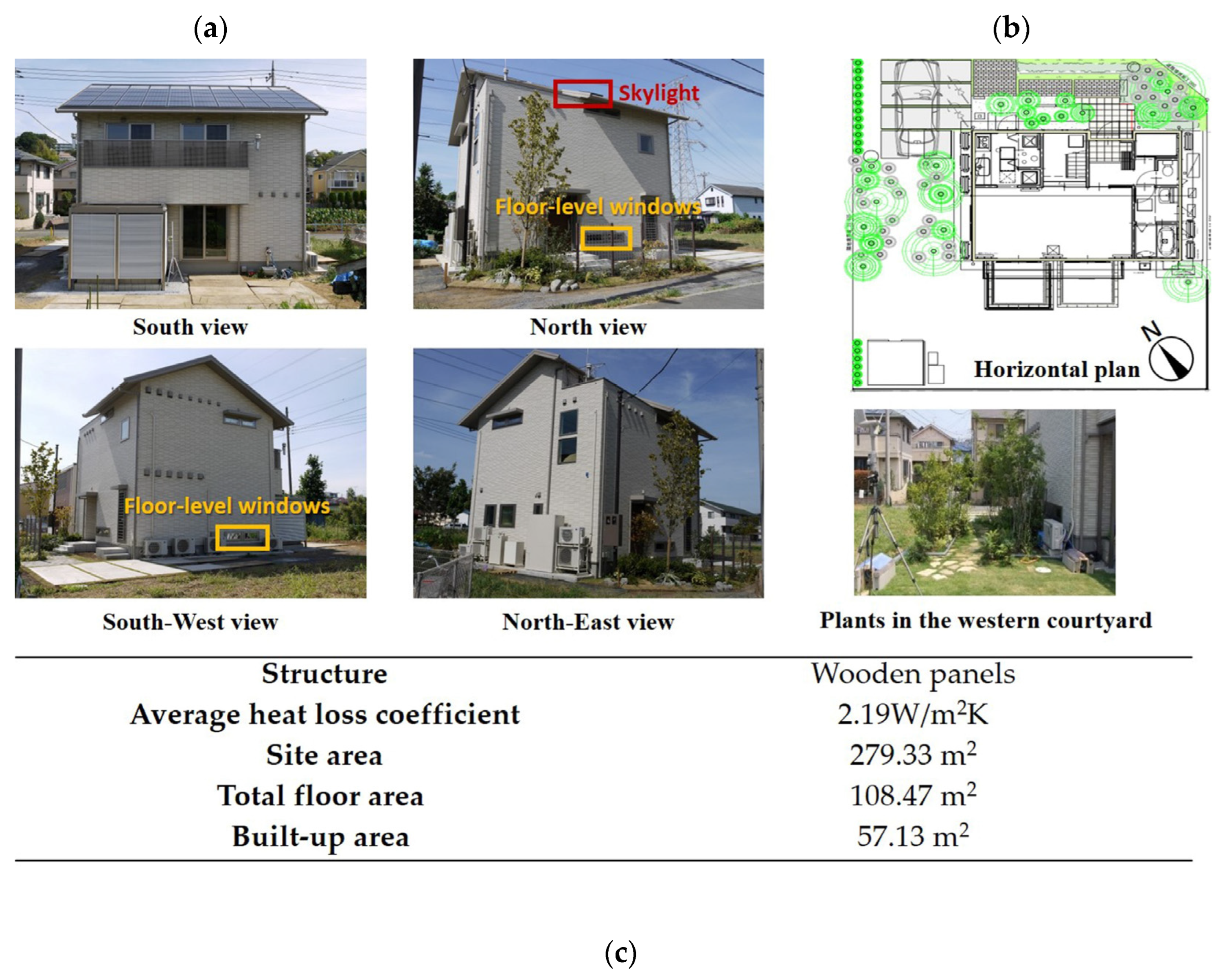
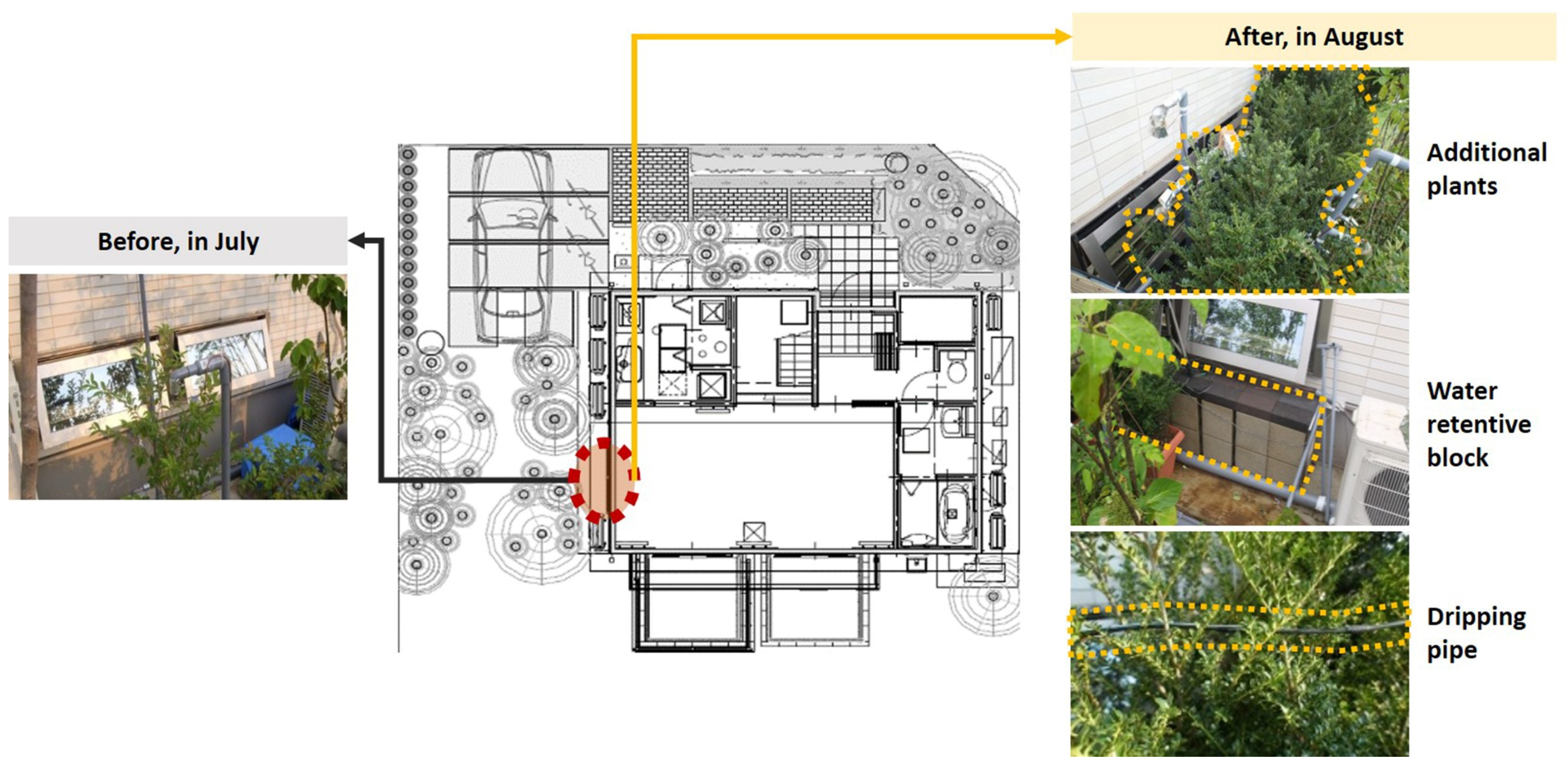
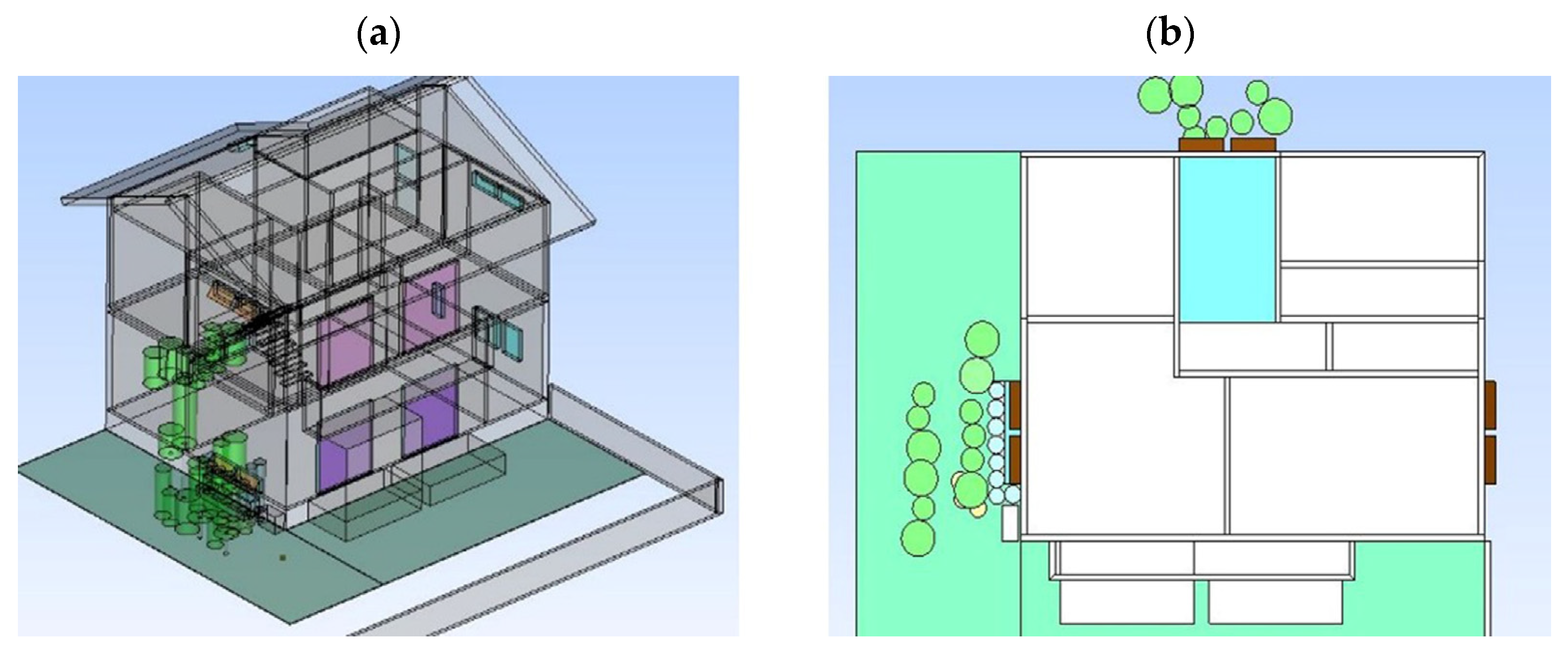
2.1. Study House and Its Passive Cooling Design
2.2. Experiment
2.2.1. Experiment Condition
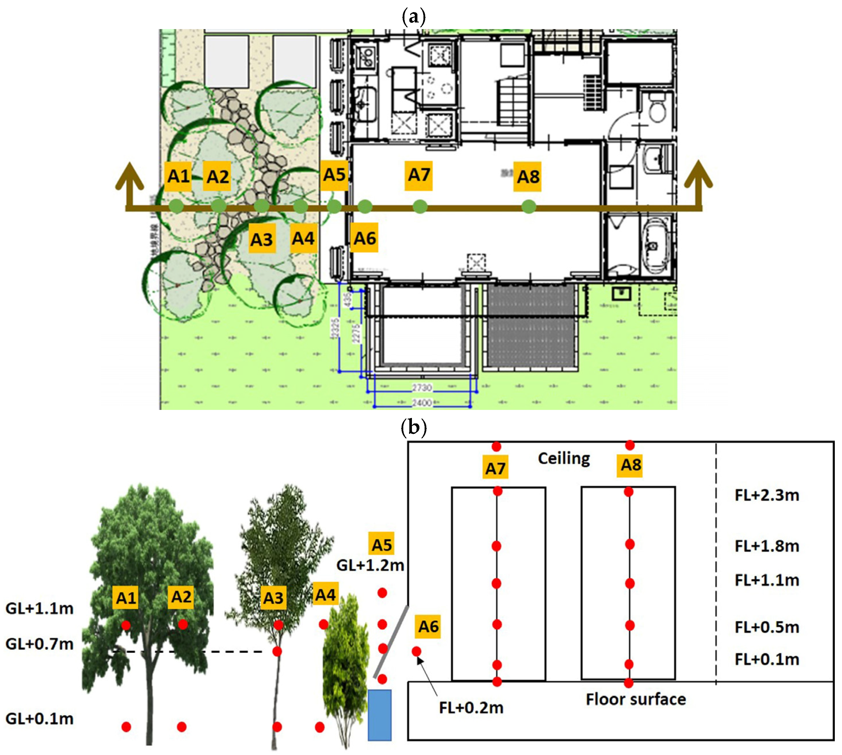
2.2.2. Measurement Points and Instruments
2.3. Computational Fluid Dynamics (CFD) Simulation
2.3.1. Simulation Method
2.3.2. Sensitivity Analysis on the Floor-Level Window Design
2.3.3. Investigation on Cooling Effect by Passive Cooling Design
2.4. Calculation of Standard Effective Temperature* (SET*)
3. Validation of Computational Fluid Dynamics (CFD) Simulation for Passive Cooling Design
3.1. Simulation Conditions
3.1.1. Calculation Setting
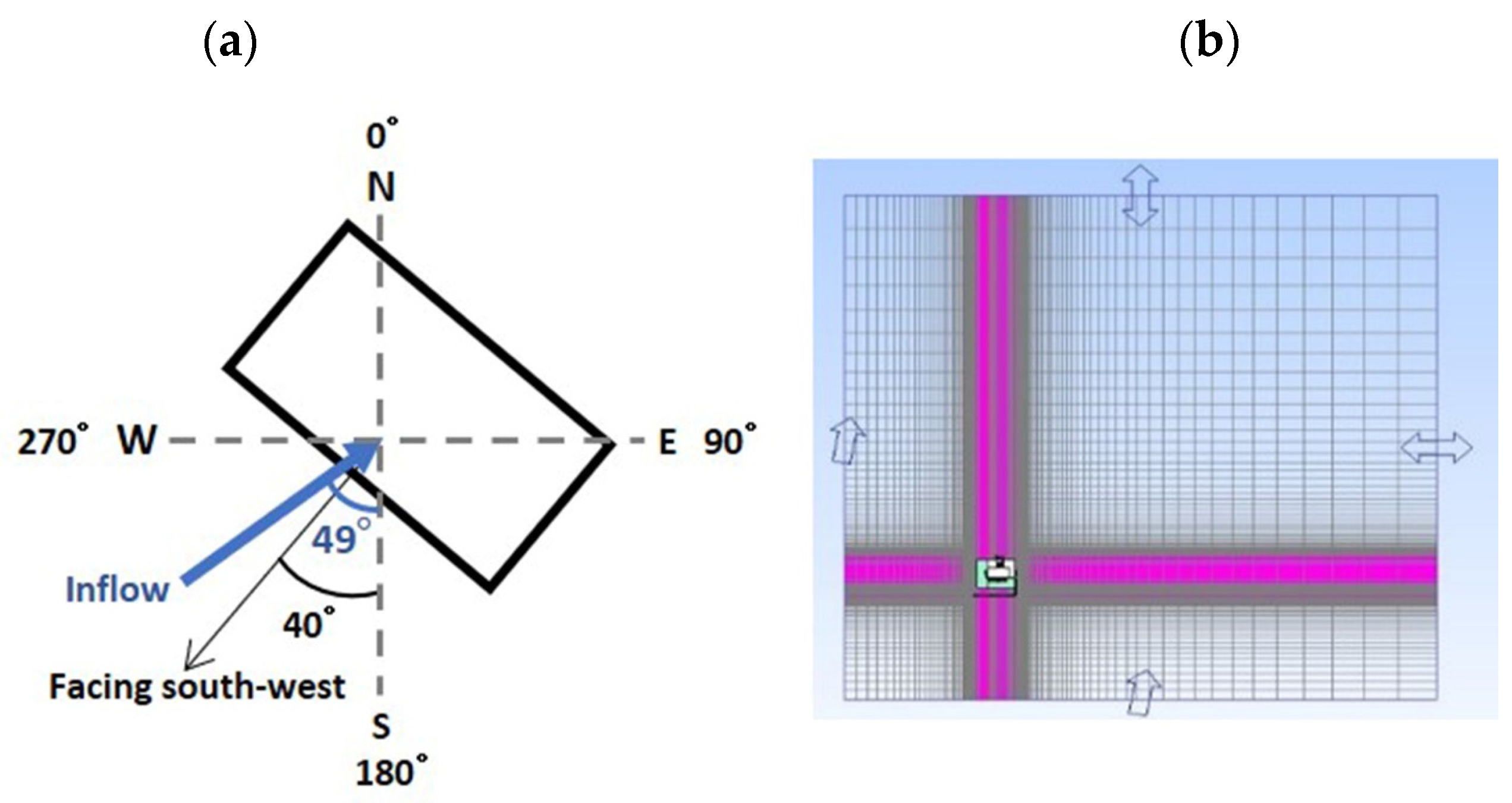
3.1.2. Flow Conditions
3.1.3. Thermal Conditions
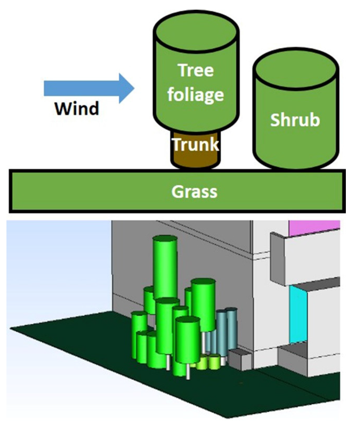
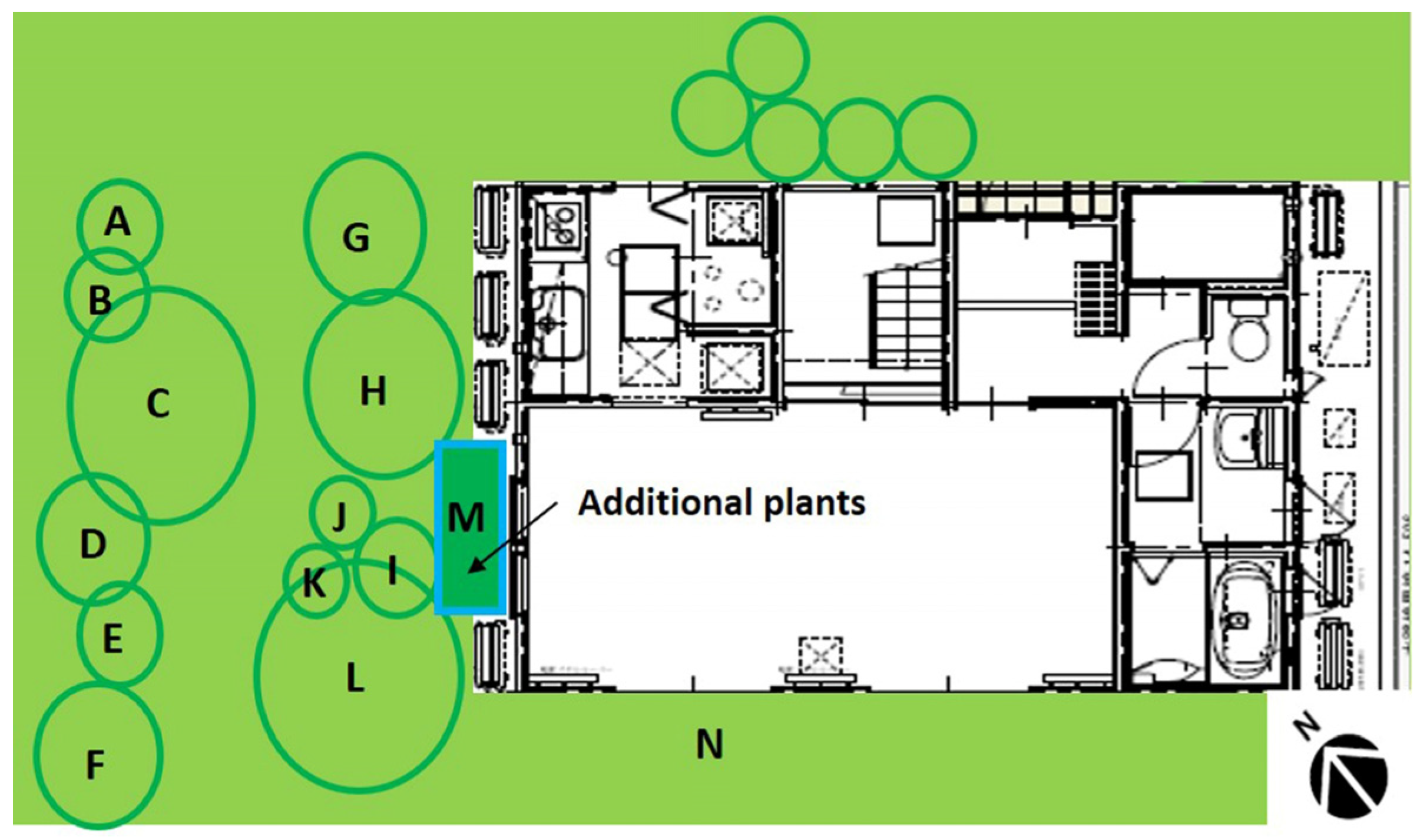
3.1.4. Canopy Setting
3.1.5. Humidity Conditions
3.2. Validation Results
4. Result and Discussion
4.1. Investigation of Cooling Effect by Passive Cooling Design
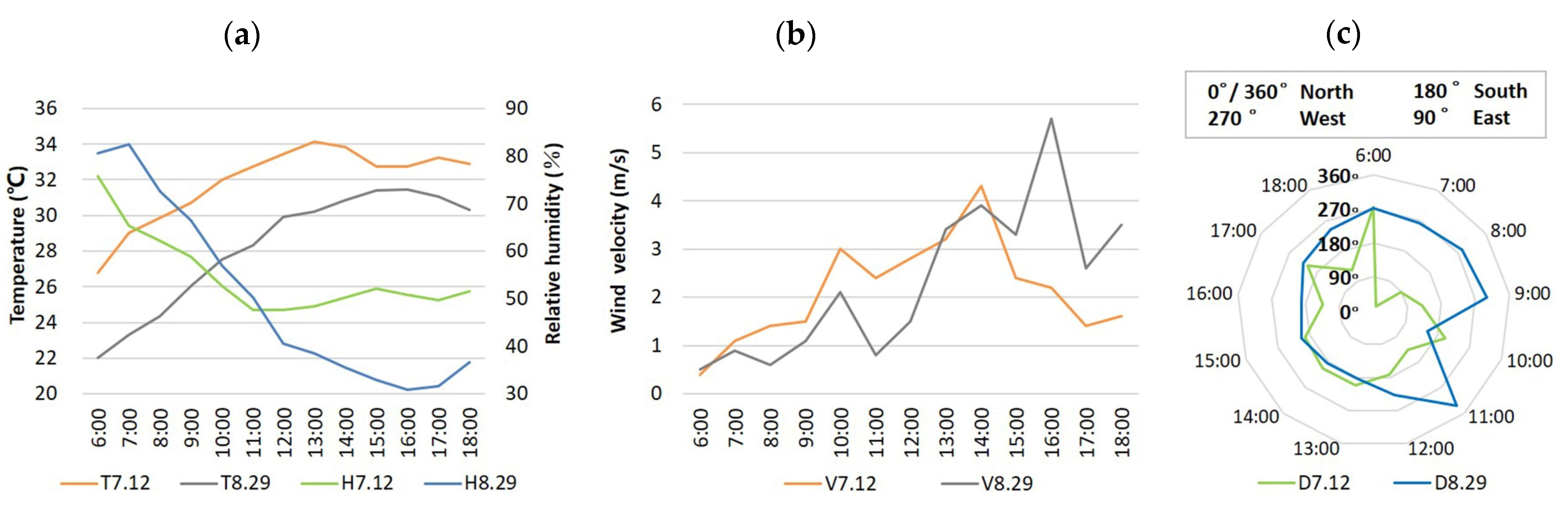
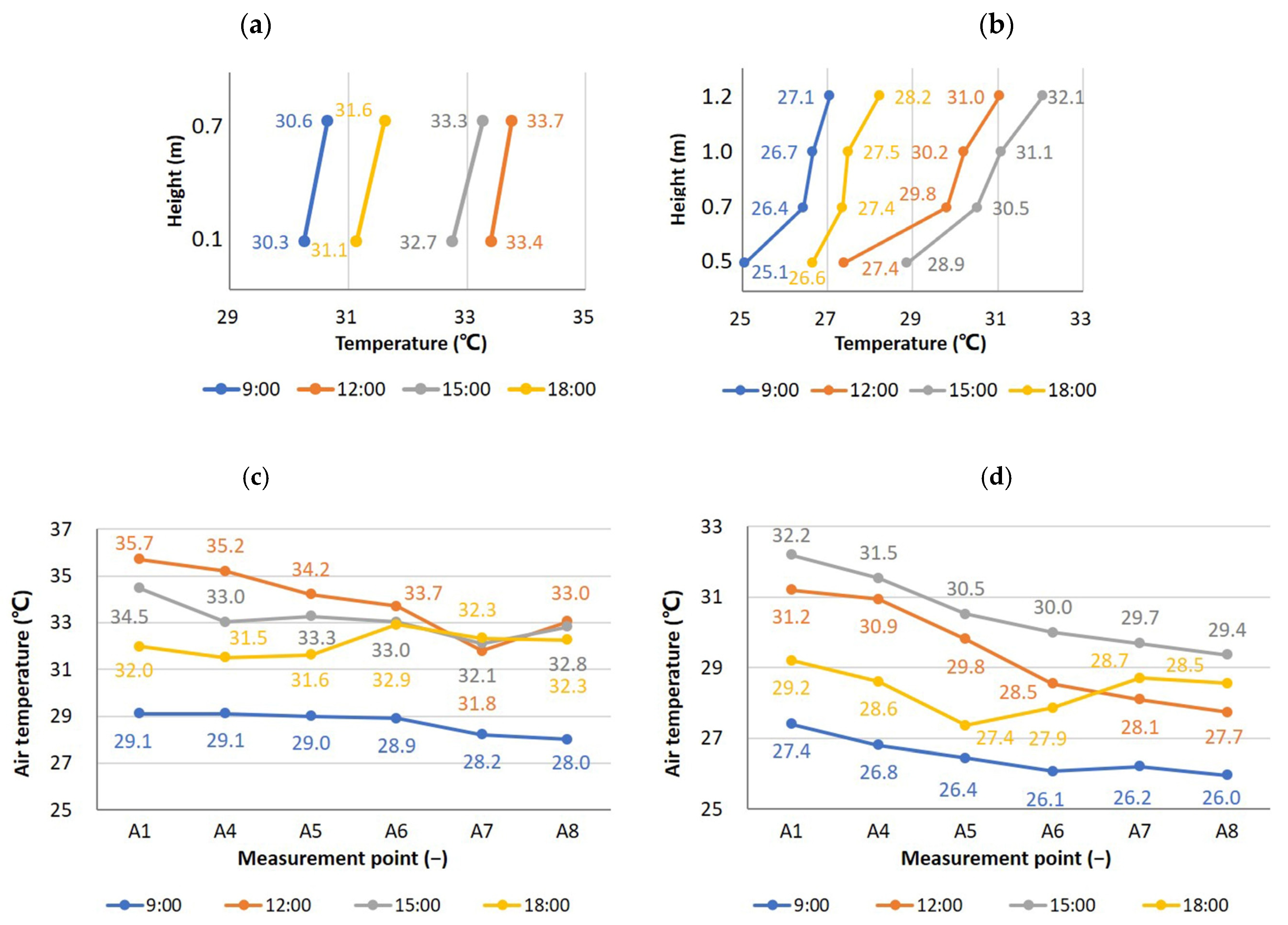
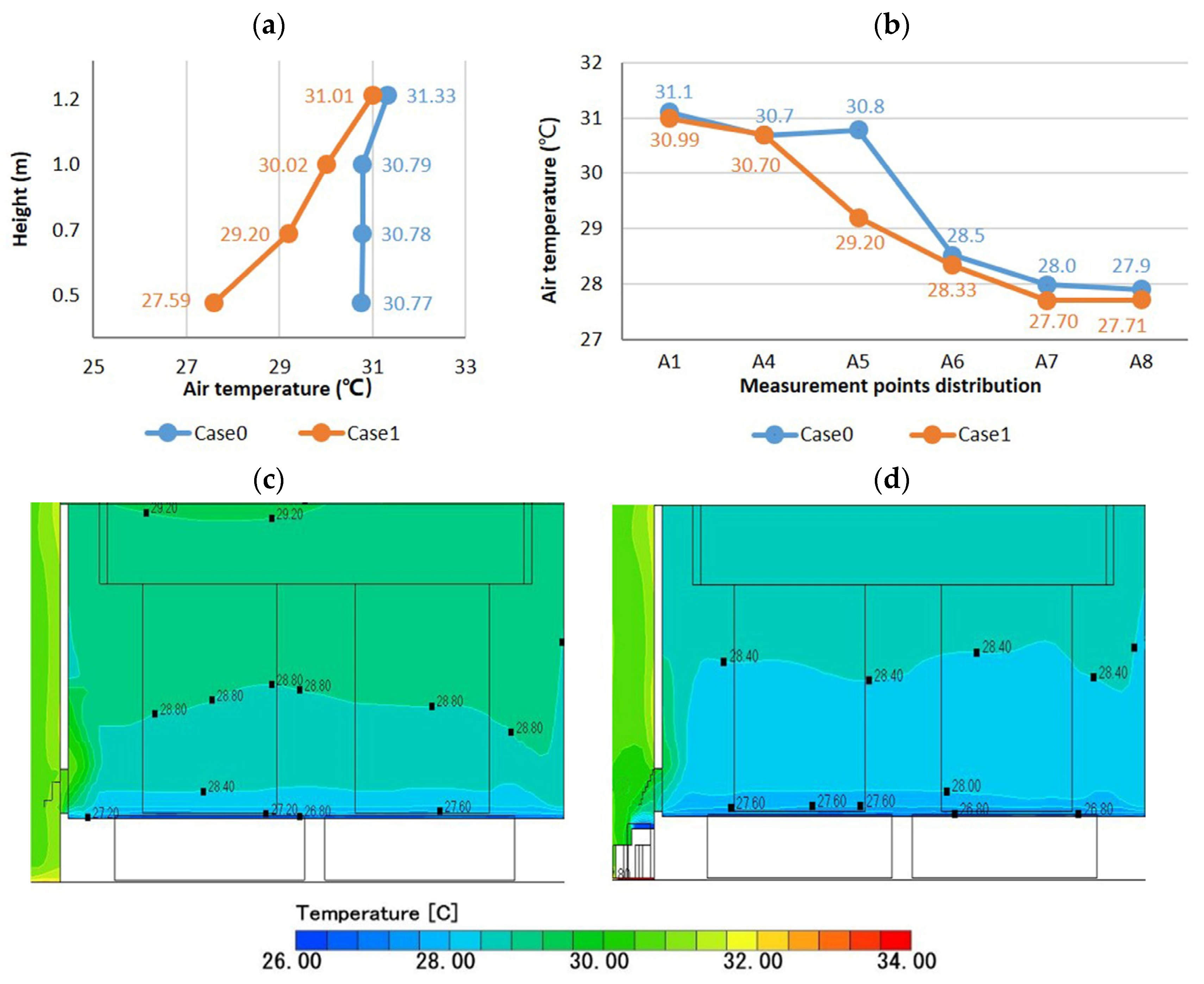
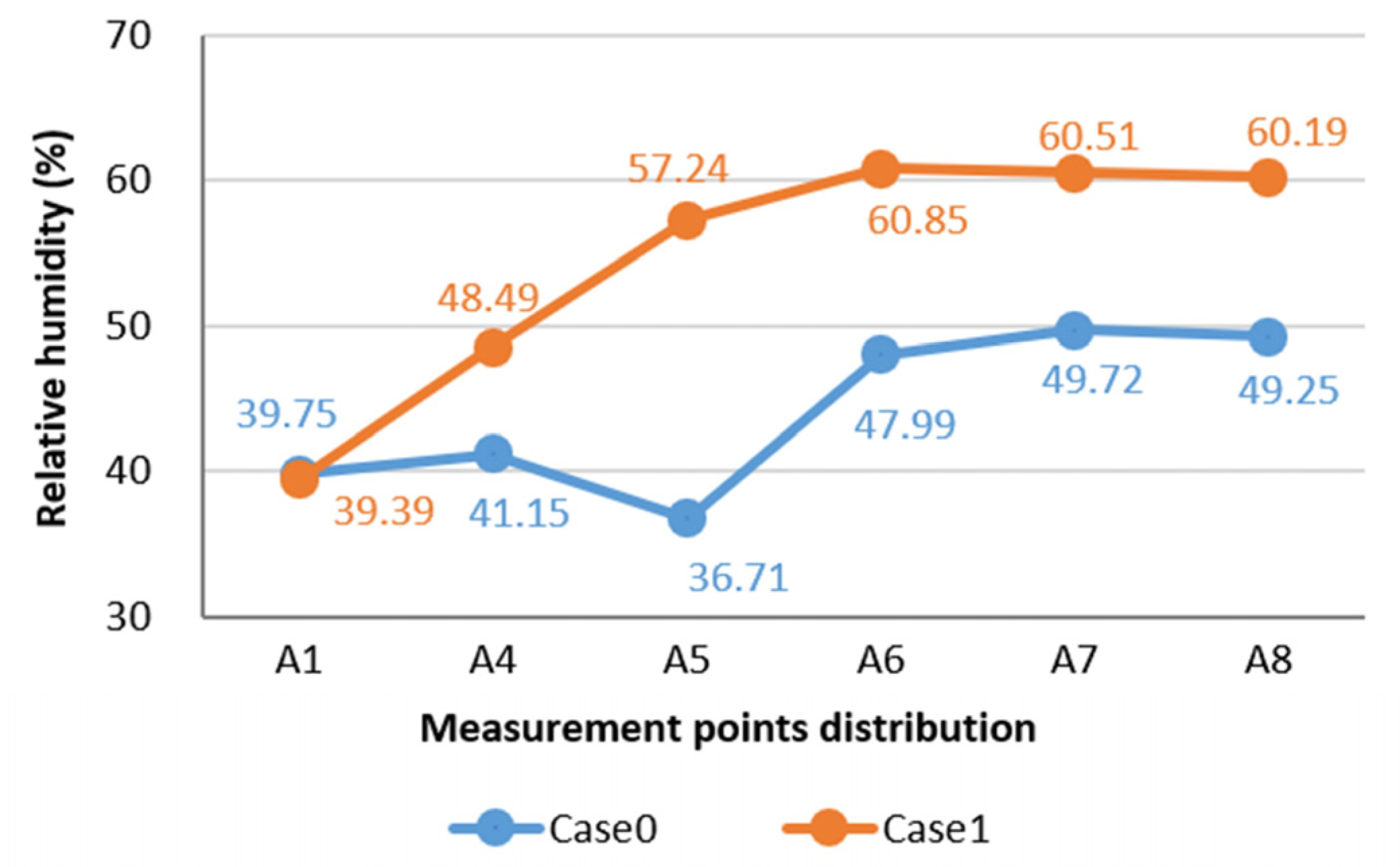
4.1.1. Experiment Results and Analysis: Temperature and Humidity Distribution
4.1.2. Simulation Results and Analysis: Temperature, Flow, Humidity, and Standard Effective Temperature* (SET*)
4.2. Sensitivity Analysis on the Floor-Level Window Design
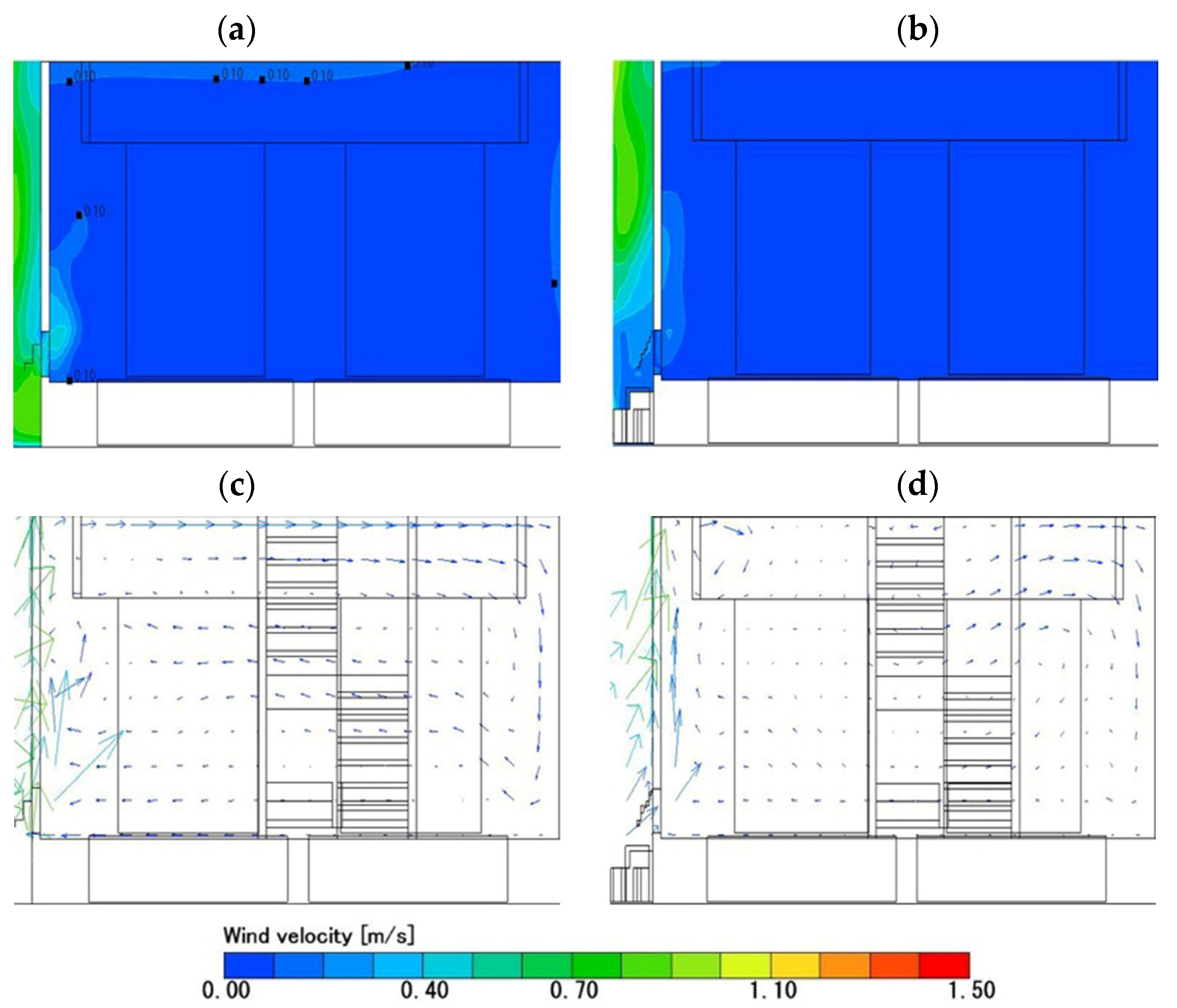
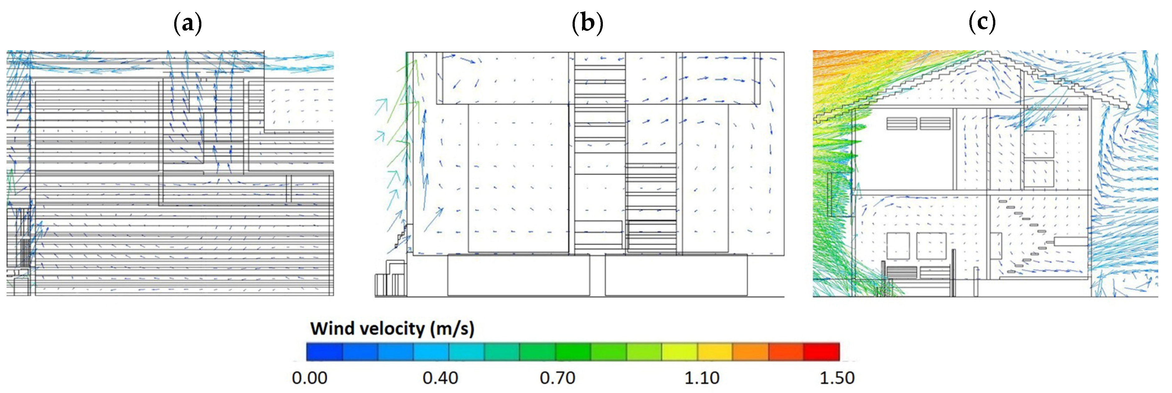
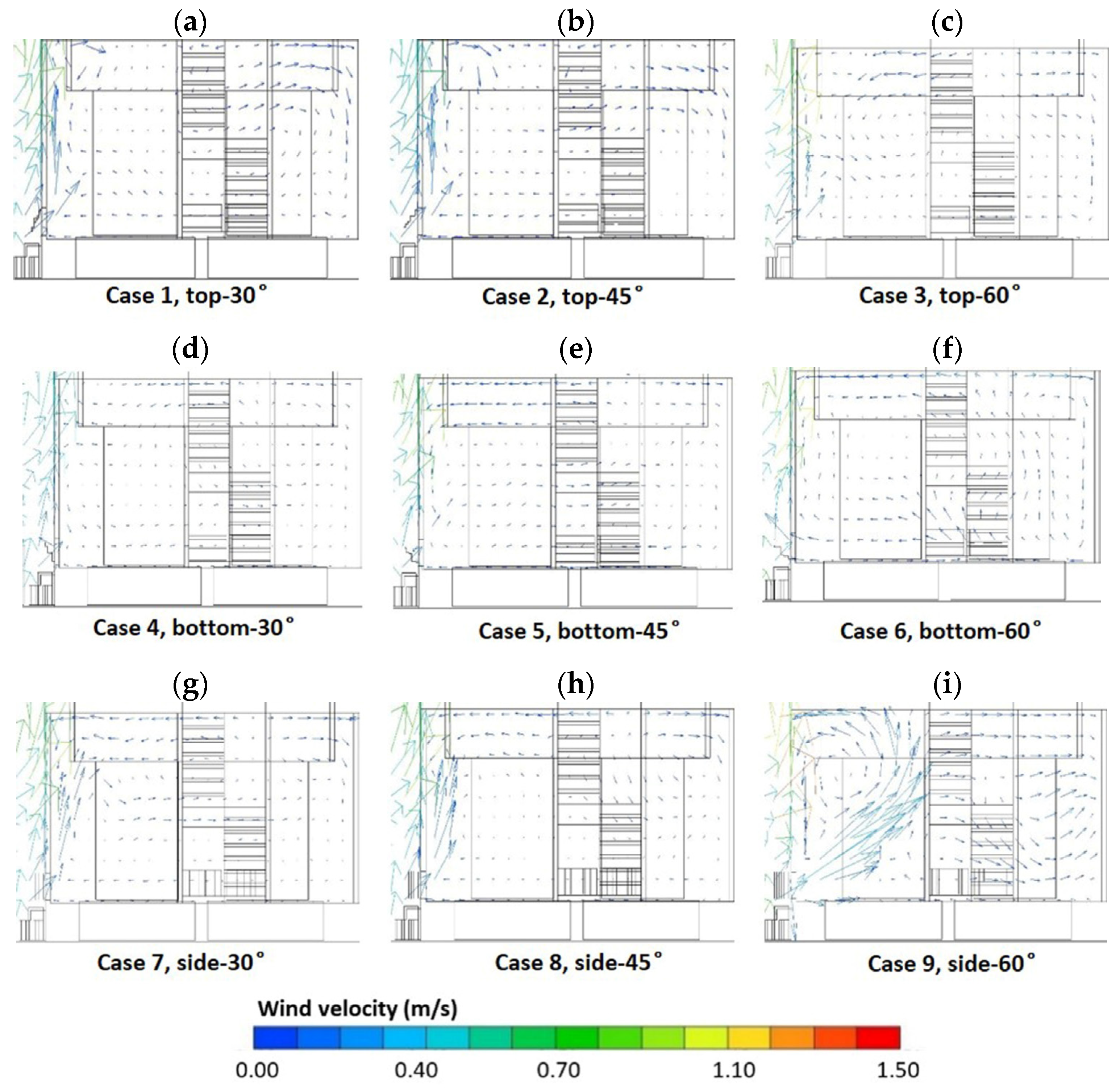
4.2.1. Simulation Results and Analysis: Flow Distribution
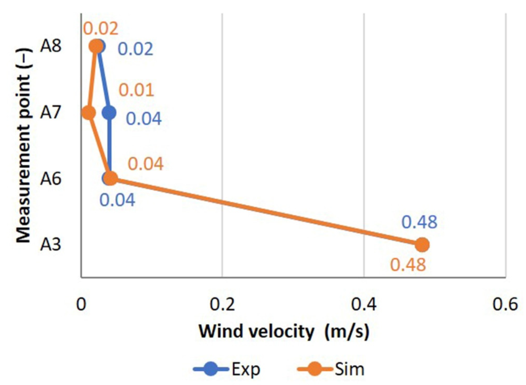
4.2.2. Simulation Results and Analysis: Wind Velocity
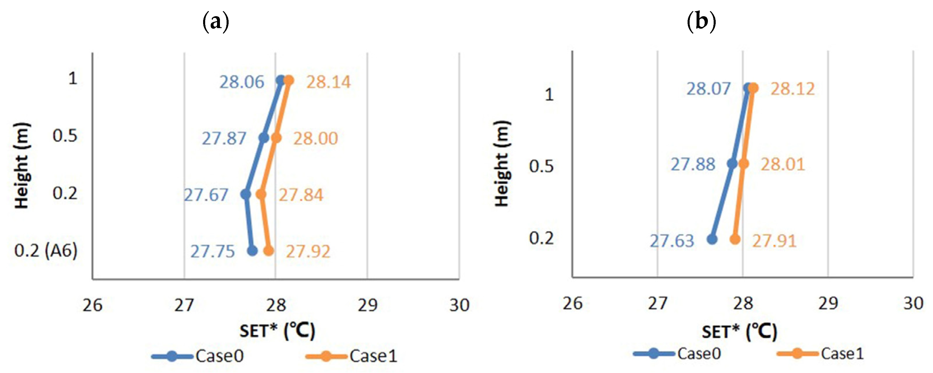
4.2.3. Simulation Results and Analysis: Standard Effective Temperature* (SET*)
5. Conclusions
- In this study, we proposed a ventilation model that combined a passive cooling design with natural ventilation, using floor-level windows. The passive cooling design consisted of a water retentive block, plants, and dripping pipes placed in front of the floor-level windows. Based on the results of the field experiment and CFD-based simulation, we conclude that the passive cooling design reduced the semi-outdoor and indoor temperatures, and increased the relative humidity.
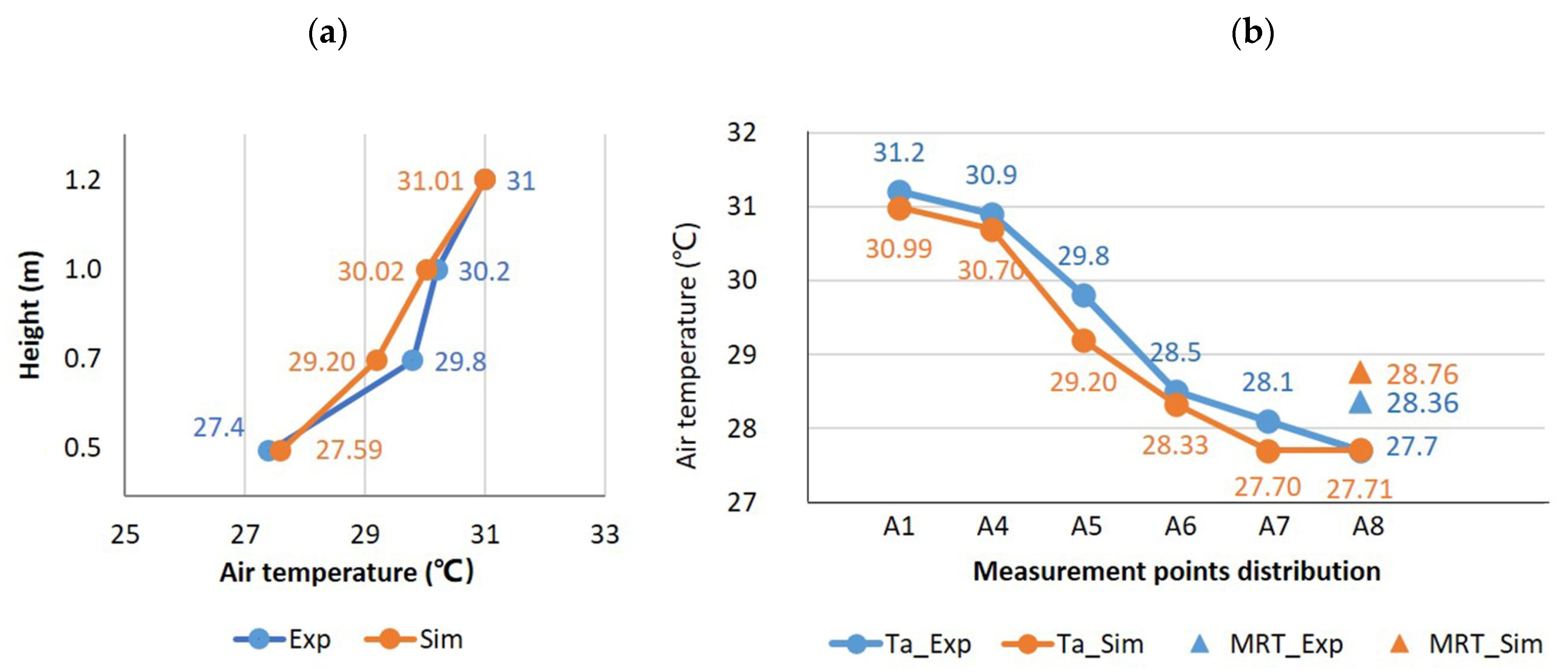
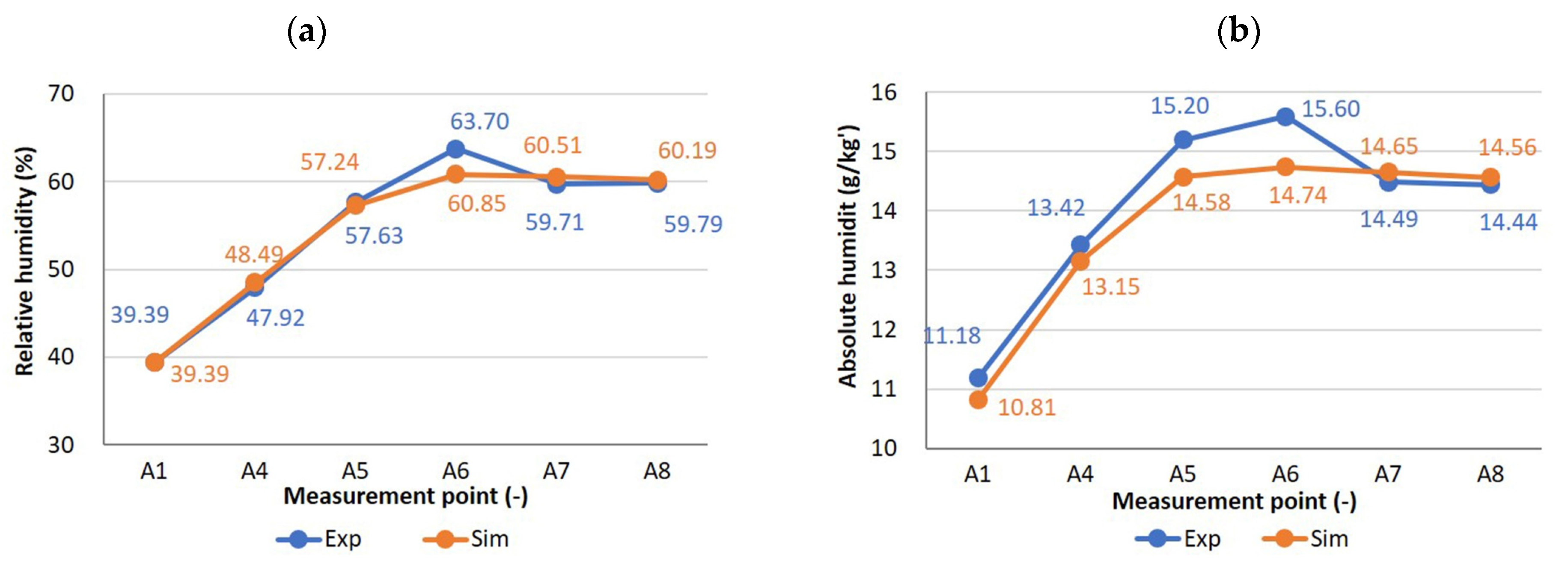
- The CFD-based simulation model applied in this study was validated by a measurement-to-simulation comparison on a late summer day (air temperature up to 32 °C with a relatively high-speed wind up to around 6 m/s), and was proved to be valid to test the effect of passive cooling design in terms of air temperature, wind velocity, humidity and MRT with acceptable errors.
- With the floor-level windows and skylight open during the ventilation period, a flow path formed inside that inflow, with the flow mainly originating from the western floor-level windows and the skylight, to then escape from the northern floor-level windows.
- Regarding the type of floor-level windows, the side hung type performed better in introducing airflow inside the house; side hung windows with an opening angle of 60° appear to be the best choice, in terms of the increasing of ventilation, since the wind velocity reached 0.4 m/s in the center of the living room. However, the indoor thermal comfort was not improved (SET*s mainly of around 27 °C and 28 °C, above the comfort range) by enhancing the ventilation. To solve this problem, future studies should discuss and explore the configuration of the passive cooling design near floor-level windows.
Author Contributions
Funding
Conflicts of Interest
References
- NASA Earth Obeservatory. World of Change: Global Temperatures. 2022. Available online: https://earthobservatory.nasa.gov/world-of-change/global-temperatures (accessed on 20 June 2022).
- Arakawa, R.; Tsutsumi, J.; Nakamatsu, R. A study on historical change of residential houses and their indoor thermal environment in subtropical Okinawa. Trans. Archit. Inst. Jpn. 2007, 618, 109–114. [Google Scholar]
- International Energy Agency (IEA). The Future of Cooling: Opportunities for Energy-Efficient Air Conditioning; International Energy Agency (IEA): Paris, France, 2018. [Google Scholar]
- Cook, J. Passive Cooling; Arizona State Univ.: Tempe, AZ, USA, 1989. [Google Scholar]
- Givoni, B. Performance and applicability of passive and low-energy cooling systems. Energy Build. 1991, 17, 177–199. [Google Scholar] [CrossRef]
- Abro, R.S. Recognition of passive cooling techniques. Renew. Energy 1994, 5, 1143–1146. [Google Scholar] [CrossRef]
- Chen, J.; Brager, G.S.; Augenbroe, G.; Song, X. Impact of outdoor air quality on the natural ventilation usage of commercial buildings in the US. Appl. Energy 2019, 235, 673–684. [Google Scholar] [CrossRef]
- Kamal, M.A. An Overview of Passive Cooling Techniques in Buildings: Design Concepts and Architectural Interventions. Civ. Eng. Archit. 2012, 55, 84–97. [Google Scholar]
- Geros, V.; Santamouris, M.; Tsangrasoulis, A.; Guarracino, G. Experimental evaluation of night ventilation phenomena. Energy Build. 1999, 29, 141–154. [Google Scholar] [CrossRef]
- Chen, J.; Saunders, S.C.; Crow, T.R.; Naiman, R.J.; Brosofske, K.D.; Mroz, G.D.; Brookshire, B.L.; Franklin, J.F. Microclimate in Forest Ecosystem and Landscape Ecology: Variations in local climate can be used to monitor and compare the effects of different management regimes. Bioscience 1999, 49, 288–297. [Google Scholar] [CrossRef] [Green Version]
- Yang, A.S.; Juan, Y.H.; Wen, C.Y.; Chang, C.J. Numerical simulation of cooling effect of vegetation enhancement in a subtropical urban park. Appl. Energy 2017, 192, 178–200. [Google Scholar] [CrossRef]
- Wong, P.P.Y.; Lai, P.C.; Low, C.T.; Chen, S.; Hart, M. The impact of environmental and human factors on urban heat and microclimate variability. Build. Environ. 2016, 95, 199–208. [Google Scholar] [CrossRef] [Green Version]
- Matsumoto, F.; Ichinose, T.; Shiraki, Y.; Lee, L. Climatological study about effect of ventilation by a large restoration of inner-city river—A case of Cheong-Gye Stream in Seoul, South Korea. Jpn. J. Biometeorol. 2009, 46, 69–80. [Google Scholar]
- Del Rio, M.A.; Asawa, T.; Hirayama, Y.; Sato, R.; Ohta, I. Evaluation of passive cooling methods to improve microclimate for natural ventilation of a house during summer. Build. Environ. 2019, 149, 275–287. [Google Scholar] [CrossRef]
- Lee, T.C.; Asawa, T.; Kawai, H.; Sato, R.; Hirayama, Y.; Ohta, I. Multipoint measurement method for air temperature in outdoor spaces and application to microclimate and passive cooling studies for a house. Build. Environ. 2017, 114, 267–280. [Google Scholar] [CrossRef]
- Rouleau, J.; Gosselin, L. Probabilistic window opening model considering occupant behavior diversity: A data-driven case study of Canadian residential buildings. Energy 2020, 195, 116981. [Google Scholar] [CrossRef]
- Toe, D.H.C.; Kubota, T. Comparative assessment of vernacular passive cooling techniques for improving indoor thermal comfort of modern terraced houses in hot–humid climate of Malaysia. Sol. Energy 2015, 114, 229–258. [Google Scholar] [CrossRef]
- Xie, X.; Sahin, O.; Luo, Z.; Yao, R. Impact of neighbourhood-scale climate characteristics on building heating demand and night ventilation cooling potential. Renew. Energy 2020, 150, 943–956. [Google Scholar] [CrossRef]
- Sunaga, N.; Onodera, H.; Kumakura, E.; Ogino, T. Actual state data and methods for improving the indoor thermal environment of apartment houses in the hot–humid regions of Japan. J. Hous. Res. Found. 2019, 45, 83–94. [Google Scholar]
- Horikoshi, T. Basic Principle of a Buffer Zone between Indoor and Outdoor as Environmental Control Devices in Dwelling Houses. Trans. Soc. Heat. Air Cond. Sanit. Eng. Jpn. 2017, 265–268. [Google Scholar]
- Yuta, I.; Kengo, K.; Ko, N. The study of the architectural style of tea house by the multivariable analysis using the data of the presence of absence of elements. J. Archit. Plan. 2015, 80, 2365–2373. [Google Scholar]
- Saito, M.; Nasu, S. Luminous Performance of Ji-mado as a Daylighting System In Snowy Region. In Proceedings of the 2005 World Sustainable Building Conference, Tokyo, Japan, 27–29 September 2005; pp. 27–29. [Google Scholar]
- Lee, T.C.; Yoon, S.H. A measurement on cold storage of phase change material on the floor of the building with night natural ventilation. J. Archit. Inst. Korea 2021, 37, 151–156. [Google Scholar]
- Jiang, L.; Tang, M. Thermal analysis of extensive green roofs combined with night ventilation for space cooling. Energy Build. 2017, 156, 238–249. [Google Scholar] [CrossRef]
- Lai, D.; Liu, W.; Gan, T.; Liu, K.; Chen, Q. A review of mitigating strategies to improve the thermal environment and thermal comfort in urban outdoor spaces. Sci. Total Environ. 2019, 661, 337–353. [Google Scholar] [CrossRef] [PubMed]
- Seina, U.; Onshi, A.; Masayuki, S. Evaluation and examination of measures toward promoting planting green at detached houses. J. Jpn. Soc. Civ. Eng. Ser. G 2016, 72, I-109–I-117. [Google Scholar]
- Motofumi, M.; Akira, H.; Takashi, A.; Yoshie, I. An experiment on the fundamental performance of an evaporative cooling pavement system during summer:development of an evaporative cooling pavement system and cooling effect simulation model forurban thermal environment Part1. J. Jpn. Soc. Civ. Eng. Ser. G 2006, 71, 51–58. [Google Scholar]
- He, J.; Hoyano, A. Numerical Analysis on the Mitigating Effects of Evaporative Cooling Strategies on the Heat Island Potential for Urban Blocks. J. Heat Isl. Inst. Int. 2007, 2, 6–13. [Google Scholar]
- Mayumi, Y.; Hiroyuki, T.; Koichi, N. Reproducibility of the Atmosphere-Subsurface-Coupled Hydrothermal Environment Model. J. Heat Isl. Inst. Int. 2010, 5, 24–32. [Google Scholar]
- Architectural Institute of Japan. AIJ Benchmarks for Validation of CFD Simulations Applied to Pedestrian Wind Environment around Buildings Architectural Institute of Japan; Architectural Institute of Japan: Tokyo, Japan, 2016; ISBN 9784818950016. [Google Scholar]
- Porras-Amores, C.; Mazarrón, F.R.; Cañas, I.; Villoría Sáez, P. Natural ventilation analysis in an underground construction: CFD simulation and experimental validation. Tunn. Undergr. Space Technol. 2019, 90, 162–173. [Google Scholar] [CrossRef]
- Xiao, H.; Cinnella, P. Quantification of model uncertainty in RANS simulations: A review. Prog. Aerosp. Sci. 2019, 108, 1–31. [Google Scholar] [CrossRef] [Green Version]
- Ryo, S.; Masanari, U.; Tatsuo, N. Effective Evaluation of Natural Ventilation System. Trans. Soc. Heat. Air Cond. Sanit. Eng. Jpn. 2017, 4, 1–4. [Google Scholar]
- Wang, H.; Chen, Q. Modeling of the impact of different window types on single-sided natural ventilation. Energy Procedia 2015, 78, 1549–1555. [Google Scholar] [CrossRef] [Green Version]
- Heiselberg, P.; Svidt, K.; Nielsen, P.V. Characteristics of airflow from open windows. Build. Environ. 2001, 36, 859–869. [Google Scholar] [CrossRef]
- Liu, T.; Lee, W.L. Using response surface regression method to evaluate the influence of window types on ventilation performance of Hong Kong residential buildings. Build. Environ. 2019, 154, 167–181. [Google Scholar] [CrossRef]
- Zhai, Y.; Wang, Y.; Huang, Y.; Meng, X. A multi-objective optimization methodology for window design considering energy consumption, thermal environment and visual performance. Renew. Energy 2019, 134, 1190–1199. [Google Scholar] [CrossRef]
- Von Grabe, J. Flow resistance for different types of windows in the case of buoyancy ventilation. Energy Build. 2013, 65, 516–522. [Google Scholar] [CrossRef]
- Amaral, A.R.; Rodrigues, E.; Gaspar, A.R.; Gomes, Á. A thermal performance parametric study of window type, orientation, size and shadowing effect. Sustain. Cities Soc. 2016, 26, 456–465. [Google Scholar] [CrossRef] [Green Version]
- Kazuo, F.; Hiroshi, I.; Shigeru, G.; Satoshi, A.; Junji, S. An experiment on SET* and thermal comfort of Japanese. Trans. Soc. Heat. Air Cond. Sanit. Eng. Jpn. 1993, 18, 139–147. [Google Scholar]
- Kenichi, H. Discussion on error of PMV and comfort range under the approximate method between air temperature and MRT. Trans. Soc. Heat. Air Cond. Sanit. Eng. Jpn. 2006, 109, 29–32. [Google Scholar]
- Del Rio, M.A.; Asawa, T.; Hirayama, Y. Modeling and validation of the cool summer microclimate formed by passive cooling elements in a semi-outdoor building space. Sustainability 2020, 12, 5360. [Google Scholar] [CrossRef]
- Liu, J.; Heidarinejad, M.; Pitchurov, G.; Zhang, L.; Srebric, J. An extensive comparison of modified zero-equation, standard k-ε, and LES models in predicting urban airflow. Sustain. Cities Soc. 2018, 40, 28–43. [Google Scholar] [CrossRef]
- Du, Y.; Mak, C.M.; Ai, Z. Modelling of pedestrian level wind environment on a high-quality mesh: A case study for the HKPolyU campus. Environ. Model. Softw. 2018, 103, 105–119. [Google Scholar] [CrossRef]
- McAdams, W.H.; William, H. Heat Transmission, 3rd ed.; McGraw-Hill: New York, NY, USA, 1954. [Google Scholar]
- Hosoi, F.; Omasa, K. Estimating vertical leaf area density profiles of tree canopies using three-dimensional portable lidar imaging. Scanning 2009, 64, 151–158. [Google Scholar]
- Nemoto, H. Research on the Passive Cooling Effect on Residential House by Adjustment of Plants on Microclimate and Natural Ventilation; Tokyo Institute of Technology: Yokohama, Japan, 2014. [Google Scholar]
- Kenji, K.; Masamiki, O.; Ken-ichi, N. Wind tunnel experiments on drag coefficient of trees with the leaf area density as a reference area. J. Environ. Eng. 2004, 578, 71–77. [Google Scholar]
- Asawa, T.; Fujiwara, K.; Hoyano, A.; Shimizu, K. Convective heat transfer coefficient of crown of Zelkova Serrata. J. Environ. Eng. 2016, 81, 235–245. [Google Scholar] [CrossRef] [Green Version]
- Kiyono, T.; Asawa, T.; Hoyano, A.; Shimizu, K. Weighing whole tree transpiration rate of urban trees and analysis of trees Morpho-Physiological effects. J. Environ. Eng. 2015, 80, 599–608. [Google Scholar] [CrossRef] [Green Version]
- SIMTEQ Engineering (Pty) Ltd. Tutorials of Cradle CFD 2020-csSTREAM. Available online: https://simteq.co.za/blog/cradle-getting-started/ (accessed on 20 June 2022).
- Tetens, O. Uber einige meteorologische Begriffe. Z. Geophys. 1930, 6, 297–309. [Google Scholar]


| Type | Top Hung Window (30°) |
|---|---|
| Size | 800 × 400 mm |
| Total amount | 2 in the west, 2 in the north |
| Heat transmission coefficient | 2.91 W/m2·K |
| 0.7 |
| Experiment | 12 July (Case A) | 29 August (Case B) |
|---|---|---|
| Setting conditions |
|
|
| Temperature | Relative Humidity | Wind Velocity | ||
|---|---|---|---|---|
| Location and vertical distribution to measure the data | A1, A2, A4 | GL + 0.1 m, 1.1 m | GL + 1.1 m | - |
| A3 | GL + 0.1 m, 0.7 m, 1.1 m | - | GL + 0.7 m | |
| A5 | GL + 0.5 m, 0.7 m, 1 m, 1.2 m; | GL + 0.7 m | - | |
| A6 | FL + 0.2 m | FL + 0.2 m | FL + 0.2 m | |
| A7 | FL + 0 m, 0.1 m, 0.5 m, 1.1 m, 1.8 m, 2.3 m, and ceiling surface | FL + 1.1 m | FL + 1.1 m | |
| A8 | FL + 0 m, 0.1 m, 0.5 m, 1.1 m, 1.8 m, 2.3 m, and ceiling surface | FL + 1.1 m | FL + 1.1 m | |
| Instrument | Air temperature: 0.1-mmФ T-type thermocouple with multipoint measurement method Surface temperature: 0.3-mmФ T-type thermocouple MRT: 0.1-mmФ T-type thermocouple inside a globe thermometer (FL+ 1 m at A8 only) | Resistance change type (TDK, CHS-UPS) | A3: 3D ultrasonic anemometers A6, A7, A8: KAJIO, DA0600 | |
| Window Type | Top Hung | Bottom Hung | Side Hung |
|---|---|---|---|
| Size | 800 × 400 mm | 400 mm | 400 × 400 mm (2) |
| Figure of one unit | 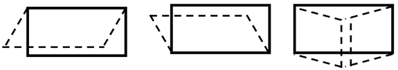 | ||
| Window Type | Opening Angle | Case |
|---|---|---|
| Top hung window | 30° | Case 1 |
| 45° | Case 2 | |
| 60° | Case 3 | |
| Bottom hung window | 30° | Case 4 |
| 45° | Case 5 | |
| 60° | Case 6 | |
| Side hung window | 30° | Case 7 |
| 45° | Case 8 | |
| 60° | Case 9 |
| Domain | 174.5 × 174.5 × 41.5 m | |
| Mesh | 251 × 269 × 165 = 11,140,635 | |
| Turbulence model | Standard k-ε model | |
| Inflow boundary | Direction | SW (229°) |
| Velocity | 1.5 m/s (Basic height: 8.3 m) | |
| Environment | Ⅲ: Urban area formed by small buildings | |
| ZG: 450 m α: 0.2 | ||
| Outflow boundary | Ymax and Xmin: No pressure | |
| Wall boundary | Zmin: No slip; Zmax: Free slip | |
| Scheme for convection terms | QUICK scheme | |
| Cycle | Stable analysis, 500 cycle | |
| Indoor Surface Temperature (°C) | Outdoor Surface Temperature (°C) | ||
|---|---|---|---|
| Indoor wall (South, East) | 27.8 | Outdoor wall (upward of West wall) | 36.54 |
| Indoor wall (North, West) | 28.04 | Outdoor wall (downward of West wall) | 34.89 |
| Ceiling of the 1st floor | 26.47 | Outdoor wall (North, East wall) | 34 |
| Ground of the 1st floor | 27.59 | Outdoor wall (South wall) | 37 |
| Sweeping windows | 30.34 | Roof | 42 |
| Water retentive block | 26 | ||
| Ceramic grid panel | 34 | ||
| Outside step (West, East) | 32, 52 | ||
| Outdoor louver | 23.8 | ||
| Outdoor shading | 47 | ||
| Types | Number Shown in Figure 8 | Cd | LAD (m2/m3) | Temperature (°C) |
|---|---|---|---|---|
| Evergreen shrub | A | 0.5 | 5–6 | 29.15 |
| Evergreen tree | D, I, L | 0.6 | 5–6 | 34.23 |
| Delicious shrub | B, C, F, J, K | 0.6 | 3–5 | 29.15 |
| Delicious tree | E, G, H | 0.6 | 3–5 | 34.23 |
| Grass | N | 0.8 | 7 | 37 |
| Boxwood | M | 0.5 | 5–6 | 28 |
| Index | MSE | RMSE | R2 |
|---|---|---|---|
| TV | 0.11 °C | 0.33 °C | 0.95 |
| TH | 0.10 °C | 0.32 °C | 0.98 |
| Wind velocity | 0.0004 m/s | 0.02 m/s | 0.99 |
| Relative humidity | 2.5% | 16% | 0.98 |
| Absolute humidity | 0.23 g/kg | 0.48 g/kg | 0.94 |
Publisher’s Note: MDPI stays neutral with regard to jurisdictional claims in published maps and institutional affiliations. |
© 2022 by the authors. Licensee MDPI, Basel, Switzerland. This article is an open access article distributed under the terms and conditions of the Creative Commons Attribution (CC BY) license (https://creativecommons.org/licenses/by/4.0/).
Share and Cite
Qin, B.; Xu, X.; Asawa, T.; Zhang, L. Experimental and Numerical Analysis on Effect of Passive Cooling Methods on an Indoor Thermal Environment Having Floor-Level Windows. Sustainability 2022, 14, 7880. https://doi.org/10.3390/su14137880
Qin B, Xu X, Asawa T, Zhang L. Experimental and Numerical Analysis on Effect of Passive Cooling Methods on an Indoor Thermal Environment Having Floor-Level Windows. Sustainability. 2022; 14(13):7880. https://doi.org/10.3390/su14137880
Chicago/Turabian StyleQin, Beilei, Xi Xu, Takashi Asawa, and Lulu Zhang. 2022. "Experimental and Numerical Analysis on Effect of Passive Cooling Methods on an Indoor Thermal Environment Having Floor-Level Windows" Sustainability 14, no. 13: 7880. https://doi.org/10.3390/su14137880
APA StyleQin, B., Xu, X., Asawa, T., & Zhang, L. (2022). Experimental and Numerical Analysis on Effect of Passive Cooling Methods on an Indoor Thermal Environment Having Floor-Level Windows. Sustainability, 14(13), 7880. https://doi.org/10.3390/su14137880