Dynamic Relationships between Seafood Exports, Exchange Rate and Industrial Upgrading

Abstract

Few studies have examined the relationship between seafood export performance and exchange rate fluctuations. This paper investigates the short and long-term relationship between variables and the effect of currency depreciation on investment in industrial upgrading in the Namibian seafood industry. Employing the Johansen cointegration technique and a vector error correction model (VECM) on quarterly data from 2008 to 2020, we find that investment in industrial upgrading has a higher impact on exports than exchange rate fluctuations. Therefore, investment in industrial upgrading plays a significant role in mitigating the negative impact of exchange rate volatility. Key policy implications include the need to take advantage of currency depreciation to mitigate challenges to investment in industrial upgrading by increased budgetary allocations.

1. Introduction

The export performance of seafood-dependent economies, particularly in developing countries, is facing unprecedented shocks due to inadequate value addition, stringent safety standards and regulations and financial constraints to enhance competitive exports [1,2,3]. The continued ability to export competitive products required for improved export performance underpins the economic development of seafood-dependent economies. Moreover, exports must have long-term export sustainability [4]. Therefore, industrial upgrading is essential for export performance among the many determinants of competitive exports. Processed seafood exports are highly reliant on industrial upgrading in the form of a stepwise development from simple manufacturing skills to complicated tasks. However, most developing countries that export seafood cannot upgrade their export processing facilities [5], making market access difficult and the competitiveness of their products uncertain [6]. Due to the possibility of an increase in demand for processed seafood as a result of dietary changes, convenience, packaging and preservation methods and availability [7], inadequate value addition in the form of export processing may hinder export performance [2,8].

Constraints on industrial upgrading and the rising demand for seafood products have revealed two major concerns. First, inadequate funding may impede industrial upgrading, especially in developing nations, resulting in insufficient value addition or an increase in unprocessed exports, with consequences for trade benefits [9,10]. Second, the increasing demand for unprocessed seafood may encourage reprocessing trade [11]. In this case, exporters may lose potential export earnings if they fail to add value before exporting.

In an effort to address the abovementioned issues, the causal relationships between industrial upgrading, seafood export and exchange rate volatility have received growing attention in recent years. Existing research is, however, inconclusive regarding the direction of causal relationships. On the one hand, some studies describe a supply-driven relationship and argue that the cost of industrial upgrades is driven by exchange rate volatility, resulting in a rise in the cost of upgrades, with reverberating effects on export performance [12,13,14,15]. On the other hand, others explain that demand-driven causation exists where unprocessed seafood exports are likely to negatively impact seafood export performance and revenue, leading to increased costs of industrial upgrades to meet import demands [16,17,18]. These studies argue that uncompetitive exports tend to limit market access, increasing the need for industrial upgrades and, as a result, the cost of upgrades. Therefore, whether the causal relationships between export, industrial upgrading and exchange rate are demand-driven or supply-driven remains inconclusive.

Given the impact of industrial upgrading on seafood export performance and global food security [19] and the increasing policy emphasis on certification and standards, it is crucial to determine the relationship [20]. Few empirical studies [12,21] have examined the relationship between export performance and exchange rate, but they have not accounted for the most influential export performance determinant, industrial upgrading. Investment in seafood industrial upgrading has been on a significant rise in Namibia. The medium expenditure framework 2009 (https://www.npc.gov.na/publications, accessed on 23 May 2022) shows that between 2008 to 2020, Namibia’s investment in industrial upgrading increased by 74%, while processed seafood exports increased by 88% (see Figure 1). However, the causal relationship between the variables and the role of the exchange rate on industrial upgrading is unknown. What is the effect of exchange rate volatility, specifically currency depreciation, on industrial upgrading and what is the impact on the long-term processed export sustainability of the Namibian seafood industry? Consequently, this study uses investment and development expenditure in industrial upgrading to examine the relationship between industrial upgrading and export performance and exchange rate in the Namibian seafood industry.

Using a vector error correction model (VECM) and graphical analysis-impulse response function in a multivariate dynamic framework, we employ a time series approach to analyse the causal relationships. The seafood exports under consideration include the principal export species, hake and horse mackerel, classified according to the 6-digit HS codes as fillets-fresh, chilled or frozen, prepared or preserved and other forms of processed seafood, namely gutted, chilled and frozen (see Appendix A).

Our paper makes three contributions to the existing literature and debate. First, this study is the first to investigate the contemporaneous causality and dynamic relationships between industrial upgrading, seafood export and exchange rate using VECM and impulse response analysis. The impulse response analysis explores the causation in data to test for the reaction to a shock in one or more variables [22]. Second, our study is the first to investigate the causal relationships in a developing country dependent on seafood exports. The inclusion of investment in industrial upgrading allows for examining the impact of the exchange rate on industrial upgrading, which has a trickle-down effect on export performance. Thirdly, this study aims to provide seafood exporting countries and policy analysts with information on the significance of investment expenditures on industrial upgrading in the seafood sector and to provide a clear direction of the causality and interdependence between industrial upgrading, exchange rate and processed seafood exports. This is important for the sustained growth of economies dependent on seafood exports.

The remainder of this paper is structured as follows: The Section 2 provides a review of the relevant literature. Section 3 presents the materials, methods and estimation techniques, while Section 4 and Section 5 present the results and discussions. The Section 6 concludes with policy recommendations and future research directions.

2. Literature Review

Endogenous growth theories provide the theoretical framework for examining the relationship between industrial upgrading and export performance. The underlying principle is that technological advancement can improve export performance and sustain export growth [23]. Furthermore, Philippe [24] argues that quality improvements enhance long-term growth in the product variety model. The literature highlights three channels through which industrial upgrading can affect export growth. These include learning-by-doing [25], the product variety model [26] with an emphasis on specialised products through quality innovations, and the Schumpeterian model Schumpeter (2003), which posits that growth results from a series of quality enhancements. The quest for international market access drives industrial upgrading [27].

The nexus between exchange rate volatility and trade flows suggests that the inability to predict traders’ risk-averse behaviour to unanticipated exchange rate changes is the main driving force behind trade flows [28]. On the one hand, exchange rate volatility has a negative impact on international trade, as risk-averse agents shift trade to nations with lower exchange rate risks [29]. Conversely, if risk aversion is low, profit-maximising traders may view exchange rate instability as an opportunity to increase export volumes [30,31]. Others argue that the impact of exchange rate volatility on exports is ambiguous and stems from other factors besides risk aversion [32,33,34,35].

A few qualitative and quantitative studies [16,36,37,38,39] have examined the relationship between industrial upgrading and seafood export performance. Ref. [36] analyses the effect of different product quality improvements on Thailand’s seafood export performance. The study reveals a significant correlation between consumer demand and product innovations. Using an ethnographic qualitative methodology, ref. [37] investigated the impact of luxury seafood exports from the Philippines and North America to China and found that the ability to upgrade impacted export performance positively. Ref. [16] investigated the impact of process upgrading on Seychelles seafood exporters’ contracts. A structured survey of 36 seafood producers shows that improved technology positively impacts production capacity. Conversely, technological downgrades limit export performance.

In quantitative studies, ref. [39] employed a fixed-effects model and entropy approach to examine the effect of financial support for quality improvements on China’s seafood exports. Similarly, ref. [38] discovered that sustainable intensification increases commoditisation for broader market access. A few studies have investigated the relationship between exchange rate volatility and seafood trade in developed and developing nations. The results vary based on how prices react to changes in exchange rates. For instance, ref. [40] finds a high exchange rate pass-through indicated by the high price sensitivity, which varies depending on the extent of export processing. Using an import demand function, ref. [12] discovered a greater import price sensitivity, as indicated by the decline in salmon import demand. Similarly, ref. [41] employed the cointegration method and found that a high exchange rate pass-through decreased import demand due to exchange rate depreciation.

In contrast, some studies have discovered a low or incomplete exchange rate pass-through. The lack of cointegration between domestic and import prices indicates a low exchange rate pass-through in [42], as indicated by the simultaneous equation model’s finding of a low exchange rate pass-through. In addition, ref. [43] utilised a multivariate cointegration approach and found an incomplete exchange rate pass-through for Norwegian and American seafood exports. This suggests that producers are less susceptible to fluctuations in the short-term exchange rate. Evidence from several single-country studies demonstrate divergent export performance outcomes. Ref. [14] conclude that a depreciation in the currency’s value positively affects export performance. The exchange rate prediction model of Feng [18] predicts that the depreciation of the RMB will increase Chinese seafood exports to the US market; however, the sustained impact of the exchange rate on export performance is minimal. Ref. [13] demonstrates that currency depreciation does not affect export performance.

From the studies mentioned above, two emerging perspectives can be deduced. First, there is substantial evidence in favour of industrial upgrading, particularly quality improvements on export performance. However, the impact of exchange rate on export performance is inconclusive since exchange rate volatility can enhance export performance. The second perspective is that the exchange rate poses no threat to import demand in countries with high incomes that import seafood [44]. However, low-income countries face greater risk due to volatility [45]. The aforementioned empirical studies fail to address the relationship and direction of causality between the three variables affecting export performance, necessitating further research into the interaction and influence of exchange rate on industrial upgrading.

3. Materials and Methods

3.1. Data and Variable Description

This study utilised quarterly time series data for the years 2008 to 2020. Export data were obtained from the UN TradeMap (https://trademap.org, accessed on 23 May 2022) database, data on the real effective exchange rate from Bank of Namibia reports, and investment in seafood industrial upgrading from the medium-term expenditure report of the National Planning Commission. The expenditures presented by the National Planning Commission are representative of annual sectoral budget allocations in Namibia (NPC). The dependent variable, export, is the sum of all processed products, specifically Merluccius capensis (shallow-water hake), Merluccius paradoxus (deep-water hake) and Horse mackerel (Trachurus capensis), as a measure of Namibia’s export performance in international export markets and expressed in metric tonnes.

Table A1. Export classification and export HS codes.

Product	HS (6 Digit) Code
Gutted and chilled	030254, 030244, 030245, 030264
Frozen	030378, 030354, 030366, 030355, 030374
Fillets-fresh, chilled or frozen	030474, 030479, 030449, 030420
Prepared or preserved	160415

Source: https://www.trademap.org/Index.aspx (accessed on 23 May 2022).

and

Table A2. Definition of Variables.

Variable	Proxy	Description	Source
LYY	Processed exports	Total processed seafood exports expressed in tons	UN TRADEMAP
LLD		Investment expenditure in industrial upgrading	NPC 2021.
ER	Exchange rate	Real effective exchange rate	BON

Note: UN TRADEMAP https://www.trademap.org/Index.aspx, NPC https://www.npc.gov.na/; BON https://www.bon.com.na/ accessed on 23 May 2022.

in the Appendix A present the export classification and variable definitions.

3.2. Methods

The present study relies on three estimation techniques: First, a multivariate time series approach to capture the dynamic relationship between export, industrial upgrading and exchange rate. Second, graphical modelling analysis-impulse function to explore the presence of a contemporaneous relationship and lastly, variance decomposition to examine the relative importance of the variables in explaining changes in the others. This approach is preferred when variables are treated as endogenous, avoiding endogeneity issues in time series data. It has been used to investigate the dynamics of export and economic growth in international trade and the effects of industrial structure upgrading [46]. In estimating long-term relationships between variables, the VECM is superior to other approaches, such as the autoregressive distributed lag (ARDL), for three reasons. First, time-series data typically contain a unit root; however, the VECM can be estimated if cointegration exists between variables in the same order, I (1) [47]. Second, the VECM identifies the integrated series’ long-run relationship and short-term properties and the rate at which short-term deviations are readjusted to the long-term equilibrium. Third, it provides both short-term and long-term elasticity.

Based on the VECM model, the second estimation technique, the impulse response function, is a graphical representation of the long-run interaction between a set of variables. Although cointegration reveals the long-run relationship between variables, it does not account for the impact of random disturbances on each variable. Determining the effect of a shock on the current and future endogenous variable requires the use of the impulse response function. In line with [48], the variance decomposition is then utilised to capture the dynamic path and contribution of a variable’s impact on other variables. The inclusion of investment expenditures is motivated by endogenous growth theories, which highlight technological progress as the key to a variety of specialised products and the principal determinant of long-term economic growth [49]. Similarly, the exchange rate, particularly currency depreciation, positively influences export performance [35]. Earlier empirical studies have demonstrated that while currency depreciation stimulates exports, it also raises the cost of industrial upgrading [50].

3.2.1. Model Specification and Estimation Technique

The vector error correction model is a cointegrated autoregressive (VAR) model employed to analyse relationships in a cointegrated series [47].

The VAR framework is specified as:

$$Y_t={\alpha }_i+{\displaystyle \sum }_{i=1}^k{\beta }_i{X}_{t-i}+{\displaystyle \sum }_{i=1}^k{\gamma }_i{Y}_{t-i}+{\epsilon }_{t }\left(for t=1,\dots T\right)$$

(1)

where $Y_t$ is the variable at time t; $Y_{t-i}$ is the lagged item of the variable; $\beta$ represents the estimated coefficient lagged at period 1 and ${\epsilon }_{t }$ is the error term. Equation (1) indicates that each variable is a function of lags, a constant term and the error term. Testing relationships requires a stable and stationary series; thus, we transform the time series into a stationary model to account for short-run divergences and long-run equilibrium in cointegrated series [51]. The VECM is specified as:

$$\Delta Y_t=\alpha {\mathrm{П}}_{t-1}+{\displaystyle {\displaystyle \sum }_{i=1}^{c-1}}{\beta }_i\Delta Y_{t-1}+{\epsilon }_t$$

(2)

Equation (2) is the first differenced VAR including the lagged term where $\Delta Y_t$ is the first difference of the variable exports; П is the error-correcting term lagged by one period indicating the long-run relationship between the variables. $\alpha$ is the short-run coefficient error term reflecting the speed and direction of adjustment from the long run to the short-run. ${\beta }_i$ represents the impact of short-term fluctuations of a variable on other variables. And ${\mathsf{\epsilon }}_{\mathrm{t}}$ is the error term that identifies the model’s contemporaneous structure [52].

Following previous studies, such as [44,53], the VECM is constructed as follows to estimate the long-run and short-run relationship between export, exchange rate and industrial upgrading in the Namibian seafood industry:

$$\begin{array}{l}\mathrm{D}ln\mathrm{Y}{\mathrm{Y}}_t={\beta }_0+{\displaystyle {\displaystyle \sum }_{i=1}^{k-1}}{\beta }_i\mathrm{D}Ln\mathrm{Y}{\mathrm{Y}}_{t-i}\\ \hspace{1em}\hspace{1em}\hspace{1em}\hspace{1em}\hspace{1em}+{\displaystyle {\displaystyle \sum }_{j=1}^{k-1}}{\rho }_j\mathrm{D}Ln\mathrm{L}\mathrm{L}{\mathrm{D}}_{t-1}\\ \hspace{1em} \hspace{1em}\hspace{1em}\hspace{1em}\hspace{1em}+{\displaystyle {\displaystyle \sum }_{l=1}^{k-1}}{\theta }_{k}DE{R}_{t-1}-\gamma \left({\delta }_{1}Ln{\mathrm{YY}}_{\mathrm{t}-1}-{\rho }_{1}Ln\mathrm{L}\mathrm{L}{\mathrm{D}}_{\mathrm{t}-1}-{\theta }_{1}E{R}_{\mathrm{t}-1}\right)\\ \hspace{1em} \hspace{1em}\hspace{1em}\hspace{1em}\hspace{1em}+{\mathsf{\mu }}_{\mathrm{t}}\end{array}$$

(3)

where ${\beta }_i, {\rho }_j$, ${\theta }_k$ and ${\delta }_1$, ${\rho }_1, {\theta }_1$ are the short and long-run coefficients, respectively, and $\gamma$ is the speed of adjustment. $\mathrm{D}In\mathrm{Y}{\mathrm{Y}}_t$ is the first difference of the variable exports; $\mathrm{D}\mathrm{L}\mathrm{L}{\mathrm{D}}_{t-1}$ indicates lagged difference of industrial upgrading expenditure; and $DE{R}_{t-1}$ is the lagged difference of exchange rate. $\gamma$ is the short run coefficient error term reflecting the speed and direction of adjustment and ${\mathsf{\mu }}_{\mathrm{t}}$ is the error term.

3.2.2. Construction of Exchange Rate Variable

Volatility in the exchange rate poses a threat to industrial upgrading, thereby limiting export performance. As a result, we estimate the moving average standard deviation of the real effective exchange rate as a measure of exchange rate volatility that varies over time. The measure is stated as follows:

$$X{P}_{t+m}=\sqrt{\left(\frac{1}{m}\right) {\displaystyle \sum }_{i=1}^m{\left(E{R}_{t+i-1}-E{R}_{t+i-2}\right)}^{\raisebox{1ex}{$1$}\!\left/ \!\raisebox{-1ex}{$2$}\right.}}$$

(4)

where ER is the real effective exchange rate for both the current and previous period. m is the quarterly moving average. The exchange rate is pegged to the South African Rand and therefore treated as endogenous.

3.3. Estimation Techniques

3.3.1. Unit Root Test

Equation (3) will produce long-run and short-run estimates if the variables are stationary and cointegrated. However, economic time series data are non-stationary and time-varying. Consequently, it is essential to determine whether the series are stationary at levels or exhibit initial differences. If two series are stationary after the first difference, the data are tested for cointegration to determine whether a long-term relationship exists. In order to determine the relationship, three steps were employed. First, the variables’ stationarity was determined using a unit root test. In this study, we examined the presence of a unit root using the Phillips and Perron (PP) [54] and augmented Dickey-Fuller (ADF) test [55]. In addition, we employ the Kwiatkowski–Phillips–Schmidt–Shin (KPSS) test [56] to test the null hypothesis for stationarity, taking into account the low-powered test of PP Awokuse and Duke [57].

3.3.2. Structural Break Unit Root Test

The disadvantage of the abovementioned unit root tests is that they do not account for the possibility of a structural break. Persistence in macroeconomic data could be caused by structural failures in the underlying data process that have not yet been modelled. Consequently, a series that appears to be well-modelled as an I (1) process may be a stationary process with one or more structural breaks. Phillips and Perron [54] observed that the potential to reject a unit root decreases when the stationarity alternative is true and a structural break is ignored. To test for structural breaks in the series, the Zivot-Andrews unit root test [58] with exogenously determined structural break is used to determine the location of the most significant structural break in the series. The test is preferred over the ADF and PP tests for identifying integration properties of time series data because the latter do not take structural breaks into consideration.

3.3.3. Cointegration

Second, the VECM’s validity is contingent upon the existence of long-term cointegrating relationships. Economic data variables that are not stationary can be integrated. Employing the Johansen maximum likelihood method [59], the optimal lag length and cointegration rank are determined to establish cointegration among the variables. The Johansen method for determining the number of cointegrating vectors is comprised of the trace test and the maximum eigenvalue test statistics.

$${\tau }_{trace}=-T{\displaystyle \sum }_{i=r+1}^{k}log\left(1-{\tau }_i\right)$$

(5)

where T is the sample size and $\tau$ is the ith largest eigenvalue of the matrix. The trace test examines the null hypothesis, in which the number of cointegrating vectors is equal to or less than the number of cointegrating relationships. The eigenvalue test compares the null hypothesis of r cointegrating vectors to the alternative hypothesis of r + 1 cointegrating vectors, as stated in the following section.

$${\tau }_{max}=-Tln\left(1-{\lambda }_{r+1}\right)$$

(6)

If cointegration is found among the variables, the third step is to specify the VECM as the appropriate econometric method for modelling the dynamic relationship. The model is differenced to incorporate vector residuals (lagged one period). The error correction term indicates the speed of adjustment from the short run to the long-run equilibrium state. The AR root test is utilised to assess the VECM’s stability. Thirdly, an impulse response function was calculated to assess the influence of the disturbance term on the current and future values of an endogenous variable. Lastly, based on the VECM, variance decomposition is performed to determine the contribution of each shock to the variance of the forecast error.

4. Empirical Results

4.1. Unit Root Tests

Results of the tests in Section 3.3.1 are presented in

Table 1. Results of unit root test at levels.

	ADF		Phillips Perron		KPSS
Variable	Intercept	Intercept and Trend	Intercept	Intercept and Trend	Intercept	Intercept and Trend
LnYY	−0.560	−2.084	−0.211	−1.473	0.913	0.174
LnLLD	−1.279	−2.621	−1.614	−2.410	0.973	0.111
ER	−1.966	−1.504	−1.743	−1.689	0.227	0.227

and

Table 2. Results of unit root tests at first difference.

	ADF		Phillips Perron		KPSS
Variable	Intercept	Intercept and Trend	Intercept	Intercept and Trend	Intercept	Intercept and Trend
LnYY	−3.392 ***	−3.350 ***	−3.250 ***	−3.204 ***	0.115 ***	0.103 ***
LnLLD	−4.651 ***	−4.725 ***	−4.548 ***	−4.643 ***	0.240 ***	0.156 ***
ER	−9.204 ***	−9.410 ***	−9.204 ***	−9.509 ***	0.277 ***	0.102 ***

*** represent significant levels at 1%, 5% and 10%, respectively. Source: Author’s estimates.

both at levels and first differences. Both tests indicated that the original series-export (LnYY), investment in industrial upgrading (LnLLD) and exchange rate (ER) were not stationary at levels, but are stationary at the first difference. This suggests the presence of cointegrating relationships, integrated at order I (1), justifying a multivariate cointegration analysis.

4.2. Structural Break Test

The results from the Zivot-Perron test are reported in

Table 3. Results of unit root tests with structural breaks.

	Level		1st Difference
Variable	t-Statistic	Break Date	t-Statistic	Break Date
LnYY	−4.147	2005	−5.568 **	2008
LnLLD	−3.478	2008	−6.421 **	2012
ER	−8.120	2006	−9.742 **	2015

** represent significant levels at 1%, 5% and 10%, respectively. Source: Author’s estimates.

. Based on the results, we fail to reject the null hypothesis that the variables are stationary at levels. On the other hand, we have evidence to conclude that the variables are stationary at first differences at a 5% level of significance. Exogenously determined break dates are indicated by years. These may be used to refer to a variety of situations, such as the global financial crisis and recession caused by the collapse of the US housing bubble, which significantly impacted the Namibian economy.

4.3. Cointegration Test

Given that the variables are stationary at I (1), it is important to ascertain the optimal lag length. Based on the Schwarz Information Criterion (SIC), the optimal lag order is k = 2 as in Equation (1) see

Table 4. Selection of optimal lag length.

Lag	LogL	LR	FPE	AIC	SC	HQ
0	−74.83397	-	0.005141	3.243082	3.360032	3.287278
1	134.7868	384.3047	1.21 × 10−6	−5.116116	−4.648615	−4.939333
2	154.0842	32.96646	7.89 × 10−7	−5.545176	−4.726525 *	−5.235806
3	166.9774	20.41427 *	6.79 × 10−7 *	−5.545176	−4.537892	−5.265437 *
4	171.4254	6.486610	8.40 × 10−7	−5.517725	−3.997374	−4.943182

* represent significant levels at 1%, 5% and 10%, respectively. Source: Author’s estimates.

. The Johansen cointegration test, which comprises the trace test and maximum eigenvalue likelihood tests to determine the presence of independent cointegrating vectors, is presented in

Table 5. Johansen’s cointegration tests.

Trace Test				Maximum Eigenvalue Test
Rank	Statistic	Critical Value at 5%	Probability	Statistic	Critical Value at 5%	Probability
0	55.130	35.192	0.0001 ***	35.843	22.299	0.0004 **
1	19.287	20.262	0.067	15.429	15.892	0.059
2	3.857	9.164	0.434	3.857	9.165	0.434

***, ** represent significant levels at 1%, 5% and 10%, respectively. Source: Author’s estimates.

. Results show the cointegration results based on the optimal second-order lag judged through the information criteria.

The results presented in Table 5 show the existence of 1 cointegrating vector at a 5% significant level, indicating the presence of a long-run relationship between the investment expenditure in industrial upgrading, export and exchange rate.

Table 6. Summary statistics for variables used in the study.

Variable	Minimum	Maximum	Mean	Std Deviation	Observations
LnYY	14.925	17.100	15.982	0.660	53
LnLDD	13.573	14.954	14.331	0.380	53
ER	6.000	18.090	11.044	3.50	53

Source: Author’s estimates.

presents the summary statistics of the variables used in the study.

4.4. VECM Results

As shown in

Table 7. VECM results.

	Model 1 DlnYY	Model 2 DlnLLD	Model 3 DER
Ecm (t−1)	−0.419 * (−5.394)	−0.148 * (−5.067)	−5.713 (−1.516)
DlnYY (−1)	0.584 (5.539)	0.126 ** (1.703)	−5.206 (−1.018)
DlnLLD (−1)	−0.144 (−0.561)	0.269 (1.503)	−3.057 (0.246)
DER (−1)	0.00026 *** (0.084)	0.000931 ** (0.380)	−0.111 (−0.653)

***, **, * represent significant levels at 1%, 5% and 10%, respectively. Source: Author’s estimates. Standard errors are reported in parenthesis.

, Ecm (t−1) is the error correction coefficient, indicting the short-run dynamics between the three variables with a lag of 1. The error correction coefficients of LnYY and LnLLD are negative and statistically significant, indicating the presence of a long-run relationship and unidirectional causality. The error coefficients indicate that short-term deviations in export and investment in industrial upgrading in the previous quarter will be corrected in the current period at the speed of −0.419% and −0.148%, respectively. That is, they will approach their long-term equilibrium at the speed of adjustment. According to the results, the model has one long-term cointegrating relation denoted as:

$$ecm1=-8.602+1.746 LLD-0.038 ER$$

(7)

The cointegration relationship is examined to determine the relationship’s stationarity. As shown in Figure 2, all eigenvalues are less than or equal to 1, indicating that the long-run relationship is stable and passes the cointegration and test.

In model 1, the correlation coefficients between DlnYY and the lag terms of DlnYY and DlnLLD are not statistically significant, indicating that the previous variation in exports and investment in industrial upgrading have no influence on the short-run fluctuations in exports. However, the correlation coefficient between DlnYY and the lag term of DER is significant, indicating that the previous exchange rate variation influences the short-term fluctuations in exports.

In model II, the correlation coefficients between DlnLLD and the lag terms of DlnYY and DER are significant, indicating that export and exchange rate in the previous period positively influence short-term fluctuations in industrial upgrading investment in the current period. In models I and II, the error-correcting term is significant, indicating that short-term fluctuations in export and investment in industrial upgrading at the current stage are determined primarily by the influence of the previous stage on the equilibrium level. In addition, model III reveals that DlnYY and DlnLLD in the preceding phase have no effect on short-term fluctuations in the exchange rate.

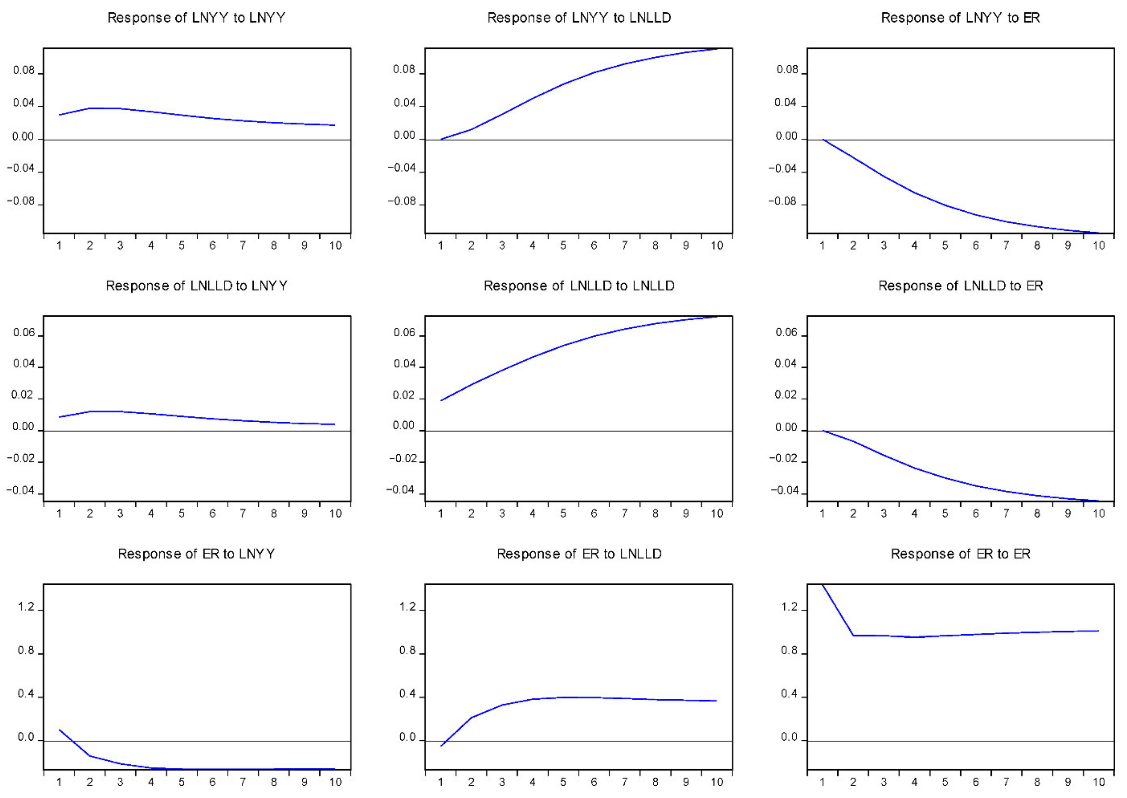
4.5. Contemporaneous Causality and Dynamic Relationship among Variables

The contemporaneous causal relationships between the series are represented in Figure 3. Each row illustrates the response of the same variable to the other variables, while each column reveals the response of the other variables to the same variable. The impulse reaction is measured in years. The first column demonstrates the effect of lnYY’s export on itself, lnLLD and ER. lnYY increased in response to itself for 10 years before levelling off over the course of the study period. ln LLDinitially rose in response to lnLYY before levelling off after 10 years. This suggests that processed seafood exports initially stimulated an increase in industrial upgrading and export performance investment. LnLYY has a negative effect on ER. This indicates that during the study period, processed exports have boosted industrial performance.

The second column demonstrates that lnLID positively affects itself, with the intensity peaking at 14 years and then levelling off. This suggests that industrial upgrading has a positive effect on itself over time. lnLLD also positively influences lnLYY, with lnLYY peaking after 18 years and then levelling off, indicating that investments in industrial upgrading over the past 18 years have increased exports of processed seafood. The third column demonstrates the influence of ER on itself, lnLYY and lnLID. ER had a negative impact on lnLYY and lnLLD. This indicates that exports of processed seafood are constrained by the current interaction between the exchange rate and investment in industrial upgrading.

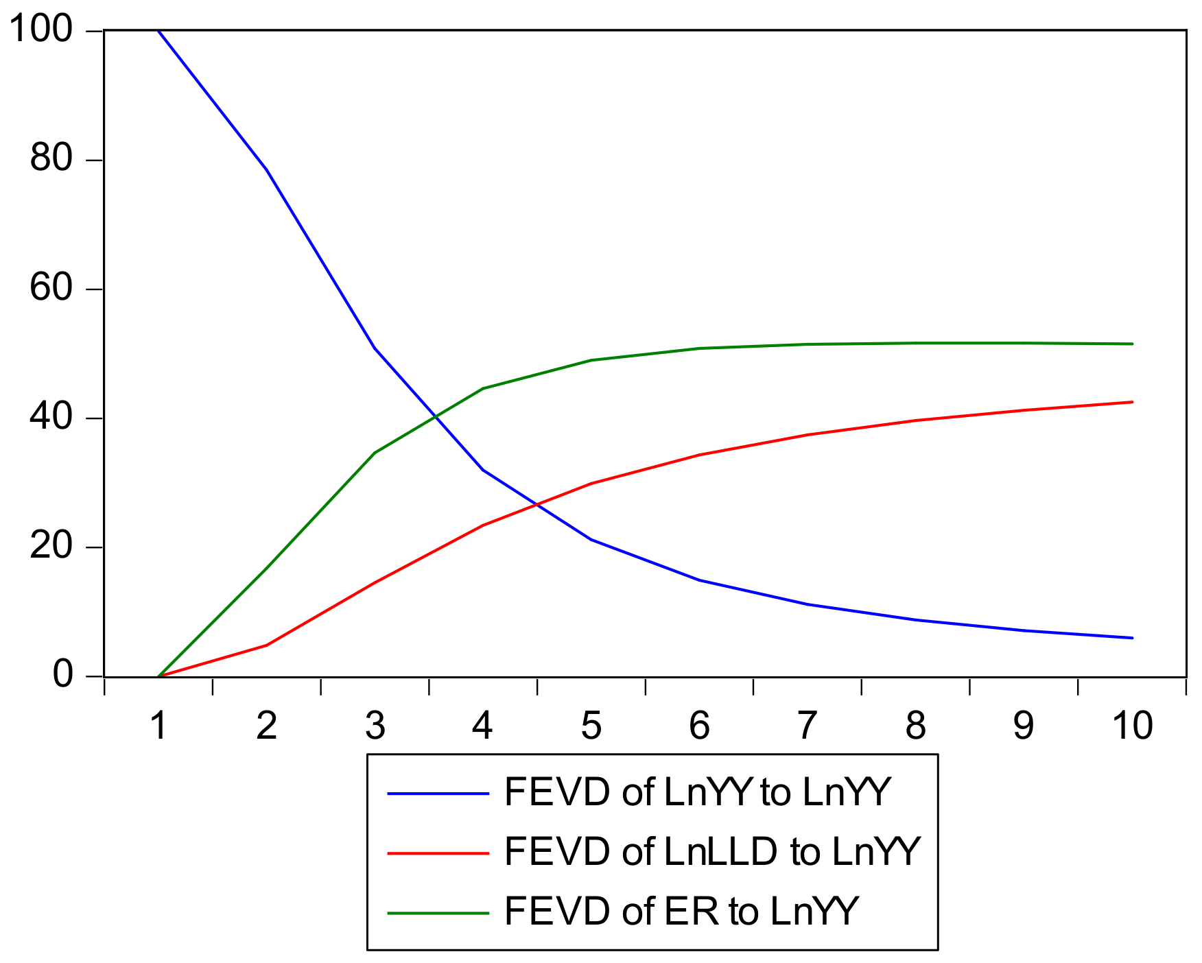
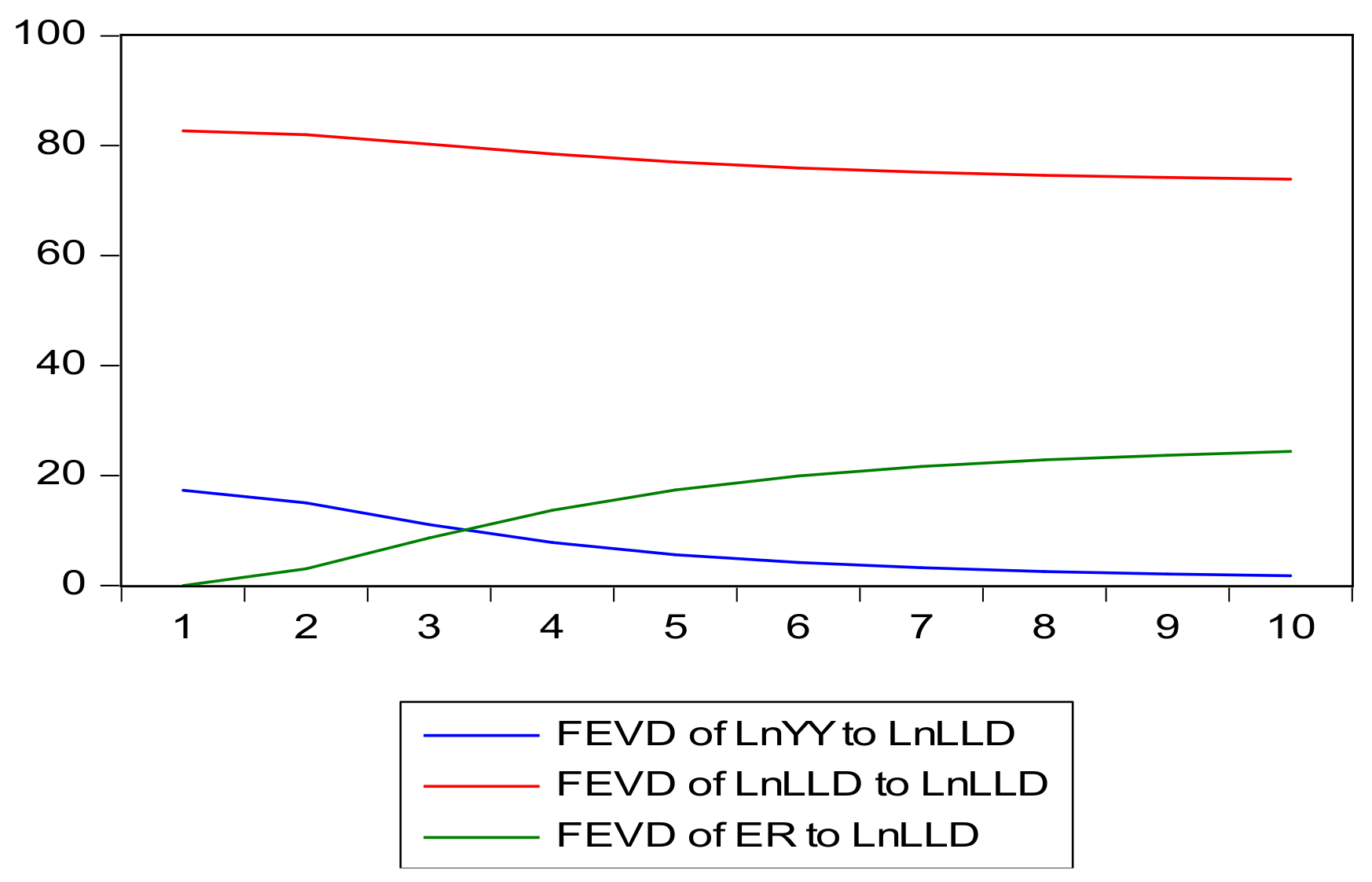
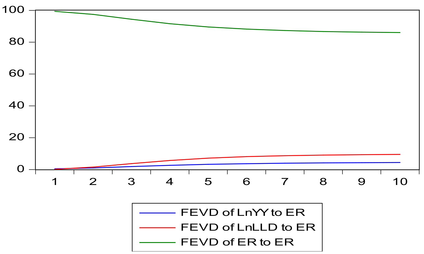
4.6. Variance Decomposition

The forecast error variance decomposition (FEVD) of lnYY is depicted in Figure 4. As depicted, the contribution of lnLLD and ER to the fluctuation variance of lnYY increased gradually over the course of the first eight periods before levelling off. In the initial period, lnYY had the greatest variance fluctuation, but this decreased over time, with ER contributing the most to the increase in variance. In Figure 5, the FEVD of ln LLD indicates that the contribution of ER was initially zero at period one before gradually increasing and stabilising after the 7th period, indicating that ER has a long-term effect on lnLLD. 73.8% of the fluctuations are attributable to lnLLD, so it would appear that lnLLD promotes industrial upgrading and export performance. Figure 6 indicates that ER itself explains a substantial proportion of FEVD. This explains the exchange rate’s autoregressive nature, whilst lnID and lnYY have little explanatory power.

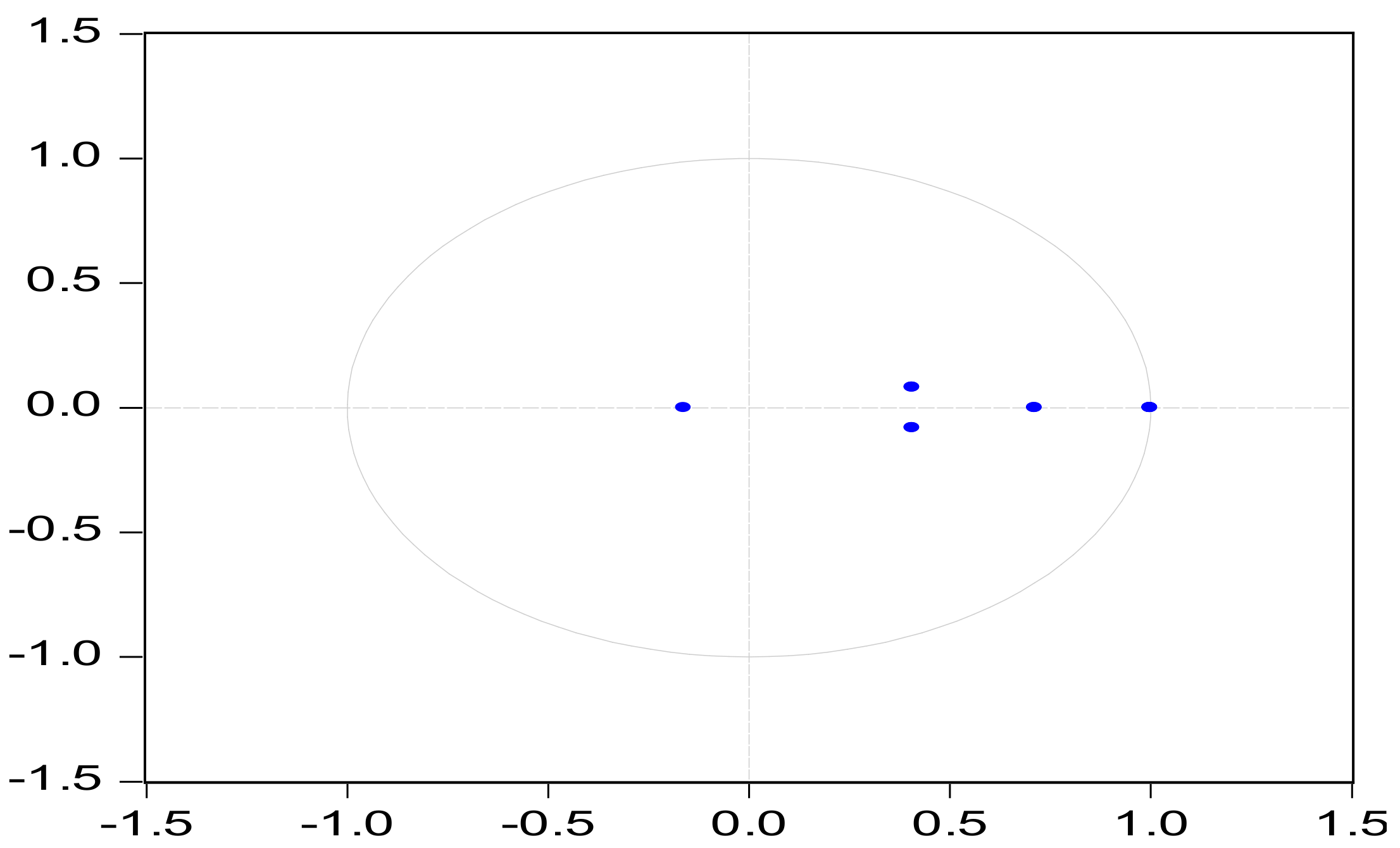
4.7. Robustness Checks

The results of the estimated VECM must exhibit a good relationship and establish the model’s predictability. Post diagnostics tests are conducted using the autocorrelation LM and heteroscedasticity tests.

From the results in

Table 8. Autocorrelation LM test results.

Lag	LMstatistic	Probability
1	8.927	0.445
2	16.920	0.170

Null hypothesis: No Serial Correlation.

and

Table 9. Heteroscedasticity tests results.

Chi-square Statistic	64.628
Prob.	0.0549

Null hypothesis: No heteroscedasticity.

, we fail to reject the null hypothesis of serial correlation and conclude there is no autocorrelation in the series. Furthermore, we reject the null hypothesis at 5%, indicating the model has no residual heteroscedasticity.

5. Discussion

Investment in industrial upgrading exhibits a long-run positive relationship with export, therefore, industrial upgrading of seafood processing facilities would enhance export quality and, consequently, export performance. This result supports the findings of Halpern [59] and Jouffray [60]. Empirical evidence from Section 4.4 shows that previous exchange rate short-run fluctuations affect industrial upgrading and exports. The underlying reason is that although currency depreciation limits the funds available for investment in industrial upgrading, currency depreciation enhances the amount of export flow. Therefore, taking advantage of currency depreciation is crucial to expand exports. From the VECM results, investment in industrial upgrading has a higher impact on exports than exchange rate, therefore, investment in industrial upgrading plays a significant role in mitigating the negative impact of exchange rate volatility. As a result, developing countries must improve industrial upgrading to sustain export performance.

Investment in industrial upgrading is self-promoting and enhances processed seafood exports. As most developing seafood exporting countries face financial constraints to long-term investment due to the high cost of capitalisation [50], private foreign partnerships could support industrial upgrading. After 20 years of reforms in the Namibian seafood industry, there still exists unprocessed exports of the two dominant export species; therefore, intervention from the private sector could change the structure of exports, consequently increasing export performance and economic growth. This is essential for achieving the vision 2030 vision [61].

6. Conclusions

This study investigated the causal relationships between industrial upgrading, exchange rate volatility and export performance of the Namibian seafood industry. As industrial upgrading and value addition are becoming increasingly important for the sustained export growth and economic development of seafood exporting developing countries, policymakers need to understand the dynamic relationship. In addition, the direction of causality provides a detailed understanding of the extent to which current exchange rate fluctuations affect exports in the long run and establishes a starting point for future efforts to increase investment in industrial upgrading.

The present study adds to the existing seafood export performance and exchange rate literature. It is the first study to incorporate industrial upgrading in the causation between export performance and exchange rate volatility. Using a VECM, variance decomposition and impulse response analysis, the results showed that investment in industrial upgrading is driven by both demand and supply factors. Additionally, this study provides evidence that industrial upgrading has a higher impact on exports than exchange rate fluctuations in the Namibian seafood industry. Therefore, investment in industrial upgrading plays a significant role in mitigating the negative impact of exchange rate volatility. While previous studies have mainly focused on how exchange rate might influence exports, this study includes investment expenditure in industrial upgrading to understand the dynamics.

In addition, the finding that the exchange rate in the previous period affects short-term fluctuations in industrial upgrading in the current period suggests that increased export volumes can mitigate future shocks to industrial upgrading. Therefore, the ability of seafood exporters to upgrade or add value to exports in response to future shocks will depend on their willingness to increase trade gains. Since Namibia’s investment in industrial upgrading is less than export growth, we recommend that the government improve supply-side policies to improve industrial upgrading. This study focused on Namibia’s seafood export performance as it relates to processed seafood exports. Even though processed seafood exports significantly impact Namibia’s economic growth, further analysis is required to achieve sustained economic growth from all other seafood export classifications. Future research should focus on how other products react to shocks associated with industrial upgrading.

References

1. Al-Busaidi, A.; David, J.J.; Shekar, B. Seafood Safety and Quality: An Analysis of the Supply Chain in the Sultanate of Oman. Food Control 2016, 59, 651–662. [Google Scholar] [CrossRef] [Green Version]
2. Bandara, T.; Abeywickrama, L.M.; Radampola, K. Growth Performance and Competitiveness of Finfish and Frozen Shrimp Exports in Sri Lanka. Indian J. Fish. 2020, 67, 118–126. [Google Scholar] [CrossRef]
3. Burhaz, M.; Soborova, O. Fisheries Development and the Formation of the Fish Products Market in Ukraine and in the Central and Eastern European Countries. Balt. J. Econ. Stud. 2020, 6, 10–18. [Google Scholar] [CrossRef]
4. Naabi, A.A.; Bose, S. Do Regulatory Measures Necessarily Affect Oman’s Seafood Export-Supply? SAGE Open 2020, 10. [Google Scholar] [CrossRef]
5. United Nations Conference on Trade and Development (UNCTAD). Fishery Exports and the Economic Development of Least Developed Countries 2017. United Nations, Gen. Available online: http://www.unctad.org/system/files/officialdocument/aldc2017d2_en.pdf (accessed on 27 March 2022).
6. Khasanah, M.; Nadiarti, N.; Yvonne, S.M.; Jamaluddin, J. Management of the Grouper Export Trade in Indonesia. Rev. Fish. Sci. Aquac. 2020, 28, 1–15. [Google Scholar] [CrossRef]
7. Carlucci, D.; Giuseppe, N.; Biagia, D.D.; Rosaria, V.; Francesco, B.; Gianluca, R. Consumer Purchasing Behaviour towards Fish and Seafood Products. Patterns and Insights from a Sample of International Studies. Appetite 2015, 84, 212–227. [Google Scholar] [CrossRef]
8. Macfadyen, G.; Ahmed, M.N.; Diaa, A.; Mohamed, F.; Hussien, H.; Ahmed, M.D.; Samy, M.H.; Ramadan, M.A.; Gamal, E. Value-Chain Analysis—An Assessment Methodology to Estimate Egyptian Aquaculture Sector Performance. Aquaculture 2012, 362, 18–27. [Google Scholar] [CrossRef]
9. Radhakrishnan, E.V.; Bruce, F.P.; Gopalakrishnan, A. Updated checklist of the world’s marine lobsters. In Lobsters: Biology, Fisheries and Aquaculture; Springer: Singapore, 2019; pp. 35–64. [Google Scholar]
10. Bennett, A.; Basurto, X.; Virdin, J.; Lin, X.; Betances, S.; Smith, M.; Allison, E.; Best, B.; Brownell, K. Recognise fish as food in policy discourse and development funding. Ambio 2021, 50, 981–989. [Google Scholar] [CrossRef]
11. Natale, F.; Alessandra, B.; Arina, M. Analysis of the Determinants of International Seafood Trade Using a Gravity Model. Mar. Policy 2015, 60, 98–106. [Google Scholar] [CrossRef]
12. Zhang, D.; Henry, W.K. Exchange Rate Volatility and US Import Demand for Salmon. Mar. Resour. Econ. 2014, 29, 411–430. [Google Scholar] [CrossRef]
13. Gianelli, I.; Omar, D. Uruguayan Fisheries under an Increasingly Globalised Scenario: Long-Term Landings and Bioeconomic Trends. Fish. Res. 2017, 190, 53–60. [Google Scholar] [CrossRef] [Green Version]
14. Goulart, P.; Francisco, J.V.; Catarina, G. The Evolution of Fisheries in Portugal: A Methodological Reappraisal with Insights from Economics. Fish. Res. 2018, 199, 76–80. [Google Scholar] [CrossRef]
15. Latief, R. The Effect of Exchange Rate Volatility on International Trade and Foreign Direct Investment (FDI) in Developing Countries along ‘One Belt and One Road’. Int. J. Financ. Stud. 2018, 6, 86. [Google Scholar] [CrossRef] [Green Version]
16. Monnaie, B.F. Upgrading and Allied Impacts on Contract Seafood Producers. OIDA J. Sustain. Dev. 2017, 2, 25–36. [Google Scholar]
17. Li, Q.; Li, Y. Economic marketing model of seafood in Beibu Gulf economic area. J. Coast. Res. 2020, 112, 248–251. [Google Scholar] [CrossRef]
18. Feng, S. Exchange Rate Flexibility of Marine Export Trade Based on Artificial Neural Network. J. Coast. Res. 2020, 104, 641–644. [Google Scholar] [CrossRef]
19. Asche, F.; Marc, F.B.; Cathy, R.; Martin, D.S.; Sigbjørn, T. Fair Enough? Food Security and the International Trade of Seafood. World Dev. 2015, 67, 151–160. [Google Scholar] [CrossRef]
20. Roheim, C.; Bush, S.; Asche, F.; Sanchirico, J.; Uchida, H. Evolution and future of the sustainable seafood market. Nat. Sustain. 2018, 8, 392–398. [Google Scholar] [CrossRef]
21. Straume, H.M. Currency Invoicing in Norwegian Salmon Export. Mar. Resour. Econ. 2014, 29, 391–409. [Google Scholar] [CrossRef] [Green Version]
22. Lee, M.; Mudziviri, N.; Sung, K.A. Transformation Strategy and Economic Performance: Hungary and Poland. East. Eur. Econ. 2014, 42, 25–42. [Google Scholar] [CrossRef]
23. Intarakumnerd, P.; Meng, L. Industrial Technology Upgrading and Innovation Policies: A Comparison of Taiwan and Thailand; Springer: Singapore, 2019. [Google Scholar]
24. Philippe, A.; Peter, H. A Model of Growth Through Creative Destruction. Econom. Soc. 1992, 60, 323–351. [Google Scholar]
25. Arrow, K.J. The Economic Implications of Learning by Doing. In Readings of the Theory of Growth; Macmillian Palgrave: London, UK, 1971; pp. 131–149. [Google Scholar]
26. Romer, P.M. Endogenous Technological Change. J. Political Econ. 1990, 98 Pt 2, S71–S102. [Google Scholar] [CrossRef] [Green Version]
27. Humphrey, J.; Hubert, S. How Does Insertion in Global Value Chains Affect Upgrading in Industrial Clusters? Reg. Stud. 2002, 36, 1017–1027. [Google Scholar] [CrossRef]
28. Ethier, W. International Trade and the Forward Exchange Market. Am. Econ. Rev. 1973, 63, 494–503. [Google Scholar]
29. Gagnon, E. Exchange Rate Variability International Trade. J. Int. Econ. 1993, 34, 269–287. [Google Scholar] [CrossRef] [Green Version]
30. Viaene, J.M.; De Vries, C.G. International Trade and Exchange Rate Volatility. Eur. Econ. Rev. 1992, 36, 1311–1321. [Google Scholar] [CrossRef] [Green Version]
31. Broll, U.; Eckwert, B. Exchange Rate Volatility and International Trade. South. Econ. J. 1999, 66, 178–185. [Google Scholar] [CrossRef] [Green Version]
32. Barkoulas, J.T.; Christopher, F.B. Exchange Rate Effects on the Volume and Variability of Trade Flows. J. Int. Money Financ. 2002, 21, 481–496. [Google Scholar] [CrossRef] [Green Version]
33. Aghion, P.; Bacchetta, P.; Ranciere, R.; Rogoff, K. Exchange Rate Volatility and Productivity Growth. The role of financial development. J. Monet. Econ. 2009, 56, 494–513. [Google Scholar] [CrossRef] [Green Version]
34. Grier, K.B.; Aaron, D.S. Uncertainty and Export Performance: Evidence from 18 countries. J. Money Credit. Bank. 2007, 39, 965–979. [Google Scholar] [CrossRef]
35. Bahmani, M.; Abera, G. Exchange-Rate Volatility and International Trade Performance: Evidence from 12 African Countries. Econ. Anal. Policy 2018, 58, 14–21. [Google Scholar] [CrossRef] [Green Version]
36. Intarakumnerd, P.; Pun, A.C.; Rungroge, K. Innovation System of the Seafood Industry in Thailand. Asian J. Technol. Innov. 2015, 23, 271–287. [Google Scholar] [CrossRef]
37. Fabinyi, M. Producing for Chinese Luxury Seafood Value Chains: Different Outcomes for Producers in the Philippines and North America. Mar. Policy 2016, 63, 184–190. [Google Scholar] [CrossRef]
38. Belton, B.; Thomas, R.; David, Z. Sustainable Commoditization of Seafood. Nat. Sustain. 2020, 3, 677–684. [Google Scholar] [CrossRef]
39. Wang, S.; Lu, B.; Yin, K. Financial Development, Productivity, and High-Quality Development of the Marine Economy. Mar. Policy 2021, 130, 104553. [Google Scholar] [CrossRef]
40. Péridy, N.; Patrice, G.; Pascal, B. The Impact of Prices on Seafood Trade: A Panel Data Analysis of the French Seafood Market. Mar. Resour. Econ. 2020, 15, 45–66. [Google Scholar] [CrossRef]
41. Nguyen, G.V.; Curtis, M.J. A Cointegration Analysis of Seafood Import Demand in Caribbean Countries. Appl. Econ. 2013, 45, 803–815. [Google Scholar] [CrossRef]
42. Marvasti, A.; David, W.C. Domestic and Imports Sources of Supply to the US Shrimp Market and Anti-Dumping Duties. J. Econ. Stud. 2016, 43, 1039–1056. [Google Scholar] [CrossRef]
43. Xie, J.; Henry, W.K.; Øystein, M. The Effects of Exchange Rates on Export Prices of Farmed Salmon. Mar. Resour. Econ. 2008, 23, 439–457. [Google Scholar] [CrossRef]
44. Zhang, D.; Ragnar, T. A Fish out of Water? Survival of Seafood Products from Developing Countries in the EU Market. Mar. Policy 2019, 103, 50–58. [Google Scholar] [CrossRef]
45. He, C.; Quagrainie, K.; Wang, H. Determinants of shrimp importation into the USA: An application of an augmented gravity model. J. Chin. Econ. Bus. Stud. 2013, 11, 219–228. [Google Scholar] [CrossRef]
46. Shao, Q.; Lijuan, C.; Ruoyu, Z.; Hongtao, W. Marine Economic growth, Technological Innovation, and Industrial Upgrading: A Vector Error Correction Model for China. Ocean. Coast. Manag. 2021, 200, 105481. [Google Scholar] [CrossRef]
47. Engle, R.F.; Granger, C.W.J. Co-Integration and Error Correction: Representation, Estimation, and Testing. Econom. Soc. 1987, 55, 251–276. [Google Scholar] [CrossRef]
48. Sims, C.A. Comparison of Interwar and Postwar Cycles: Monetarism Considered. Am. Econ. Rev. 1980, 70, 250–257. [Google Scholar]
49. Aghion, P.; Peter, H. Model of Growth through Creative Destruction. NBER Work. Pap. Ser. 1990, 3223, 1–50. [Google Scholar]
50. Sherbourne, R. A Guide to the Namibian Economy; Institute of Public Policy Research: Khomas, Namibia, 2017. [Google Scholar]
51. Johansen, S. Estimation and Hypothesis Testing of Cointegration Vectors in Gaussian Vector Autoregressive Models. Econometrica 1991, 59, 1551–1580. [Google Scholar] [CrossRef]
52. Bessler, D.A.; Yang, J.; Wongcharupan, M. Price Dynamics in the International Wheat Market: Modeling with Error Correction and Directed Acyclic Graphs. J. Reg. Sci. 2003, 43, 1–33. [Google Scholar] [CrossRef]
53. Seung, C.K. Estimating Dynamic Impacts of the Seafood Industry in Alaska. Mar. Resour. Econ. 2008, 23, 87–104. [Google Scholar] [CrossRef]
54. Phillips, P.C.B.; Pierre, P. Testing for a Unit Root in Time Series Regression. Biometrika 1988, 75, 335–346. [Google Scholar] [CrossRef]
55. Dickey, D.A.; Fuller, W.A. Likelihood Ratio Statistics for Autoregressive Time Series with a Unit Root. Econ. Soc. 1981, 46, 1057–1072. [Google Scholar] [CrossRef]
56. Kwiatkowski, D.; Phillips, P.C.; Schmidt, P.; Shin, Y. Testing the Null Hypothesis of Stationarity against the Alternative of a Unit Root How Sure Are We That Economic Time Series Have a Unit Root? J. Econ. 1992, 54, 159–178. [Google Scholar] [CrossRef]
57. Awokuse, T.O.; Joshua, M.D. The Causal Structure of Land Price Determinants. Can. J. Agric. Econ. 2006, 1303, 227–245. [Google Scholar] [CrossRef] [Green Version]
58. Zivot, E.; Andrews, D.W.K. Further evidence on the great crash, the oil-price shock, and the unit-root hypothesis. J. Bus. Econ. Stat. 2002, 20, 25–44. [Google Scholar] [CrossRef]
59. Johansen, S. Determination of cointegration rank in the presence of a linear trend. Oxf. Bull. Econ. Stat. 1992, 54, 383–397. [Google Scholar] [CrossRef]
60. Halpern, B.S. A Global Map of Human Impact on marine ecosystems. Science 2008, 319, 948–953. [Google Scholar] [CrossRef] [PubMed] [Green Version]
61. Ministry of Industrialisation, Trade and SMS Development (MITSMED). Strategic Plan 2017—2022. Republic of Namibia, Windhoek. 2017. Available online: https://www.mit.gov.na (accessed on 24 January 2022).
Figure 1. Namibia’s investment in industrial upgrading and processed seafood exports from 2008 to 2020. Author created.
Sustainability 14 07893 g001
Figure 2. Eigenvalues of the VECM.
Sustainability 14 07893 g002
Figure 3. Impulse response analysis.
Sustainability 14 07893 g003
Figure 4. Variance decomposition of LnYY.
Sustainability 14 07893 g004
Figure 5. Variance decomposition of LnLDD.
Sustainability 14 07893 g005
Figure 6. Variance decomposition of ER.
Sustainability 14 07893 g006