Abstract
The domestication of wild animals represents a major milestone for human civilization. Chicken is the largest domesticated livestock species and used for both eggs and meat. Chicken originate from the red junglefowl (Gallus gallus). Its adaptability to diverse environments and ease of selective breeding provides a unique genetic resource to address the challenges of food security in a world impacted by climatic change and human population growth. Habitat loss has caused population declines of red junglefowl in Thailand. However, genetic diversity is likely to remain in captive stocks. We determine the genetic diversity using microsatellite genotyping and the mitochondrial D-loop sequencing of wild red junglefowl. We identified potential distribution areas in Thailand using maximum entropy models. Protected areas in the central and upper southern regions of Thailand are highly suitable habitats. The Bayesian clustering analysis of the microsatellite markers revealed high genetic diversity in red junglefowl populations in Thailand. Our model predicted that forest ranges are a highly suitable habitat that has enabled the persistence of a large gene pool with a nationwide natural distribution. Understanding the red junglefowl allows us to implement improved resource management, species reintroduction, and sustainable development to support food security objectives for local people.
1. Introduction
The global population will reach 10 billion by 2050, spearheaded by economic growth in Southeast Asia [1]. Bioresources must be maximized through conservation and optimal food production while maintaining public health standards. Changes in land use, population growth, invasion by introduced species, bioresource overexploitation, and urbanization are critically endangering many ecosystems. Global biodiversity is declining, with many species facing extinction due to anthropogenic activities. By 2030, crop and pasture yields are likely to decline, leading to food insecurity [2]. Human food security requires producing sufficient quantities of both high-quality protein and dietary energy. The production of food crops grown on arable land can meet the human dietary energy demand. However, animal production more effectively meets high-quality protein requirements [3]. The economic costs of protein deficiencies are considerable, reducing the gross domestic product (GDP) by 2% in most developing countries, including Thailand [4]. Global losses in economic productivity due to protein deficiencies are higher than 2–3% of the GDP [4]. There are 12.3 million fewer people going hungry in Thailand than there were in 2009 (https://www.un.org/ecosoc/en/, accessed on 1 April 2022). Until recently, progress has been limited in local territories, where a difficult terrain and remote locations impact food security [5]. The ability of new crop combinations to provide high-quality protein is difficult for these people. Conversely, the potential of meeting their adequate daily dietary requirements (particularly using protein from animals) with an agroecological focus needs to be determined. These people have difficulty avoiding hunger and usually rely on intermediaries such as food pantries and soup kitchens. Therefore, food banks derived from natural ecological sources are very important and allow people to access their own food.
Thailand sits in the Indo-Burma biodiversity hotspot and exports agricultural products worldwide. Bioresources encompass over 10% of the land area, providing environmental support for a bio-circular and green (BCG) economy. The BCG economy is related to 17 of the global Sustainable Development Goals (SDGs) which are vital for future welfare and prosperity [6]. Chicken is one of the most ubiquitous domesticated animal bioresources, bred for both its eggs and meat as well as companion animals, ornamental birds, long-crowing birds, and game fighting birds [7,8,9,10,11,12,13]. Chickens residing in local communities are thought to have been domesticated approximately 8000 years ago from the red junglefowl (Gallus gallus, Linnaeus, 1758) [14]. The red jungle fowl is native to multiple regions, from Southeast Asia to Southwest China [15,16,17,18]. Red junglefowl are behaviorally different from domestic and indigenous chickens (such as Lueng-hang-khao, Pradu-hang-dam, and Betong), and are naturally very shy of humans. Compared to domestic and indigenous chickens, red junglefowl have a much smaller body mass and brighter coloration [19]. Domestic and indigenous chickens have acquired diverse genetic characteristics which have enabled them to adapt to new and challenging conditions in diverse locations by overcoming heat stress, humidity, and disease [18,20]. Over the last 100 years, commercial chicken breeds (including layers and broilers) have been selectively bred using various domestic and indigenous breeds [21,22,23,24]. However, the price of eggs and meat from domestic and indigenous chickens is generally higher than commercial layers and broilers because indigenous chickens are a secondary source of income for poultry farmers [25]. Conversely, in several local areas, the cost of domestic and indigenous chickens and their products are cheaper than the commercial varieties because indigenous chickens can represent a specific niche among the local people in remote highlands [26]. The promotion of local domestic and indigenous chicken farming has started in Thailand, especially in Chang Rai and Mae Hong Son [27]. Red junglefowls are a food bioresource which provides wild biodiversity and facilitates genetic diversity for domestic and indigenous chicken meat for locals [18].
Crossbreeding red junglefowl with domestic, indigenous, and commercial chickens has developed breeds that exhibit desirable traits [18]. However, the partial genetic admixture of the four chicken types requires repeated crossing which results in a reduction in genetic diversity, which can be observed through phenotypic morphology, while numbers of wild chickens are declining throughout the country [28]. Wild population decline has become a major concern for the Department of National Parks, Wildlife, and Plant Conservation (DNP), which promotes the wild biodiversity of red junglefowl. Recent research on the genetic diversity and population genetics of red junglefowl from wildlife research centers and indigenous chickens has revealed that some red junglefowl populations were not included in the ancestral populations of Thai indigenous chickens [18]. Red junglefowl in wildlife research centers are highly diverse due to their origins from populations in diverse geographical locations, suggesting a large available gene pool in Thailand [18]. In the different research centers, several individuals contained genetic heritage from 2 to 3 red junglefowl populations, suggesting genetic exchange or admixture across several centers and provinces. Therefore, it is critical to genetically conserve red junglefowl for biodiversity and food security.
A key issue in conservation biology is determining species distribution and extinction risk within the population range [29]. Understanding the distribution and abundance of a suitable habitat reduces ambiguity in the persistence of species occurring in large adjacent patches [30], and their potential dependence on environmental characteristics (such as climate) that provide important resources at crucial times [31,32,33]. Thus, investigating the relationships between red junglefowl and their preferred habitat enables us to predict the effects of habitat change, population management, and successful reintroduction [34]. Habitat suitability models predict the future potential distribution of wildlife [35,36]. Recently, maximum entropy has been incorporated into habitat suitability models (MaxEnt) [37]. Using this method, the coefficients of niche functions can be ecologically evaluated and converted into independent factors for interpretation [38]. We used MaxEnt to develop a pioneer model for red junglefowl resource management and reintroduction to mitigate biodiversity loss to restore and promote sustainable food security. MaxEnt uses ecological niche modeling to identify the potential distribution areas of red junglefowls in Thailand. We (1) identified the ecological best niche variables across the red junglefowl range and (2) mapped the potential distribution of red junglefowl. Red junglefowl genetic diversity and population gene pools from Chiang Mai Zoo (CMZ), Songkhla Zoo (SKZ), and Khon Kaen Zoo (KKZ) were recently independently derived from wild populations as the initial stage of a reintroduction program. The wild populations were examined as alternative resources to wildlife research centers. Our findings provide a guide for a conservation program to support and maintain biodiversity and bioresources for food security.
2. Materials and Methods
2.1. Input Data
The modeling incorporated the entire mainland and islands of Thailand. The habitat suitability model for red junglefowl (G. gallus, including G. gallus gallus, and G. gallus spadiceus) used data from an area encompassing 513,000 km2 (5–16° N, 97–105° E). The red junglefowl observation locations within Thailand were obtained from the eBird Basic Dataset [39]. From 2015 to 2020, 560 red junglefowl observations were recorded (Table S1). After condensing the data into square kilometer grid cells, 519 grid locations constructed the habitat suitability model. We combined the data with three independent environmental datasets (elevation, forest canopy height, and climate data) to build a habitat suitability model (Table S2). Elevation data were obtained from the United States Geological Survey (USGS) database. The forest canopy height data were sourced from the Global Ecosystem Dynamics Investigation (GEDI) [40]. Global bioclimatic variables were retrieved from the WorldClim2 dataset [41] representing current climates (averaged for the period 1950–2000). Climate estimates for two future time periods, namely 2050 and 2070, were applied as transfer layers. The future scenario layers used the representative concentration pathway (RCP) 4.5 emission scenario using CMIP5 general circulation models (MPI-ESM-LR) with the known performance and suitability model data from across the regions of Southeast Asia [42]. We excluded four data layers that contained artifactual values expressing abrupt or unrealistic climatic changes between neighboring pixels (i.e., 8, 9, 18, and 19). All environmental datasets had the same spatial resolution (approximately 1 km2) in GeoTiff format to predict the distribution of red junglefowl in Thailand [43].
2.2. Species Distribution Modeling
The maximum entropy (MaxEnt) algorithm built the red junglefowl distribution model (MaxEnt) [37] using MaxEnt 3.4.1 software [44]. This machine-learning algorithm predicted species potential distributions by combining the environmental predictors and location data [45]. When the location area was very small, MaxEnt only used the location-only data to predict the species distribution [46,47,48]. We selected the logistic output with suitability values ranging from 0 to 1, which represent the occurrence probability of the target species, with the default settings for the convergence threshold and maximum number of iterations (500) [49]. Regularization values were automatically selected by the MaxEnt software to reduce over-fitting the model [48,50]. The robustness of each model was examined by cross-validation with five replicates, i.e., 20% of presence locations were used as the test data for each replicate [51]. The entire red junglefowl location data were split into training data (80%) and testing data (20%) in each replicate. To decrease the predictive uncertainty, we used the ensemble forecasting approach as previously described by Araújo and New [52]. We also applied the basic mathematical function of mean ensembles to calculate the final logistic outputs [53]. Model validation and predictive performance evaluated the area under the curve (AUC) of the receiver operating characteristics (ROC) [54]. The AUC values were threshold-independent measures of model accuracy to illustrate the model’s discrimination ability [54]. In this model, an AUC value of 0 indicated a model with no better discrimination than chance, an AUC value of 1 indicated perfect discrimination, and an AUC value > 0.8 indicated excellent discrimination.
2.3. Climate Change Threats
To compare future scenarios, we projected species distributions in the current climate, 2050, and 2070. We also overlaid the boundaries of the protected areas (PAs). The PAs are intensive study areas that are available from the Department of National Parks, Wildlife, and Plant Conservation. These data provide a suitable habitat for wild chickens inside and outside PAs (Table S3).
2.4. Specimen Collection and DNA Extraction
Fifty red junglefowls were sampled from Chiang Mai Zoo (CMZ) and had derived from Mae Hong Son (19°18′04″ N, 98°56′48″ E) and Chiang Rai Zoo (10°56′30″ N, 100°17′41″ E), Songkhla Zoo (SKZ) derived from Surat Thani (9°09′04″ N, 99°17′41″ E) and Satun (7°38′37″ N, 100°05′48″ E), and Khon Kaen Zoo (KKZ) derived from Phu Phan (17°04′23″ N, 104°59′48″ E), and Sakon Nakhon (17°04′23″ N, 104°10′32″ E). The red junglefowls were residents in the three zoos. Red junglefowl subspecies were distinguished by morphological traits: G. gallus gallus have red earlobes, whereas G. gallus spadiceus have white earlobes [55,56]. Detailed information on the sampled populations is provided in Table S4. Blood was sampled from the wing veins of live chickens using a Vacuette® 21-gauge needles and stored in vials containing 5 mM EDTA (Greiner Bio-One, Kremsmünster, Austria) at 25 °C until required for analysis. Whole genomic DNA was extracted following the standard salting-out protocol, as previously described in Supikamolseni et al. [57] and used as PCR templates. DNA quality and concentration were determined using 1% agarose gel electrophoresis and a NanoDrop™ 2000 Spectrophotometer (Thermo Fisher Scientific, Wilmington, DE, USA). The experimental design was approved by the Zoological Park Organization of Thailand (ZPO), Ministry of Natural Resources and Environment. Animal care and all experimental procedures were approved by the Animal Experiment Committee in ZPO, following the annual physical examination protocol and the Animal Experiment Committee of Kasetsart University (ACKU65-SCI-017) and conducted in accordance with the Regulations on Animal Experiments at Kasetsart University.
2.5. Mitochondrial D-Loop Sequencing
The mitochondrial D-loop (mt D-loop) fragments were amplified by PCR using the primers: Gg_D-loop_1F (5′-AGGACTACGGCTTGAAAAGC-3′) and Gg_D-loop_4R (5′-CGCAACGCAGGTGTAGTC-3′) [18,54,58]. Each PCR amplification used 15 μL of 1 × ThermoPol® buffer that contained 1.5 mM MgCl2, 0.2 mM dNTPs, 5.0 μM primers, 0.5 U Taq polymerase (Apsalagen Co., Ltd., Bangkok, Thailand) and 25 ng genomic DNA. The PCR conditions were as follows: initial denaturation at 95 °C for 30 min, followed by 35 cycles at 95 °C for 30 s, 58 °C for 30 s, 72 °C for 30 s, and finally an extension for 5 min at 72 °C. The PCR products were detected by electrophoresis in 1% agarose gel. The PCR products were purified using the GenUP™ PCR Cleanup Kit (Biotechrabbit, Hennigsdorf, Germany) following the manufacturer’s instructions. Nucleotide sequences of the DNA fragments were determined by the DNA sequencing service of First Base Laboratories Sdn Bhd (Seri Kembangan, Selangor, Malaysia). The BLASTn and BLASTx programs (http://blast.ncbi.nlm.nih.gov/Blast.cgi, accessed on 20 May 2022) searched the nucleotide sequences in the National Center for the Biotechnology Information database to confirm the identity of the amplified DNA fragments. The resulting sequences were deposited in the DNA Data Bank of Japan (DDBJ) (https://www.ddbj.nig.ac.jp/, accessed on 20 May 2022) (accession number: LC710555–LC710596) (Table S4).
2.6. Mitochondrial D-Loop Sequence Analysis
Multiple sequence alignments were performed for 446 (42 + 404) sequences in the mt D-loop dataset, including 404 (125 indigenous chicken breeds and 279 red junglefowls) chicken sequences retrieved from the reference dataset from our previous research [18]. The sequences were aligned using the default parameters of the Molecular Evolutionary Genetics Analysis 11 (MEGA11) software [59]. All unalignable and any sites containing gaps were carefully removed and trimmed from the datasets. Ambiguous sites behind the primer sequences were trimmed from the fragments. Estimates of the haplotype (h) and nucleotide (π) diversity [60], number of haplotypes (H), the estimator theta (S), overall haplotype, and average number of nucleotide differences (k) were calculated using the mt D-loop sequences of each zoo population using DnaSP version 6.12.03 [61]. A statistical parsimony network of the consensus sequences was constructed using the Templeton, Crandall, and Sing (TCS) algorithm in PopART version 1.7 to examine the haplotype grouping and population dynamics [62]. DNA sequences were aligned using the Geneious Alignment method in Geneious Prime (version 2022.0.2) (http://www.geneious.com, accessed on 20 May 2022) [63]. To determine the phylogenetic positions and haplogroup of the red junglefowls from the zoos, the phylogenetic analysis was performed using a Bayesian inference with MrBayes version 3.2.6 [64]. The best-fit model of DNA substitution was determined for each genetic region using Kakusan4 [65]. The MCMC process ran four chains simultaneously for one million generations. After stabilizing the log-likelihood value, a sampling procedure was performed every 100 generations to obtain 10,000 trees and generate a majority-rule consensus tree with mean branch lengths. All initial sample points were discarded as the burn-in period. The Bayesian posterior probability of the sampled tree population was calculated as a percentage. The genetic differentiation coefficient (GST), Wright’s F-statistic for subpopulations within the total population (FST), and the ΦST values from the sequence data and haplotype data were estimated using Arlequin version 3.5.2.2 [66]. The FST and ΦST values were calculated by analyzing 1000 permutations of haplotypes between the populations [67]. The FST statistic relied on the differences in the haplotype frequencies, whereas ΦST considers the relationship between the haplotypes based on molecular genetic distance [68]. The average number of nucleotide substitutions for each site between populations (Dxy) and the net nucleotide substitutions of each site between populations (Da) were analyzed using DnaSP version 6.12.03 [61].
2.7. Genotyping of Microsatellite Markers
Twenty-eight microsatellite primer sets were selected from the 30 markers recommended for chicken biodiversity studies by the Food and Agriculture Organization [69] (Table S5). The 5′-end of the forward primer of each primer set was labeled with fluorescent dye (6-FAM or HEX; Macrogen Inc., Seoul, Korea). PCR amplification used 15 μL of 1× ThermoPol buffer containing 1.5 mM MgCl2, 0.2 mM dNTPs, 5.0 μM primers, 0.5 U Taq polymerase (Apsalagen Co., Ltd., Bangkok, Thailand), and 25 ng genomic DNA. The PCR protocol was as follows: initial denaturation at 94 °C for 3 min, followed by 35 cycles at 94 °C for 30 s, 52–61 °C for 30 s, and 72 °C for 30 s, with a final extension at 72 °C for 10 min (Table S5). The PCR products were detected by electrophoresis in 1% agarose gel. A minimum of three PCR amplifications were performed on each sample to reduce the influence of false alleles. PCR product absences were examined using 1% agarose gel electrophoresis. A fluorescent DNA fragment length analysis was performed using an ABI 3730XL automatic sequencer (Applied Biosystems, Foster City, CA, USA) at the DNA sequencing service of Macrogen Inc. Allelic size was determined using the Peak Scanner version 1.0 software (Applied Biosystems). The genotypic data can be accessed from the Dryad Digital Repository Dataset, https://doi.org/10.1038/s41598-021-81589-7, accessed on 20 May 2022.
2.8. Analysis of Genetic Diversity using Microsatellite DNA Markers
The microsatellite DNA analysis followed the same procedure outlined in our previous animal research projects [70,71,72,73,74]. The allelic frequency, number of alleles (A), effective number of alleles (Na), observed heterozygosity (Ho), expected heterozygosity (He), linkage equilibrium, and Wright’s F-statistic for subpopulations within the total population (FST) were calculated using Arlequin version 3.5.2.2 [66]. Due to limited population sizes, the deviations from the Hardy–Weinberg equilibrium were evaluated at each locus by the Markov chain Monte Carlo (MCMC) approximation of Fisher’s exact test using the “genepop” function in the package “stats” of R version 4.1.2 [75,76,77]. Welch’s t-test (unequal variance between samples) identified any significant differences between Ho and He using the “t.test” function in “stats” of R version 4.1.2 [77,78]. To test for equal variances between the Ho and He, Bartlett’s homogeneity of variance test was performed using the “bartlett.test” function in “stats” of R version 4.1.2 [77]. Allelic richness (AR) was calculated by FSTAT version 2.9.4 [79]. MicroChecker version 2.2.3 identified the null allelic markers [80]. The polymorphic information content (PIC) was estimated using the Excel Microsatellite Toolkit [81] and calculated for each locus. Shannon’s information index (I) and the fixation index (F) were calculated for each locus of the population using GenAlEx version 6.5 [82]. The effective population size (Ne) was estimated as the number of breeding individuals that contributed to the population using the linkage disequilibrium method in NeEstimator version 2.01 [83].
Individual and overall FIS (with 95% confidence intervals) were calculated using the LynchRt estimator [84] of COANCESTRY [85]. FIS was examined using the assumption that the averages did not significantly differ from randomly selected unrelated individuals. The distribution of the pairwise FIS values between all zoo pairs (samples collected from the zoos) were compared using a bootstrap version of the Kolmogorov–Smirnov test to identify relationships [86] using the “ks.test” function in “stats” of R version 4.1.2 [77]. To evaluate the group structure, an analysis of molecular variance (AMOVA) was performed using Arlequin 3.5.2.2. Unlike FST, this algorithm identifies the subgroup hierarchical structures and does not depend on the Hardy–Weinberg equilibrium.
The model-based clustering method in STRUCTURE version 2.3.4 determined the population structure [87]. The run length was set at 100,000 MCMC replicates after a burn-in period of 100,000 generations and used correlated allelic frequencies of a straight admixture model. The number of clusters (K) varied from 1 to 25, with 25 replicates for each value of K. The most probable number of bunches was identified by plotting the log likelihood of the information (ln Pr (X|K)) [87] over the scope of the K esteems before choosing the K esteem value at which ln Pr (X|K) settled. The ΔK strategy was applied utilizing Structure Harvester [88].
3. Results
3.1. Modeling Evaluation
The AUC values were 0.8, suggesting that the SDMs performed well for red junglefowls. A cross-validation revealed that the models were robust, with relatively high accuracy in both the training and testing data. The variables providing the greatest average contribution to the MaxEnt model were (i) forest canopy height (15.6% of mean contribution); (ii) maximum temperature of the warmest month (BIO5; 14.9%); (iii) annual precipitation (BIO12; 13%); (iv) temperature annual range (BIO7; 8.7%); (v) temperature seasonality (BIO4; 7.9%); and (vi) precipitation seasonality (BIO15; 7.5%), which summarized the 11 variables (32.6%) (Figure 1, Table S6).
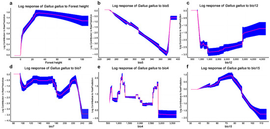
Figure 1.
MaxEnt model response area curves influencing wild red junglefowl distributions with predictor variables: forest canopy height (a), maximum temperature of the warmest month (BIO5) (b), annual precipitation (BIO12) (c), annual temperature range (BIO7) (d), temperature seasonality (BIO4) (e), and precipitation seasonality (BIO15) (f).
3.2. Habitat Suitability
The current climate-based potential geographic distribution of red junglefowls revealed that their range was almost entirely restricted to upper southern and central Thailand, with only a few patches of suitable habitat in the north and west. The PAs in central and upper southern Thailand are highly suitable for red junglefowls. Highly suitable areas were also located outside PAs in the upper southern and western areas. Future projections of 2050 and 2070 showed the red junglefowl distribution expanding with increased habitat suitability due to the combined effects of future climate forest canopy height and elevation. The results for both 2050 and 2070 showed a range expansion with high suitability (Table S3). Most expansions occurred in the upper southern, central, and western areas. Central and upper southern areas increased in suitability, both outside and inside the PAs (Figure 2).
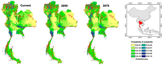
Figure 2.
Suitable habitat for red junglefowl under current and future climate change scenarios at two time scales projected for Thailand in 2050 and 2070.
3.3. Genetic Variability of Red Junglefowl Populations in Captivity Based on Mitochondrial Haplotype Analysis
The amplicon length was 1200 bp and the alignment length was 732 bp in the mt D-loop sequences with 19 haplotypes. The overall haplotype and nucleotide diversities were 0.936 ± 0.020 and 0.023 ± 0.012 in the mt D-loop sequences (Table 1), respectively. A complex haplotype network was constructed using the large number of detected polymorphic sites and haplotypes (Figure 3). The most common haplotype in all populations was CK16 which belonged to haplogroup B. Ten haplotypes (CK2, CK4, CK6, CK7, CK8, CK10, CK12, CK14, CK15, and CK16) belonging to haplogroups A, B, CD, and J were shared among the CMZ, SKZ1 (G. gallus gallus), SKZ2 (G. gallus spadiceus), and KKZ populations. Following Hata et al. [18], we treated haplogroups C and D as one unit (CD) as they did not clearly separate. To examine genetic differentiation among the four populations, we calculated FST, GST, ΦST, Dxy, and Da. The FST ranged from −0.076 to 0.308, the GST ranged from 0.030 to 0.095, and the ΦST ranged from 0.039 to 0.175 for the mt D-loop sequences (Table 2). The Dxy ranged from 0.010 to 0.017 and the Da ranged from −0.001 to 0.005 for the mt D-loop sequences (Table 2).

Table 1.
Mitochondrial D-loop sequence diversity for red junglefowls (Gallus gallus, Linnaeus, 1758) [14] in Thailand.

Figure 3.
Haplotype network based on the mitochondrial D-loop region sequence data of red junglefowls (Gallus gallus, Linnaeus, 1758) [14] from Chiang Mai Zoo (haplotype CK7, CK9, CK15, CK18, and CK19), Songkhla Zoo (haplotype CK1, CK6, CK8, CK10, CK12, CK13, and CK14), and Khon Kaen Zoo (haplotype CK2, CK3, CK4, CK15, CK16, and CK17).
Table 2.
Genetic differentiation between the four red junglefowl populations (Gallus gallus, Linnaeus, 1758) [14] using D-loop sequences. Genetic differentiation coefficient (GST), Wright’s F-statistics for subpopulations within the total population (FST), ΦST from sequence data and haplotype data, the average number of nucleotide substitutions per site between populations (Dxy), and the net nucleotide substitutions per site between populations (Da).
3.4. Genetic Variability of Red Junglefowls in Captivity Based on Microsatellite Data
All captive individual red junglefowls were genotyped with 326 alleles observed among all loci, and the mean number of alleles per locus was 9.527 ± 0.469 (Table 3). All allelic frequencies had significantly departed from the Hardy–Weinberg equilibrium of the captive population, with multiple lines of evidence for linkage disequilibrium (Tables S7–S10). Null alleles were frequently identified for twenty-eight loci (Table S5), and all markers were treated similarly. The SKZ1 and SKZ2 populations exhibited negative F-values that were positive in the CMZ and KKZ populations. The PIC of all populations ranged from 0.195 to 0.868 and I-values ranged from 0.000 to 2.164 (Table S11). The Ho values ranged from 0.000 to 1.000 (mean ± standard error (SE): 0.626 ± 0.026) and the He values ranged from 0.000 to 0.880 (mean ± SE: 0.678 ± 0.014) (Table 3, Table S11). Welch’s t-test revealed that the Ho was significantly different from He in the KKZ population, 19 individuals (Ho = 0.401 ± 0.061, He = 0.682 ± 0.032, t = −4.079, and df = −0.281, p < 0.05), but not significantly different in the CMZ population, 7 individuals (Ho = 0.671 ± 0.040, He = 0.692 ± 0.024, t = −0.450, df = −0.021, p = 0.662), the SKZ1 population, 12 individuals (Ho = 0.678 ± 0.038, He = 0.672 ± 0.031, t = 0.122, df = 0.006, p = 0.904), or the SKZ2 population, 4 individuals (Ho = 0.756 ± 0.040, He = 0.666 ± 0.026, t = 1.886, df = 0.090, p = 0.116). The pairwise Ho values between the populations were not statistically different between CMZ and SKZ1. Conversely, all pairwise He values between the populations were not statistically different (Table S12). The AR value of the population was 9.527 ± 0.469. The standard genetic diversity indices are summarized in Table 3 and Table S11.
Table 3.
Genetic diversity among 42 red junglefowls (Gallus gallus, Linnaeus, 1758) [14] based on 28 microsatellite loci.
The mean FIS was 0.001 ± 0.045 (Table 4), with individual values of FIS ranging from −0.093 to 0.350 (Table S13). However, the FIS distributions of the CMZ, SKZ1, SKZ2, and KKZ populations varied significantly (Figure S1, Table S14). The Ne for individuals from the CMZ population was 22.300 (95% CI: 12.500–63.700), the Ne for the SKZ1 population was 7.200 (95% CI: 5.500–9.200), and the Ne for the KKZ population was 43.300 (95% CI: 29.000–79.200) (Table 4). AMOVA revealed that the genetic variation was 24% among individuals within a population with 14% variation between populations (Table S15).
Table 4.
Inbreeding coefficients, relatedness, effective population size, and the ratio of effective population size with the census population (Ne/n) of Asian chickens (Gallus gallus, Linnaeus, 1758) [14] at the Chiang Mai Zoo, Songkhla Zoo, and Khon Kaen Zoo.
The gene pool groups of the red junglefowls were compared with the reference baseline data from our previous study [18]. The model-based Bayesian clustering algorithms of STRUCTURE generated different population patterns with increasing K-values from 2, 3, 4, 5, 10, and 20, based on individual chicken samples from this study and the populations in Hata et al. [18]. The optimized population structure patterns were assigned into three clusters (K = 20) using Evanno’s ΔK (Figure 4). Multiple gene pool clusters were observed in the CMZ, SKZ1, and SKZ2 populations.
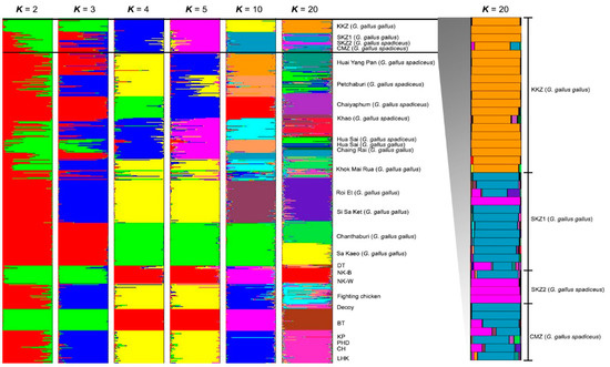
Figure 4.
Population structure of 42 red junglefowls (Gallus, Linnaeus, 1758) [14]. Each vertical bar on the x axis represents an individual, while the y axis represents the membership proportions (posterior probability) in each genetic cluster. Red junglefowls are superimposed on the plot with boundaries depicted by black vertical lines. Detailed information on all of the individual red junglefowls is presented in Supplementary Table S4. KKZ = Khon Kaen Zoo; SKZ1 = Songkhla Zoo (G. gallus gallus); SKZ2 = Songkhla Zoo (G. gallus spadiceus); CMZ = Chiang Mai Zoo; DT = Dong-Tao; NK-B = Nin Kaset meat chicken with black feathers; NK-W = Nin Kaset meat chicken with white feathers; BT = Betong; KP = Kheaw-Paree; PHD = Pradu-hang-dam; CH = Chee; LHK = Lueng-hang-khao.
4. Discussion
Given the threats facing declining red junglefowl populations in Thailand [18], mitigation by resource management and reintroduction is necessary to recover their abundance and provide food security through long-term sustainable management. In addition to the genetic gene pool analysis for reintroduction management, we designed the habitat suitability spatial models to ensure science-based decisions for successful red junglefowl conservation in target areas.
4.1. Habitat for Long-Term Red Junglefowl Reintroduction
Climate change may instigate an increase in suitable habitat for red junglefowl due to the combined effects of climate elevation and forest canopy height. Canopy height acts as an effective surrogate of woodland structure and can be applied as a predictor of woodland bird composition and distribution [89]. Our distribution model revealed a strong positive relationship between red junglefowl distribution and forest canopy height and a limited relationship with climate and elevation (Figure 1 and Table S3). Suitable red junglefowl habitats should increase in landscapes as they progress towards higher vegetation diversity, i.e., the succession to more complex habitats from shrubland or grassland systems [90]. Red junglefowl distributions will also shift westward and upward in the climate change scenarios (Figure 2). Current highly suitable areas (suitability > 0.8) for red junglefowl encompass 8569 km2 (inside PAs 4802 km2 and outside PAs 3767 km2). The PAs provide highly suitable habitats for red junglefowl throughout their distribution range. Highly suitable areas are predicted to increase to 10,001 km2 and 9466 km2 in the 2050 and 2070 scenarios, respectively. Future scenarios are similar to current conditions with one exception. The suitable areas will expand inside the PAs in Kaeng Krachan National Park (12°60′31″ N, 99°37′37″ E), Khao Yai National Park (12°60′31″ N, 101°22′19″ E), Mae Paem National Park (19°21′14″ N, 99°52′31″ E), Huay Nam Dang National Park (19°18′14″ N, 98°35′56″ E), Doi Inthanon National Park (19°35′28″ N, 98°29′13″ E), and Umphang Wildlife Sanctuary (15°57′56″ N, 98°46′08″ E). In the future, red junglefowl distribution will mainly be affected by changing climatic conditions altering future land uses. In future scenarios, western areas possess high and medium suitability for red junglefowls.
4.2. Reintroduction of Red Junglefowl with Large Gene Pool Variations
The four zoo populations presented high genetic variability, similar to the red junglefowl specimens from wildlife research centers in Thailand [18]. We investigated the zoo gene pool with the wild genetic resources by assessing all genetic characteristics derived from microsatellite and mt D-loop data. Our study results were compared with those of our previous research on red junglefowl from wildlife conservation centers [18]. The genetic characteristics of the microsatellite data showed the KKZ population clustered with the zoo populations [18], whereas the KKZ population haplogroups were derived from B and J. Haplogroups A–E and J were likely to be the common haplogroups in Thai red junglefowl, in contrast to other rare haplogroups, which were identified in many Asian regions (Haplogroup G in China, Sri Lanka, Laos, and Vietnam; haplogroup I in India; haplogroup K in Indonesia; and haplogroups W–Z in China) [17,18]. These results collectively suggest that the red junglefowl populations in Thailand possess large gene pools with extensive genetic diversity which have been conserved in several populations for a long time. The CMZ population shared genes with the Chiang Rai Wildlife Conservation Center, and both were consistent with haplogroup J. This might result from geographically adjacent original sources in Northern Thailand. By contrast, the SKZ population were in multiple gene pool clusters. The SKZ1 population shared a gene pool with Chiang Rai, despite the large geographical distance from the original source. The SKZ2 population shared a gene pool with the CMZ population. At least three of the four populations collected from the wild showed mixed gene pools among geographically different regions with the reference baseline [18]. This result was consistent for both the microsatellite genotyping and mitochondrial D-loop sequencing. Similar cases were observed in Huai Sai and Petchaburi Wildlife Conservation Centers. Red junglefowls cannot fly and move over a home range of approximately 5 ha. The habitat sampling area was selected as 1 km2 [91]. There may be genetic exchange between the wildlife conservation centers across different provinces [18].
Red junglefowl individuals in each wildlife center were consistently derived from local wild populations [35]. This leads us to propose the alternative explanation of a very large gene pool existing in several wild populations in Thailand. Kaeng Krachan National Park (12°60′31″ N, 99°37′37″ E) showed excellent habitat suitability and fit with the ecological landscape for red junglefowl distribution and population expansion, while the Huai Sai and Petchaburi Wildlife Research Centers contained multiple clusters of gene pools [18]. Kaeng Krachan National Park, Huai Sai, and Petchaburi Wildlife Research Centers are located in the same forest range. Therefore, the gene pool of the original source populations of CMZ and SKZ were partially shared due to the wide home range of these large gene pools. However, range expansion within the same gene pool was probably aided by intentional human introduction via domestic or wild red junglefowls. Moreover, within Huai Sai and Petchaburi Wildlife Research Centers, red junglefowl populations contained haplogroups A and B, which were also observed in the CMZ population. The high habitat suitability of Kaeng Krachan National Park might influence the existence of a large gene pool with a large distribution range across the country. No specific gene pools and haplogroups were found between G. gallus spadiceus and G. gallus gallus in the red junglefowl populations of Huai Sai and Petchaburi Wildlife Research Centers [18]. A similar case was also observed in red junglefowls in this study, reflecting the occurrence of gene flow between different subspecies. In contrast, this might suggest the existence of two subspecies, differentiated by earlobe color [55]. Various earlobe colors from red to white (or partial white) are observed in red junglefowl and domestic chickens [55]. Revision of the species and subspecies levels in chicken is probably needed to clarify these taxonomic discrepancies. Variations in chicken earlobe colors might be the result of dimorphism, derived from phenotypic and ecological divergence within the species [92]. Population-level assessments of red junglefowl are required to facilitate the maintenance and preservation of their genetic diversity and their characteristics in different conservation centers or provinces. These genomic changes must corroborate whole-genome studies to analyze the distribution of SNPs in red junglefowls. Currently, there is no specific understanding of the dispersal processes of red junglefowls due to the absence of studies using high-resolution genetic markers. By analyzing SNPs in large regions of the genome or complete genomes, robust results can be obtained for gene flow and genetic differentiation dispersion processes [93].
4.3. Food Bank and Food Security in Relation to SDGs
Global food and nutritional security relies on national or regional areas addressing their own food needs. Future food availability and nutritional security have become major concerns for both the rich and poor, given the present concurrence of rising human population, global warming, and changing consumption habits [94]. To feed the world in 2050, we need to increase total global food production by 70% [2]. This is increasingly challenging in a changing climate. Meanwhile, traditional local and indigenous cultures maintain free-range domestic and indigenous chickens that potentially interbreed with red junglefowls. Dominant males attempt to maintain exclusive reproductive access to females. However, approximately 40% of mating involves subordinate males in a free-ranging feral flock. Therefore, the red junglefowl is a very important genetic resource for improving the gene pool of domestic and indigenous chickens. The reintroduction of red junglefowl into the wild will improve the genetic diversity of red junglefowls. We suggest that a red junglefowl reintroduction plan for the most efficient food security should focus on the release of red junglefowl in the suggested Pas. The suggested PAs are based on the current distributions and potential future range shifts for long-term food security. Other areas throughout the country should also be considered to facilitate increased genetic diversity and local food banks for the community. The management plan should endeavor to engage local communities to increase their understanding of the human benefits from healthy local ecosystems. It should also focus on how human activities can cause disturbances and consequences on the structure and composition of ecosystems. Raising local awareness and convincing decision makers to sustain ecosystem services will aid sustainable development in Thailand [95]. Domestic chickens are commonly free-ranging in local communities in the remote highlands. Domestic chickens can mate with red junglefowl, improving their genetic diversity to avoid inbreeding issues. This is the conceptual baseline of how the red junglefowl became a natural food bank for ancestral domestic chickens. Hata et al. [18] suggest that Thailand’s indigenous chickens and red junglefowl might harbor a variety of diverse genes that regulate beneficial traits for the poultry industry, such as traits for improved egg and/or meat production and quality, environmental stress tolerance, and disease resistance. Therefore, food banks derived from natural sources are very important for use by local people through domestic and indigenous chickens.
The DNP and zoos support in situ and ex situ conservation management. Breeding programs have been involved in the conservation and recovery of 20% of Thailand’s animals [96]. The reintroduction of red junglefowl is very important to expand their home range. For these programs to succeed, captive populations must be sustainable. True sustainability is more likely to be achieved by the reintroduction of large populations into highly suitable habitats. To optimize captive breeding programs and increase population sizes, we need to improve captive animal welfare through appropriate housing and enriched conditions to reduce stress [97]. Behavior is a useful indicator of animal welfare status and is highly influenced by captivity [98]. Natural behaviors often change or disappear over time in captive animals that are not properly enabled and stimulated, even in red junglefowl [99]. Therefore, assessing a captive animal’s welfare is paramount and will require monitoring the behavior of captive red junglefowls prior to their reintroduction into the wild. Our study showed evidence of red junglefowl interbreeding which should aid their successful reintroduction. Red junglefowl reintroduction supports food security for local communities. All people at all times must have physical, social, and economic access to sufficient, safe, and nutritious food that meets their dietary needs for an active and healthy life (FAO). This study follows the blueprint for achieving a better and more sustainable future for all, as suggested by the UN Sustainable Development Goals (SDGs): SDG 2 (“End hunger, achieve food security, improved nutrition, and promote sustainable agriculture”); SDG 13 (“Take urgent action to combat climate change and its impacts”); SDG 15 (“Protect, restore, and promote sustainable use of terrestrial ecosystems, sustainably manage forests, combat desertification, halt and reverse land degradation, and halt biodiversity loss”); and SDG 17 (“Strengthen the means of implementation and revitalize the Global Partnership for Sustainable Development”).
5. Conclusions
We created models of red junglefowl habitat using the entire species range [100]. Range-wide models such as ours identify species relationships with biotic and abiotic variables and their response to disturbances across the entire range to provide important information on range-wide patterns for conservation and management. Our study showed the predictive distribution of red junglefowl in Thailand using the MaxEnt modeling technique. Reports state that wild stocks of red junglefowl are declining. We recommend focusing on reintroduction and conservation activities in the predicted areas identified as critical habitats. The gene pool of red junglefowl is very important for successful reintroduction. We identified that there are large diverse gene pools of red junglefowl distributed across Thailand. These models represent a collaborative effort across management agencies to work towards the conservation of red junglefowls. Our results provide information that can be used to meet the management objectives for improved food banks and food security using natural bioresources for local people under sustainable development objectives.
Supplementary Materials
The following supporting information can be downloaded at: https://www.mdpi.com/article/10.3390/su14137895/s1, Figure S1: Observed distribution of inbreeding coefficients (FIS) for 42 red junglefowl (Gallus gallus, Linnaeus, 1758) [14] plotted against expected distributions; Table S1: Red junglefowl (Gallus gallus, Linnaeus, 1758) [14] presence locations used for species distribution modeling; Table S2: Environmental datasets used in the species distribution models; Table S3: Suitable habitat suitable area for red junglefowl within a protected area (PA) and outside protected areas (OPA) in current, 2050, and 2070 scenarios with respect to suitable habitat in ten suitability classes; Table S4: Representative specimens of red junglefowl populations (Gallus gallus, Linnaeus, 1758) [14] in Thailand. All sequences were deposited in the DNA Data Bank of Japan (DDBJ); Table S5: Microsatellite primers and sequences of red junglefowl specimens; Table S6: Results of the percent contribution of each environmental variables to the Maxent model; Table S7: The pairwise differentiation of linkage disequilibrium of red junglefowl (Gallus gallus, Linnaeus, 1758) [14] individuals at Chiang Mai Zoo based on 28 microsatellite loci. Numbers indicate p-values with 110 permutations; Table S8: Pairwise differentiation of linkage disequilibrium of red junglefowl (Gallus gallus, Linnaeus, 1758) [14] individuals at Songkhla Zoo based on 28 microsatellite loci. Numbers indicate p-values with 110 permutations; Table S9: Pairwise differentiation of linkage disequilibrium of red junglefowl (Gallus gallus, Linnaeus, 1758) [14] individuals at Songkhla Zoo2 based on 28 microsatellite loci. Numbers indicate p-values with 110 permutations; Table S10: Pairwise differentiation of linkage disequilibrium of red junglefowl (Gallus gallus, Linnaeus, 1758) [14] individuals at Khon Kaen Zoo based on 28 microsatellite loci. Numbers indicate p-values with 110 permutations; Table S11: Genetic diversity of 42 red junglefowls (Gallus gallus, Linnaeus, 1758) [14] based on 28 microsatellite loci. Detailed information on all individuals is presented in Table S4; Table S12: Comparison of genetic diversity parameters between red junglefowl (Gallus gallus, Linnaeus, 1758) [14] populations based on 28 loci; Table S13: Pairwise inbreeding coefficients (FIS) of 42 red junglefowls (Gallus gallus, Linnaeus, 1758) [14] from Thailand. Detailed information on all individual chickens is presented in Table S4; Table S14: FIS distributions for the red junglefowls (Gallus gallus, Linnaeus, 1758) [14]; Table S15: Results of the analysis of molecular variance (AMOVA) for red junglefowls (Gallus gallus, Linnaeus, 1758) [14] based on 28 microsatellite loci using Arlequin version 3.5.2.2 [66]. Detailed information on all individual chickens is presented in Table S4.
Author Contributions
Conceptualization, W.S. (Worapong Singchat), A.C., P.D. and K.S.; formal analysis, W.S. (Worapong Singchat), A.C., W.W., N.A., W.C. (Warut Chaleekarn) and K.S.; funding acquisition, K.S.; investigation, W.S. (Worapong Singchat), A.C., N.A. and K.S.; methodology, W.S. (Worapong Singchat), A.C., W.W., N.A., P.D. and K.S.; project administration, K.S.; resources, M.I., C.C. and N.K.; visualization, W.S. (Worapong Singchat), A.C., N.A., T.P., P.D. and K.S.; writing—original draft, W.S. (Worapong Singchat), A.C., N.A. and K.S.; writing—review and editing, W.S. (Worapong Singchat), A.C., W.W., N.A., K.J., S.F.A., W.C. (Warut Chaleekarn), W.S. (Warong Suksavate), M.I., C.C., N.K., N.M., W.C. (Wiyada Chamchumroon), Y.M., P.D. and K.S. All authors have read and agreed to the published version of the manuscript.
Funding
This research was financially supported in part by the High-Quality Research Graduate Development Cooperation Project between Kasetsart University and the National Science and Technology Development Agency (NSTDA) awarded to (6417400247) T.P. and K.S.; the Thailand Science Research and Innovation through The Kasetsart University Reinventing University Program 2021 (3/2564) awarded to N.A., T.P., Y.M. and K.S; the Higher Education for Industry Consortium (Hi-FI) awarded to (6414400777) N.A.; the e-ASIA Joint Research Program (no. P1851131) awarded to K.S. and W.S. (Worapong Singchat); a grant from the National Science and Technology Development Agency (NSTDA) (NSTDA P-19-52238 and JRA-CO-2564-14003-TH) awarded to W.S. (Worapong Singchat) and K.S.; a post-doctoral researcher award at Kasetsart University awarded to S.F.A. and K.S.; a grant from Betagro Group through a grant awarded to K.S.; and the Office of the Ministry of Higher Education, Science, Research and Innovation. No funding source was involved in the study design, collection, analysis, and interpretation of the data, writing the report, or the decision to submit the article for publication.
Institutional Review Board Statement
The experimental design was approved by the Zoological Park Organization of Thailand (ZPO), Ministry of Natural Resources and Environment. Animal care and all experimental procedures were approved by the Animal Experiment Committee in ZPO, following the annual physical examination protocol and the Animal Experiment Committee of Kasetsart University (ACKU65-SCI-017) and conducted in accordance with the Regulations on Animal Experiments at Kasetsart University.
Data Availability Statement
The DNA sequence data were deposited in the DNA Data Bank of Japan (DDBJ) (https://www.ddbj.nig.ac.jp/, accessed on 20 May 2022) (accession number: LC710555-LC710596), and all data are provided in the main text or as Supplementary Materials.
Acknowledgments
We would like to thank the Department of National Parks, Wildlife and Plant Conservation and the Zoological Park Organization of Thailand for their help with sample collection and the useful information they provided. We also thank the Faculty of Science and Faculty of Forestry of Kasetsart University and Betagro Group for providing their research facilities.
Conflicts of Interest
The authors declare no conflict of interest.
References
- UN Department of Economic and Social Affairs. World Population Projected to Reach 9.8 Billion in 2050, and 11.2 Billion in 2100. 2017. Available online: https://www.un.org/en/desa/world-population-projected-reach-98-billion-2050-and-112-billion-2100 (accessed on 1 June 2022).
- OECD/FAO. OECD-FAO Agricultural Outlook 2017–2026; OECD Publishing: Paris, France, 2017. [Google Scholar]
- Berners-Lee, M.; Kennelly, C.; Watson, R.; Hewitt, C.N.; Kapuscinski, A.R.; Locke, K.A.; Peters, C.J. Current global food production is sufficient to meet human nutritional needs in 2050 provided there is radical societal adaptation. Elem. Sci. Anthr. 2018, 6, 52. [Google Scholar] [CrossRef]
- Saltzman, A.; Birol, E.; Wiesman, D.; Prasai, N.; Yohannes, Y.; Menon, P.; Thompson, J. 2014 Global Hunger Index: The Challenge of Hidden Hunger; International Food Policy Research Institute: Washington, WA, USA, 2014. [Google Scholar]
- Mouël, C.L.; Lattre-Gasquet, M.D.; Mora, O. Laud Use and Food Security in 2050: A Narrow Road Agrimonde-Terra; Éditions Quæ: Versailles, France, 2018; p. 400. [Google Scholar]
- Suksatan, S.; Tungkunanan, P.; Choomnoom, S. Thai Vocational College Education Monitoring and Evaluation: A Confirmatory Factor Analysis. Asia-Pac. Soc. Sci. Rev. 2018, 18, 157–167. [Google Scholar]
- Crawford, R.D. Origin and history of poultry species. In Poultry Genetic Resources: Evolution, Diversity, and Conservation; Crawford, R.D., Ed.; Poultry Breeding and Genetics; Elsevier: Amsterdam, The Netherlands, 1990; pp. 1–59. [Google Scholar]
- Ekarius, C. Storey’s Illustrated Guide to Poultry Breeds; Storey Publishing: North Adams, MA, USA, 2007. [Google Scholar]
- Hahn, E. Die Haustiere UND Ihre Beziehunbgen Zur Wirtschaft Des Menschen; Duncker & Humblot: Berlin, German, 1896. [Google Scholar]
- Issac, E. Geography of domestication. In Geography of Domestication; Prentice-Hall, Inc.: Hoboken, NJ, USA, 1970. [Google Scholar]
- Sauer, C.O. Agricultural Origins and Dispersals; The American Geographic Society: New York, NY, USA, 1952. [Google Scholar]
- Smith, P.; Daniel, C. The Chicken Book; The University of Georgia Press: Athens, GA, USA, 2000. [Google Scholar]
- Zeuner, E.F. A History of Domesticated Animals; Harper and Row: New York, NY, USA, 1963. [Google Scholar]
- Linnaeus, C. Systema Naturæ per Regna tria Naturæ, Secundum Classes, Ordines, Genera, Species, cum Characteribus, Differentiis, Synonymis, Locis; Tomus, I., Ed.; Reformata: Holmiæ, Salvius; Reformata: Holmiæ, Salvius; Vindobonae: Vienna, Austria, 1758; pp. 1–4. [Google Scholar]
- Fumihito, A.; Miyake, T.; Sumi, S.; Takada, M.; Ohno, S.; Kondo, N. One subspecies of the red jungle fowl (Gallus gallus gallus) suffices as the matriarchic ancestor of all domestic breeds. Proc. Natl. Acad. Sci. USA 1994, 91, 12505–12509. [Google Scholar] [CrossRef] [PubMed]
- Liu, Y.P.; Wu, G.S.; Yao, Y.G.; Miao, Y.W.; Luikart, G.; Baig, M.; Beja-Pereira, A.; Ding, Z.L.; Malliya, G.P.; Zhang, Y.P.; et al. Multiple maternal origins of chickens: Out of the Asian jungles. Mol. Phylogenet. Evol. 2006, 38, 12–19. [Google Scholar] [CrossRef]
- Miao, Y.W.; Peng, M.S.; Wu, G.S.; Ouyang, Y.N.; Yang, Z.Y.; Yu, N.; Liang, J.P.; Pianchou, G.; Beja-Pereira, A.; Mitra, B.; et al. Chicken domestication: An updated perspective based on mitochondrial genomes. Heredity 2013, 110, 277–282. [Google Scholar] [CrossRef]
- Hata, A.; Nunome, M.; Suwanasopee, T.; Duengkae, P.; Chaiwatana, S.; Chamchumroon, W.; Suzuki, T.; Koonawootrittriron, S.; Matsuda, Y.; Srikulnath, K. Origin and evolutionary history of domestic chickens inferred from a large population study of Thai red junglefowl and indigenous chickens. Sci. Rep. 2021, 11, 1–15. [Google Scholar] [CrossRef]
- Lokman, I.H.; Zuki, A.B.Z.; Goh, Y.M.; Sazili, A.Q.; Noordin, M.M. Carcass compositions in three different breeds of chicken and their correlation with growth performance. Pertanika J. Trop. Agric. Sci. 2011, 34, 247–252. [Google Scholar]
- Hall, S.J.; Bradley, D.G. Conserving livestock breed biodiversity. Trends Ecol. Evol. 1995, 10, 267–270. [Google Scholar] [CrossRef]
- Crawford, R.D.; Mason, I.L. Evolution of Domesticated Animals; Longman: London, UK, 1984; pp. 298–311. [Google Scholar]
- Rubin, C.J.; Zody, M.C.; Eriksson, J.; Meadows, J.R.S.; Sherwood, E.; Webster, M.T.; Jiang, L.; Ingman, M.; Sharpe, T.; Ka, S.; et al. Whole-genome resequencing reveals loci under selection during chicken domestication. Nature 2010, 464, 587–591. [Google Scholar] [CrossRef]
- Elferink, M.G.; Megens, H.J.; Vereijken, A.; Hu, X.; Crooijmans, R.P.M.A.; Groenen, M.A.M. Signatures of selection in the genomes of commercial and non-commercial chicken breeds. PLoS ONE 2012, 7, e32720. [Google Scholar] [CrossRef]
- Núñez-León, D.; Aguirre-Fernández, G.; Steiner, A.; Nagashima, H.; Jensen, P.; Stoeckli, E.; Schneider, R.C.; Sánchez-Villagra, M.R. Morphological diversity of integumentary traits in fowl domestication: Insights from disparity analysis and embryonic development. Dev. Dyn. 2019, 248, 1044–1058. [Google Scholar] [CrossRef]
- Onono, J.O.; Alarcon, P.; Karani, M.; Muinde, P.; Akoko, J.M.; Maud, C.; Fevre, E.M.; Häsler, B.; Rushton, J. Identification of production challenges and benefits using value chain mapping of egg food systems in Nairobi, Kenya. Agric. Syst. 2018, 159, 1–8. [Google Scholar] [CrossRef] [PubMed]
- Kingori, A.M.; Wachira, A.M.; Tuitoek, J.K. Indigenous chicken production in Kenya: A review. Int. J. Poult. Sci. 2010, 9, 309–316. [Google Scholar] [CrossRef]
- Charoensook, R.; Tartrakoon, W.; Incharoen, T.; Numthuam, S.; Pechrkong, T.; Nishibori, M. Production system characterization of local indigenous chickens in lower Northern Thailand. Khon Kaen Agr. J. 2021, 49, 1337–1350. [Google Scholar]
- Granevitze, Z.; Hillel, J.; Chen, G.H.; Cuc, N.T.K.; Feldman, M.; Eding, H.; Weigend, S. Genetic diversity within chicken populations from different continents and management histories. Anim. Genet. 2007, 38, 576–583. [Google Scholar] [CrossRef]
- Liu, J.; Slik, F.; Zheng, S.; Lindenmayer, D.B. Undescribed species have higher extinction risk than known species. Conserv. Lett. 2022, 15, e12876. [Google Scholar] [CrossRef]
- Prugh, L.R. An evaluation of patch connectivity measures. Ecol. Appl. 2009, 19, 1300–1310. [Google Scholar] [CrossRef]
- Pulliam, H.R. Sources, sinks, and population regulation. Am. Nat. 1988, 132, 652–661. [Google Scholar] [CrossRef]
- Patton, J.M. Assessment and identification of African-American learners with gifts and talents. Except. Child. 1992, 59, 150–159. [Google Scholar] [CrossRef]
- Payne, N.F.; Bryant, F. Wildlife Habitat Management of Forestlands, Rangelands, and Farmlands; Krieger Publishing Company: Malabar, FL, USA, 1998. [Google Scholar]
- Nguyen-Phuc, H.; Berres, M.E. Genetic structure in Red Junglefowl (Gallus gallus) populations: Strong spatial patterns in the wild ancestors of domestic chickens in a core distribution range. Ecol. Evol. 2018, 8, 6575–6588. [Google Scholar] [CrossRef]
- Harte, J.; Zillio, T.; Conlisk, E.; Smith, A.B. Maximum entropy and the state-variable approach to macroecology. Ecology 2008, 89, 2700–2711. [Google Scholar] [CrossRef] [PubMed]
- Ertuğrul, E.T.; Ahmet, M.E.R.T.; Oğurlu, İ. Mapping habitat suitabilities of some wildlife species in Burdur Lake Basin. Turk. J. For. 2017, 18, 149–154. [Google Scholar] [CrossRef]
- Phillips, S.J.; Anderson, R.P.; Schapire, R.E. Maximum entropy modeling of species geographic distributions. Ecol. Modell. 2006, 190, 231–259. [Google Scholar] [CrossRef]
- Cunze, S.; Tackenberg, O. Decomposition of the maximum entropy niche function–A step beyond modelling species distribution. Environ. Model. Softw. 2015, 72, 250–260. [Google Scholar] [CrossRef]
- Red Junglefowl Gallus gallus, eBird. Available online: https://ebird.org/species/redjun?siteLanguage=es_PA (accessed on 10 April 2022).
- Potapov, P.; Li, X.; Hernandez-Serna, A.; Tyukavina, A.; Hansen, M.C.; Kommareddy, A.; Pickens, A.; Turubanova, S.; Hofton, M. Mapping global forest canopy height through integration of GEDI and Landsat data. Remote Sens. Environ. 2021, 253, 112165. [Google Scholar] [CrossRef]
- Fick, S.E.; Hijmans, R.J. WorldClim 2: New 1-km spatial resolution climate surfaces for global land areas. Int. J. Climatol. 2017, 37, 4302–4315. [Google Scholar] [CrossRef]
- McSweeney, C.F.; Jones, R.G.; Lee, R.W.; Rowell, D.P. Selecting CMIP5 GCMs for downscaling over multiple regions. Clim. Dyn. 2015, 44, 3237–3260. [Google Scholar] [CrossRef]
- Escobar, L.E.; Lira-Noriega, A.; Medina-Vogel, G.; Peterson, A.T. Potential for spread of the white-nose fungus (Pseudogymnoascus destructans) in the Americas: Use of Maxent and NicheA to assure strict model transference. Geospat. Health 2014, 9, 221–229. [Google Scholar] [CrossRef]
- Phillips, S.J.; Anderson, R.P.; Dudík, M.; Schapire, R.E.; Blair, M.E. Opening the black box: An open-source release of Maxent. Ecography 2017, 40, 887–893. [Google Scholar] [CrossRef]
- Elith, J.; Phillips, S.J.; Hastie, T.; Dudík, M.; Chee, Y.E.; Yates, C.J. A statistical explanation of MaxEnt for ecologists. Divers. Distrib. 2011, 17, 43–57. [Google Scholar] [CrossRef]
- Elith, J.; Graham, C.H.; Anderson, R.P.; Dudík, M.; Ferrier, S.; Guisan, A.; Hijmans, R.J.; Huettmann, F.; Leathwick, J.R.; Lehmann, A. Novel methods improve prediction of species’ distributions from occurrence data. Ecography 2006, 29, 129–151. [Google Scholar] [CrossRef]
- Pearson, R.G.; Thuiller, W.; Araújo, M.B.; Martínez-Meyer, E.; Brotons, L.; McClean, C.; Miles, L.; Segurado, P.; Dawson, T.P.; Lees, D.C. Model-based uncertainty in species range prediction. J. Biogeogr. 2006, 33, 1704–1711. [Google Scholar] [CrossRef]
- Wisz, M.S.; Hijmans, R.J.; Li, J.; Peterson, A.T.; Graham, C.H.; Guisan, A.; NCEAS predicting species distributions working group. Effects of sample size on the performance of species distribution models. Divers. Distrib. 2008, 14, 763–773. [Google Scholar] [CrossRef]
- Phillips, S.J.; Dudík, M. Modeling of species distributions with Maxent: New extensions and a comprehensive evaluation. Ecography 2008, 31, 161–175. [Google Scholar] [CrossRef]
- Pearson, R.G.; Raxworthy, C.J.; Nakamura, M.; Townsend Peterson, A. Predicting species distributions from small numbers of occurrence records: A test case using cryptic geckos in Madagascar. J. Biogeogr. 2007, 34, 102–117. [Google Scholar] [CrossRef]
- Fouquet, R. The slow search for solutions: Lessons from historical energy transitions by sector and service. Energy Policy 2010, 38, 6586–6596. [Google Scholar] [CrossRef]
- Araújo, M.B.; New, M. Ensemble forecasting of species distributions. Trends Ecol. Evol. 2007, 22, 42–47. [Google Scholar] [CrossRef]
- Marmion, M.; Parviainen, M.; Luoto, M.; Heikkinen, R.K.; Thuiller, W. Evaluation of consensus methods in predictive species distribution modelling. Divers. Distrib. 2009, 15, 59–69. [Google Scholar] [CrossRef]
- Fielding, A.H.; Bell, J.F. A review of methods for the assessment of prediction errors in conservation presence/absence models. Environ. Conserv. 1997, 24, 38–49. [Google Scholar] [CrossRef]
- Nishida, T.; Rerkamnuaychoke, W.; Tung, D.G.; Saignaleus, S. Morphological identification and ecology of the red jungle fowl in Thailand, Laos and Vietnam. Nihon Chikusan Gakkaiho 2000, 71, 470–480. [Google Scholar] [CrossRef][Green Version]
- Oka, T.; Amano, T.; Hayashi, Y.; Fumihito, A. Phylogocal studies on subspecific recognition and distribution of red junglefowl. J. Yamashina Inst. Ornithol. 2004, 35, 77–87. [Google Scholar] [CrossRef][Green Version]
- Supikamolseni, A.; Ngaoburanawit, N.; Sumontha, M.; Chanhome, L.; Suntrarachun, S.; Peyachoknagul, S.; Srikulnath, K. Molecular barcoding of venomous snakes and species-specific multiplex PCR assay to identify snake groups for which antivenom is available in Thailand. Genet. Mol. Res. 2015, 14, 13981–13997. [Google Scholar] [CrossRef] [PubMed]
- Nishibori, M.; Hayashi, T.; Tsudzuki, M.; Yamamoto, Y.; Yasue, H. Complete sequence of the Japanese quail (Coturnix japonica) mitochondrial genome and its genetic relationship with related species. Anim. Genet. 2001, 32, 380–385. [Google Scholar] [CrossRef] [PubMed]
- Tamura, K.; Stecher, G.; Kumar, S. MEGA11: Molecular evolutionary genetics analysis version 11. Mol. Biol. Evol. 2021, 38, 3022–3027. [Google Scholar] [CrossRef]
- Nei, M. Molecular Evolutionary Genetics; Columbia University Press: New York, NY, USA, 1987. [Google Scholar]
- Rozas, J.; Ferrer-Mata, A.; Sánchez-DelBarrio, J.C.; Guirao-Rico, S.; Librado, P.; Ramos-Onsins, S.E.; Sanchez-Gracia, A. DnaSP 6: DNA sequence polymorphism analysis of large data sets. Mol. Biol. Evol. 2017, 34, 3299–3302. [Google Scholar] [CrossRef]
- Clement, M.; Snell, Q.; Walker, P.; Posada, D.; Crandall, K. TCS: Estimating gene genealogies. In Proceedings of the 16th International Parallel and Distributed Processing Symposium, Lauderdale, FL, USA, 15–19 April 2002; Volume 3, p. 184. [Google Scholar]
- Kearse, M.; Moir, R.; Wilson, A.; Stones-Havas, S.; Cheung, M.; Sturrock, S.; Buxton, S.; Cooper, A.; Markowitz, S.; Duran, C.; et al. Geneious Basic: An integrated and extendable desktop software platform for the organization and analysis of sequence data. Bioinformatics 2012, 28, 1647–1649. [Google Scholar] [CrossRef]
- Huelsenbeck, J.P.; Ronquist, F. MRBAYES: Bayesian inference of phylogenetic trees. Bioinformatics 2001, 17, 754–755. [Google Scholar] [CrossRef]
- Tanabe, A.S. Kakusan4 and Aminosan: Two programs for comparing nonpartitioned, proportional and separate models for combined molecular phylogenetic analyses of multilocus sequence data. Mol. Ecol. Resour. 2011, 11, 914–921. [Google Scholar] [CrossRef]
- Excoffier, L.; Lischer, H.E. Arlequin suite ver 3.5: A new series of programs to perform population genetics analyses under Linux and Windows. Mol. Ecol. Resour. 2010, 10, 564–567. [Google Scholar] [CrossRef]
- Weir, B.S.; Cockerhamm, C.C. Estimating F-statistics for the analysis of population structure. Evolution 1984, 38, 1358–1370. [Google Scholar]
- Excoffier, L.; Smouse, P.E.; Quattro, J.M. Analysis of molecular variance inferred from metric distances among DNA haplotypes: Application to human mitochondrial DNA restriction data. Genetics 1992, 131, 479–491. [Google Scholar] [CrossRef] [PubMed]
- Food and Agriculture Organization. Molecular genetic characterization of animal genetic resources. In FAO Animal Production and Health Guidelines No. 9; Food and Agriculture Organization: Rome, Italy, 2011. [Google Scholar]
- Jangtarwan, K.; Koomgun, T.; Prasongmaneerut, T.; Thongchum, R.; Singchat, W.; Tawichasri, P.; Fukayama, T.; Sillapaprayoon, S.; Kraichak, E.; Muangmai, N.; et al. Take one step backward to move forward: Assessment of genetic diversity and population structure of captive Asian woolly-necked storks (Ciconia episcopus). PLoS ONE 2019, 14, e0223726. [Google Scholar] [CrossRef] [PubMed]
- Jangtarwan, K.; Kamsongkram, P.; Subpayakom, N.; Sillapaprayoon, S.; Muangmai, N.; Kongphoemph, A.; Wongsodchuen, A.; Intapan, S.; Chamchumroon, W.; Safoowong, M. Predictive genetic plan for a captive population of the Chinese goral (Naemorhedus griseus) and prescriptive action for ex situ and in situ conservation management in Thailand. PLoS ONE 2020, 15, e0234064. [Google Scholar] [CrossRef] [PubMed]
- Ariyaraphong, N.; Laopichienpong, N.; Singchat, W.; Panthum, T.; Farhan Ahmad, S.; Jattawa, D.; Duengkae, P.; Muangmai, N.; Suwanasopee, T.; Koonawootrittriron, S.; et al. High-level gene flow restricts genetic differentiation in dairy cattle populations in Thailand: Insights from large-scale mt D-loop sequencing. Animals 2021, 11, 1680. [Google Scholar] [CrossRef]
- Thintip, J.; Singchat, W.; Ahmad, S.F.; Ariyaraphong, N.; Muangmai, N.; Chamchumroon, W.; Pitiwong, K.; Suksavate, W.; Duangjai, S.; Duengkae, P.; et al. Reduced genetic variability in a captive-bred population of the endangered Hume’s pheasant (Syrmaticus humiae, Hume 1881) revealed by microsatellite genotyping and D-loop sequencing. PLoS ONE 2021, 16, e0256573. [Google Scholar] [CrossRef]
- Wongtienchai, P.; Lapbenjakul, S.; Jangtarwan, K.; Areesirisuk, P.; Mahaprom, R.; Subpayakom, N.; Singchat, W.; Sillapaprayoon, S.; Muangmai, N.; Songchan, R.; et al. Genetic management of a water monitor lizard (Varanus salvator macromaculatus) population at Bang Kachao Peninsula as a consequence of urbanization with Varanus Farm Kamphaeng Saen as the first captive research establishment. J. Zool. Syst. Evol. Res. 2021, 59, 484–497. [Google Scholar] [CrossRef]
- Guo, S.W.; Thompson, E.A. Performing the exact test of Hardy-Weinberg proportion for multiple alleles. Biometrics 1992, 48, 361–372. [Google Scholar] [CrossRef]
- Raymond, M.; Rousset, F. An exact test for population differentiation. Evolution 1995, 1280–1283. [Google Scholar] [CrossRef]
- R Core Team. R: A Language and Environment for Statistical Computing; R Foundation for Statistical Computing: Vienna, Austria, 2022. [Google Scholar]
- Welch, B.L. The generalization of student’s’ problem when several different population variances are involved. Biometrika 1947, 34, 28–35. [Google Scholar] [CrossRef]
- Goudet, J. FSTAT (version 1.2): A computer program to calculate F-statistics. J. Hered. 1995, 86, 485–486. [Google Scholar] [CrossRef]
- Van, O.C.; Hutchinson, W.F.; Wills, D.P.; Shipley, P. MICRO-CHECKER: Software for identifying and correcting genotyping errors in microsatellite data. Mol. Ecol. Notes 2004, 4, 535–538. [Google Scholar] [CrossRef]
- Park, S.D.E. The Excel Microsatellite Toolkit (version 3.1); Animal Genomics Laboratory, University College: Dublin, Ireland, 2001. [Google Scholar]
- Peakall, R.; Smouse, P.E. GenAlEx 6.5: Genetic Analysis in Excel. Population Genetic Software for Teaching and Research—An Update. Bioinformatics 2012, 28, 2537–2539. [Google Scholar] [CrossRef] [PubMed]
- Do, C.; Waples, R.S.; Peel, D.; Macbeth, G.M.; Tillett, B.J.; Ovenden, J.R. NeEstimator v2: Reimplementation of software for the estimation of contemporary effective population size (Ne) from genetic data. Mol. Ecol. Resour. 2014, 14, 209–214. [Google Scholar] [CrossRef]
- Lynch, M.; Ritland, K. Estimation of pairwise relatedness with molecular markers. Genetics 1999, 152, 1753–1766. [Google Scholar] [CrossRef]
- Wang, J. COANCESTRY: A program for simulating, estimating and analysing relatedness and inbreeding coefficients. Mol. Ecol. Resour. 2011, 11, 141–145. [Google Scholar] [CrossRef] [PubMed]
- Præstgaard, J.T. Permutation and bootstrap Kolmogorov-Smirnov tests for the equality of two distributions. Scand. J. Stat. 1995, 305–322. [Google Scholar]
- Pritchard, J.K.; Stephens, M.; Donnelly, P. Inference of population structure using multilocus genotype data. Genetics 2000, 155, 945–959. [Google Scholar] [CrossRef]
- Earl, D.A.; VonHoldt, B.M. STRUCTURE HARVESTER: A website and program for visualizing STRUCTURE output and implementing the Evanno method. Conserv. Genet. Resour. 2012, 4, 359–361. [Google Scholar] [CrossRef]
- Hinsley, S.A.; Hill, R.A.; Bellamy, P.; Broughton, R.K.; Harrison, N.M.; Mackenzie, J.A.; Speakman, J.R.; Ferns, P.N. Do highly modified landscapes favour generalists at the expense of specialists? An example using woodland birds. Landsc. Res. 2009, 34, 509–526. [Google Scholar] [CrossRef]
- Subhani, A.; Awan, M.S.; Anwar, M. Population status and distribution pattern of red jungle fowl (Gallus gallus murghi) in Deva Vatala National Park, Azad Jammu and Kashmir, Pakistan: A pioneer study. Pak. J. Zool. 2010, 42, 701–706. [Google Scholar]
- Collias, N.E.; Collias, E.C. A field study of the red jungle fowl in north-central India. Condor 1967, 69, 360–386. [Google Scholar] [CrossRef]
- Al-Atiyat, R.M.; Aljumaah, R.S.; Abudabos, A.M.; Alotybi, M.N.; Harron, R.M.; Algawaan, A.S.; Aljooan, H.S. Differentiation of free-ranging chicken using discriminant analysis of phenotypic traits. Rev. Bras. Zootec. 2017, 46, 791–799. [Google Scholar] [CrossRef]
- Malomane, D.K.; Reimer, C.; Weigend, S.; Weigend, A.; Sharifi, A.R.; Simianer, H. Efficiency of different strategies to mitigate ascertainment bias when using SNP panels in diversity studies. BMC Genom. 2018, 19, 1–16. [Google Scholar] [CrossRef] [PubMed]
- Porter, J.R.; Xie, L.; Challinor, A.J.; Cochrane, K.; Howden, S.M.; Iqbal, M.M.; Lobell, D.B.; Travasso, M.I. Food security and food production systems. In Climate Change 2014: Impacts, Adaptation, and Vulnerability. Part A: Global and Sectoral Aspects. Contribution of Working Group II to the Fifth Assessment Report of the Intergovernmental Panel on Climate Change; Field, C.B., Barros, V.R., Dokken, D.J., Mach, K.J., Mastrandrea, M.D., Bilir, T.E., Chatterjee, M., Ebi, K.L., Estrada, Y.O., Genova, R.C., et al., Eds.; Cambridge University Press: Cambridge, UK, 2014; pp. 485–533. [Google Scholar]
- Carpenter, S.R.; Folke, C. Ecology for transformation. Trends Ecol. Evol. 2006, 21, 309–315. [Google Scholar] [CrossRef] [PubMed]
- Rees, P.A. Is there a legal obligation to reintroduce animal species into their former habitats? Oryx 2001, 35, 216–223. [Google Scholar] [CrossRef]
- Swaisgood, R.R. Current status and future directions of applied behavioral research for animal welfare and conservation. Appl. Anim. Behav. Sci. 2007, 102, 139–162. [Google Scholar] [CrossRef]
- Mellor, D.J.; Beausoleil, N.J. Extending the ‘Five Domains’ model for animal welfare assessment to incorporate positive welfare states. Anim. Welf. 2015, 24, 241. [Google Scholar] [CrossRef]
- McPhee, M.E. Generations in captivity increases behavioral variance: Considerations for captive breeding and reintroduction programs. Biol. Conserv. 2004, 115, 71–77. [Google Scholar] [CrossRef]
- Javed, S.; Rahmani, A.R. Flocking and habitat use pattern of the red junglefowl Gallus gallus in Dudwa National Park, India. Trop. Ecol. 2000, 41, 11–16. [Google Scholar]


Publisher’s Note: MDPI stays neutral with regard to jurisdictional claims in published maps and institutional affiliations. |
© 2022 by the authors. Licensee MDPI, Basel, Switzerland. This article is an open access article distributed under the terms and conditions of the Creative Commons Attribution (CC BY) license (https://creativecommons.org/licenses/by/4.0/).