Study on Water-Heat-Solution Transport Law in Cr(VI)-Contaminated Soil during Electric Remediation

Abstract

In order to understand the water-thermal-solute transport pattern during the electrokinetic remediation of Cr(VI)-contaminated soil, this study selected 2.46 m³ of Cr(VI)-contaminated soil from a chemical plant plot for an indoor experiment of electrokinetic remediation, which monitored the changes of three indicators of soil volumetric water content, temperature and Cr(VI) content over time under the conditions of a voltage of 90 V and 110 V and an electrode distance of 1.5 m for 7 days. A numerical model was also developed using the finite element software COMSOL, which was evaluated and calibrated to predict the changes in soil volumetric water content and hexavalent chromium concentration within 15 days. The results showed that the soil volumetric water content near the anode showed a decreasing trend at the beginning, and then gradually increased when the external supplemental water arrived. The decrease in soil volume water content became larger when the voltage increased. During the electrokinetic remediation experiment, the maximum temperature could reach 36.9 °C at 5 cm from the anode under the conditions of 90 V and 1.5 m distance between electrodes, while the maximum temperature could reach 52.4 °C at a voltage of 110 V. Moreover, the higher the voltage, the faster the temperature rise of the soil at the same location. A higher voltage increased the removal rate of hexavalent chromium, and the removal rate of hexavalent chromium in shallow soils was higher than that in deep soils. At 90 V and an electrode distance of 1.5 m, the removal rates of hexavalent chromium at sampling points 6 and 7 reached 66.03% and 60.80%, respectively. The removal rates of points 6 and 7 at 110 V were able to reach 75.96% and 70.74%, respectively.

1. Introduction

Cr is one of the common pollutants in abandoned industrial sites in China and exists in soil mainly as Cr(III) or Cr(VI) [1,2,3]. The two oxidation states, Cr(III) and Cr(VI), have opposite toxicity and mobility [4]. Cr(III) exists in the soil environment mainly in the form of Cr³⁺, Cr(OH)²⁺, Cr(OH)₃, etc., which is extremely easy to be adsorbed by soil particles and thus relatively less toxic [5,6,7], while Cr(VI) is easily combined with oxygen and exists mainly in the form of Cr₂O₇²⁻ anion and CrO₄²⁻ anion, etc., which is difficult to be adsorbed by soil particles and will migrate to the groundwater with the movement of soil moisture and cause great harm to the environment by spreading to the surrounding area [8,9,10,11]. China is the world’s largest tanning center, a major producer of chromium chemical (50% of the number of enterprises worldwide) and a large electroplating country; the legacy of these enterprises after the closure of the site soil Cr(VI) pollution problem is generally prominent [12]. The average Cr concentration in Chinese arable soils is 78.94 mg/kg, significantly higher than its background concentration (57.30 mg/kg), indicating chromium has been introduced into soil by human activities [13]. Due the uncontrolled discharge of chromium industrial effluent, the misuse of pesticides and fertilizers and other production activities have led to a significant increase in chromium content in the soil, as the limited self-cleaning capacity of the soil is unable to cope with the increasing chromium pollution of the soil [14,15]. Since land use is the concentration of human activities, it is an important factor in controlling the accumulation and spatial distribution of heavy metals in soils [16,17]. Therefore, the study of the effect of Cr pollution on soil has become a very important research direction.

In the current study, electrokinetic remediation is one of the most effective in situ or ex situ soil purification methods because of its high removal efficiency and timeliness for low permeability soils [18]. Combined with an eggshell inorganic part powder (EGGIF) permeable reactive barrier (PRB), artificial lead(II)-contaminated soil can be remediated through an electrodynamic process [19]. The effects of initial acidity and electric field strength on electrokinetic remediation of manganese and zinc in copper mine tailings in Chile have been experimentally investigated [20]. In addition, based on the conventional electrokinetic remediation technology, the electrochemical-coupled remediation method with electrolyte purification and recycling device has been adopted. The concentration of Cr(VI) in the anode electrolyte is reduced by converting Cr(VI) to Cr(III) using the reducing property of Fe²⁺ and controlling the pH value to generate hydroxide precipitation [21]. Combining biodegradable ethylenediamine disuccinic acid (EDDS) and near anode electrokinetic (AA-EK) technology can enhance the removal rate of heavy metals during electrokinetic sludge remediation [22]. Graphene-alginate can act as an unconventional electrode to adsorb Cr(VI), which provides proof-of-concept for a novel repair method [23]. Previous electrokinetic remediation experiments of chromium-contaminated natural fine sand aquifers analyzed changes in current, pH, and conductivity during electrokinetic remediation [24]. Sodium alginate (SA) and chitosan (CTS) can also be used as biodegradable complexing agents, demonstrating that SA significantly improves Cu²⁺ and Zn²⁺ removal efficiency during electrokinetic repair [25].

At the same time as the development of electric repair laboratory tests and field tests, researchers from various countries have also made significant progress in the establishment and verification of electric repair models. Some scholars have proposed a numerical model based on the implicit finite difference method to describe the transport of various species in cadmium-contaminated kaolin during electrokinetic remediation, using a set of algebraic and partial differential equations to describe the reactive transport of target species [26]. A conceptual and numerical model is presented through a comparative simulation exercise using the natural pore water composition and a simplified equivalent composition. The results show that the carbonate buffer system affects the temporal evolution and spatial distribution of pH [27]. In addition, a one-dimensional finite element model is proposed to explain the complex chemical reactions such as electron neutralization and complexation that occur during the migration process [28]. The finite element volume method is used to discretize the basic equations of pollutant transport in two-dimensional steady-state water flow, which obtains a finite volume method computational model of pollutant transport in saturated soil [29].

Therefore, this paper established a numerical model based on the indoor experiments of electroremediation using the finite element software COMSOL. The water-thermal-solute transport law during the electrokinetic remediation of Cr-contaminated soil was studied, and the changes in soil volumetric water content and hexavalent chromium concentration in 15 days were predicted, providing ideas for the improvement of electrokinetic remediation technology and helping to guide the remediation of Cr-contaminated soil.

2. Materials and Methods

2.1. Soil Pretreatment

Soil samples were taken from a chemical plant in Nanjing, Jiangsu Province, which was contaminated with heavy metal chromium, and the only heavy metal contaminant in the samples was hexavalent chromium, with a content of 55.9 μg/g, while the soil was buried at a shallow depth and easy to take. The soil samples were air-dried and pounded. The pounded soil was passed through a soil sieve with an aperture of 2 mm and transported to the laboratory, where it was slowly filled and pressed into a Plexiglas frame until it reached a height of 25 cm. In order to make the experimental soil simulate the state of the soil in the field as much as possible and reduce the soil disturbance caused by human factors, the contaminated soil in the Plexiglas frame was firstly aged for more than half a month after the filling of the contaminated soil, and then the power was turned on for the electric soil remediation work.

2.2. Materials

Diphenylcarbonyldihydrazide (Cl₃H₁₄N₄₀) (purchased from Damao Chemical Reagent Factory, Tianjin, China) was used as a chromogenic agent to react with hexavalent chromium to produce a purplish red compound. Acetone (C₃H₆O) was used as solvent. Potassium dichromate (K₂Cr₂O₇) (purchased from Sinopharm Chemical Reagent Co., Ltd., Shanghai, China) was used to prepare the chromium standard stock solution. Sulfuric acid (H₂SO₄), nitric acid (HNO₃) and phosphoric acid (H₃PO₄) (Lingfeng Chemical Reagent Co., Ltd., Shanghai, China) were used to adjust the pH value of the solution and to eliminate the interference of Fe³⁺. Sodium hydroxide (NaOH) (purchased from Sinopharm Chemical Reagent Co., Ltd., Shanghai, China) and anhydrous sodium carbonate (Na₂CO₃) (purchased from Beilian Fine Chemicals Development Co., Ltd., Tianjin, China) were used to prepare the mixed digestion solution. Potassium dihydrogen phosphate (KH₂PO₄) and dipotassium hydrogen phosphate (K₂HPO₄) (purchased from Damao Chemical Reagent Factory, Tianjin, China) were used to prepare the phosphate buffer solution. Magnesium chloride (MgCl₂) (purchased from Dingshengxin Chemical Co., Ltd., Tianjin, China) was used to prevent trivalent chromium from being oxidized to hexavalent chromium. Sodium chloride (NaCl) (purchased from Bodi Chemical Co., Ltd., Tianjin, China) and citric acid (C₆H₈O₇) (purchased from Sinopharm Chemical Reagent Co., Ltd., China) were used to ensure the acid-base equilibrium during the titration of the electrokinetic repair experiment. All reagents were analytically pure and above. In addition, deionized water was used to prepare the solutions.

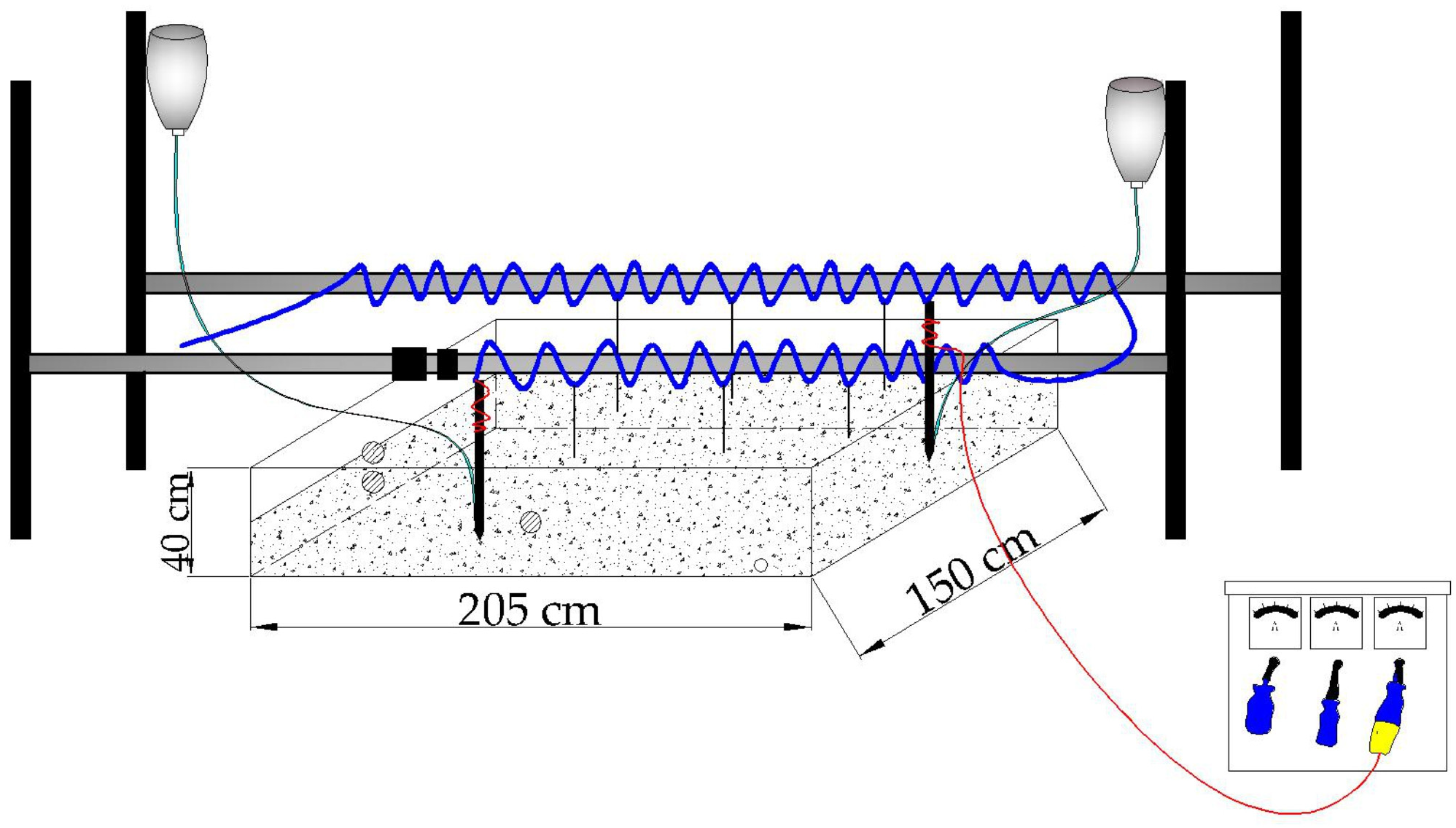
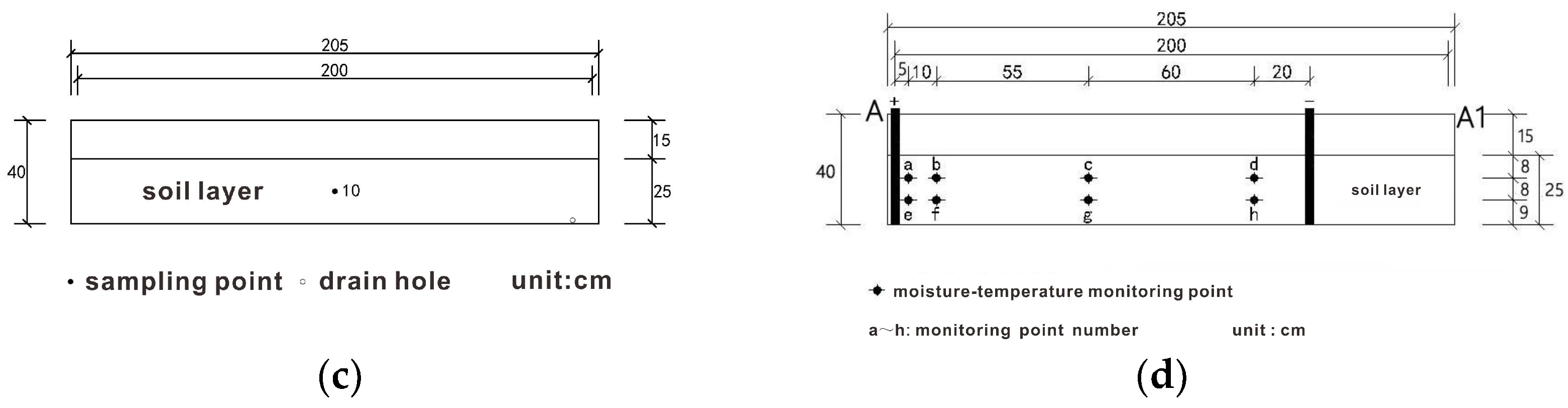
2.3. Experimental Setup and Procedure

The electric restoration experimental device consisted of five parts: power supply system, soil box solute transport system, conductive liquid spraying system, titration system and monitoring system. The power supply system consisted of a step-down transformer (with 5 A size ammeter) and two graphite electrodes. During the experiment, the wires representing the positive and negative electrodes were connected to the two graphite electrodes, and finally the two graphite electrodes were inserted into the soil vertically and slowly. The soil box solute transport system consisted of a Plexiglas box with dimensions of 205 cm × 150 cm × 40 cm (Length × Width × Height). The top of the soil box was not closed, and there was a drainage hole at the lower left corner of the front side, with several sampling holes punched on the front and left side according to the experimental needs for digging and taking soil samples. The conductive liquid spraying system consisted of a spraying head, a hose, a micro pump (flow rate 3.5 L/min), a reservoir and a timer. The spraying device was used to continuously spray 4 g/L NaCl solution into the soil; the spraying time interval was set to 1 h, and the duration of each spraying was 30 s, so that the soil was always kept wet during the experiment to improve the electrical conductivity of the soil. The titration system consisted of an infusion tube and an infusion bottle, one of which was filled with 0.1 mol/L NaOH solution as the alkaline titrant and the other with 0.1 mol/L citric acid solution as the acidic titrant. The titration rate of both the acidic and alkaline titrants was kept at about 4 drops/min during the experiment, which was a step taken to ensure the acid-base balance in the soil. The monitoring system was composed of a laptop computer and a high-precision multifunctional environmental sensor (which can monitor both temperature and moisture). The experimental setup is shown in Figure 1.

In this experiment, a total of 10 sampling points (Figure 2a–c) were set up from No. 1 to No. 10 to observe the changes in the content and migration of chromium heavy metal (hexavalent chromium) in the soil during the electric remediation process; a total of 8 moisture-temperature monitoring points (a~h) were set up at the central axis position (Section A-A1) to monitor the soil moisture content and soil temperature during the electric remediation process, with the aim of clarifying the changes in soil moisture content and soil temperature over time (Figure 2d). The step-down transformer has two outputs of 90 V and 110 V. Therefore, two sets of experiments were set up. Experiment 1: The voltage was 90 V, the electrode distance was 1.5 m, the soil height was 25 cm, and the experiment lasted for 7 days. The power was turned on at 10:30 a.m. on the first day and the first sample was taken before the power was turned on, after which the sample was taken once a day at 10:30 a.m. The data recording time interval of the monitoring system was 5 min. Experiment 2 set the voltage to 110 V and other parameters were the same.

2.4. Determination of Cr(VI) in Soil

In this experiment, the determination of Cr(VI) content in soil was carried out by diphenylcarbonyldihydrazide spectrophotometric method using UV-visible spectrophotometer. In the experiment, 0.2 g of diphenylcarbonyldihydrazide solid powder was weighed and dissolved in 50 mL of acetone, and subsequently diluted to 100 mL with water, shaken well and stored in a brown bottle under low temperature and light-proof conditions [30]. By weighing 0.2829 ± 0.0001 g of K₂Cr₂O₇ solid in water using an analytical balance, the solution was fixed in a 1000 mL volumetric flask and then diluted to 100 mL by taking 1 mL from the volumetric flask with water [31]. Subsequently, 1.00 mL, 2.00 mL, 4.00 mL, 8.00 mL, 10.00 mL, 15.00 mL, 20.00 mL and 25.00 mL were separated from the 100 mL of solution into eight 50 mL cuvette tubes by adding water slowly to the mark. After adding 50% sulfuric acid 0.5 mL, 50% phosphoric acid 0.5 mL and color developer 2.0 mL to each colorimetric tube, shaking well and leaving for 10 min, the solution was purplish red after adding the color developer [32]. The liquid was aspirated from each of the eight cuvettes into a 10 mm light range glass cuvette with the liquid height at approximately 2/3 of the height of the glass cuvette, after which the cuvette was placed in a UV-Vis spectrophotometer and the wavelength was adjusted to 540 nm to determine the absorbance value of each sample and plot the standard curve [33] (Figure 3).

After weighing 20.0 ± 0.05 g NaOH solid and 30.0 ± 0.05 g Na₂CO₃ solid with an analytical balance, they were dissolved in 500 mL deionized water and finally fixed in a 1000 mL volumetric flask and set aside [34]. After weighing 87.09 g K₂HPO₄ solid and 68.04 g KH₂PO₄ solid using an analytical balance, they were dissolved in 700 mL of deionized water and finally fixed in a 1000 mL volumetric flask and set aside [35].

The next step for the digestion was undertaken by weighing 2.5 ± 0.10 g of soil sample into a 250 mL conical flask using an analytical balance, followed by the addition of 50 mL of digestion solution, 0.4 g of MgCl₂ solid and 0.5 mL of phosphate buffer solution, shaking well for use [36]. The conical flask was placed in an oil-water bath for water bath heating, the temperature was adjusted to 93 °C and stirring was continued for 60 min during heating [37]. After heating and cooling to room temperature, it was placed in a syringe consisting of a 50 mL syringe connected to a 0.45 μm fibrous microporous membrane in a syringe-type filter with a replaceable membrane. The mixed liquid cooled to room temperature was filtered through the above filter into a 500 mL beaker and the pH was adjusted to between 7.0 and 8.0 by slowly adding 5.0 mol/L nitric acid with a rubber-tipped burette, a process controlled by a pH meter with an accuracy of 0.1 [38]. If a flocculent precipitate was produced, it was filtered again. Afterwards, the stirrer was removed and washed with deionized water, and the cleaned washing solution was transferred into the 500 mL beaker mentioned above. Finally, all the liquid in the beaker was transferred to a 250 mL volumetric flask and fixed with deionized water, shaking well for use [39].

In order to be measured after digestion, 50 mL of liquid was removed from the 250 mL volumetric flask in a 50 mL stoppered cuvette. After the addition of 50% sulfuric acid 0.5 mL, 50% phosphoric acid 0.5 mL and color developer 2.0 mL, the cuvette was shaken well and left for 10 min [40]. The liquid was aspirated from the cuvette into a glass cuvette of 10 mm optical range with a rubber-tipped dropper, and the height of the liquid was about 2/3 of the height of the glass cuvette, which was placed in a UV-Vis spectrophotometer and the wavelength was adjusted to 540 nm to determine the adsorbance value of each sample.

According to the standard curve, the concentration of Cr(VI) (µg/mL) was obtained and further conversion was carried out, as in Equation (1):

$$C=\frac{C_1\times V}{m}$$

(1)

In the equation, C is the concentration of Cr(VI) adsorbed in the soil (mg/kg); C₁ is the concentration of Cr(VI) obtained according to the standard curve (µg/mL); V is the volume of the volumetric flask when the volume is fixed after the soil digestion is completed, and it is 250 mL in this experiment; m is the mass of the soil sample used for digestion, which is 2.5 g in this experiment.

In order to quantitatively evaluate the effect of electrodynamic remediation of the polluted soil, it is necessary to calculate the removal rate of Cr(VI) at each observation point, as shown in Formula (2):

$$\rho =\frac{{\sigma }_1-{\sigma }_2}{{\sigma }_1-{\sigma }_0}\times 100\%$$

(2)

In the formula: ρ is the removal rate of hexavalent chromium of soil pollutants; σ₁ is the content of Cr(VI) before electrification; σ₂ is the content of Cr(VI) at the end of the test; σ₀ is the risk control value of hexavalent chromium of soil pollutants, taking the value of 5.7 μg/g.

2.5. Electric Repair Model

In this study, the multiphysics coupling finite element simulation software COMSOL MultiPhysics was used to solve the problem through the coupling of three physical fields, including “current”, “Richards equation” and “transfer of dilute substances in porous media” built in the software. The percentage content of sand, silt and clay, and soil physical properties such as soil bulk density were obtained through particle fractionation experiments and soil bulk density experiments. The data were input into RETC software, and the van Genuchten model was used for fitting. After running, the soil moisture characteristics were obtained. Some parameters related to pollutant transport were difficult to obtain through these experiments. This study referred to other literatures and empirical values for determination.

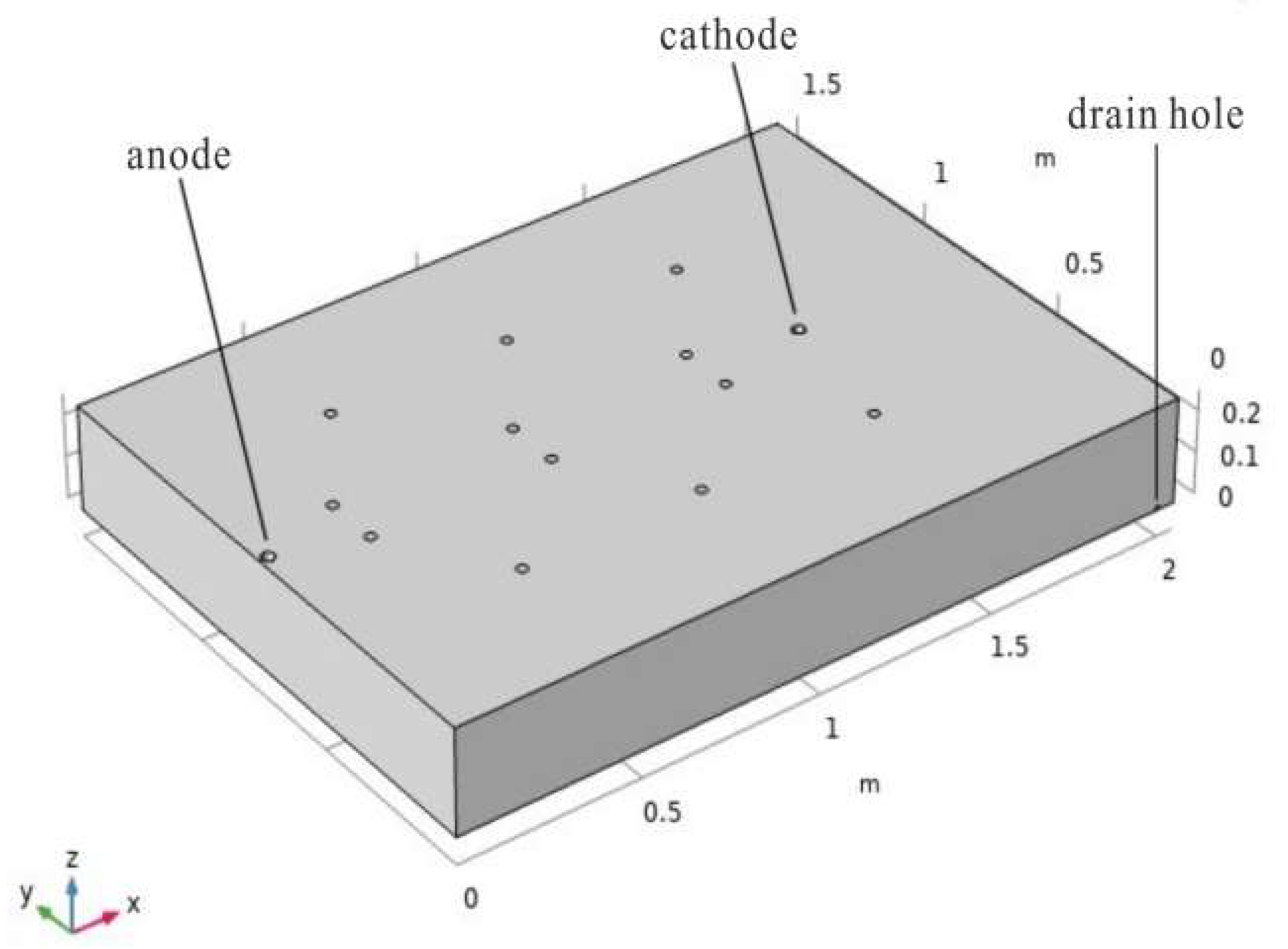
2.5.1. Model Establishment

According to the experimental process of electrokinetic remediation of unsaturated chromium-contaminated soil, a 1:1 3D model with the experimental device was established in COMSOL MultiPhysics (Figure 4). The soil size is 2.05 m × 1.5 m × 0.25 m. The location coordinates of the anode are (0.025, 0.75, 0), the radius is 0.0175 m, and it runs through the entire soil layer. The location coordinates of the cathode are (1.525, 0.75, 0), the radius is 0.0175 m, and it runs through the entire soil layer. There are 12 irrigation ports on the upper surface of the soil to simulate the water replenishment of the soil under the spray state. The coordinates of the water inlets are (0.45, 0.375, 0.25), (0.25, 0.675, 0.25), (0.95, 0.375, 0.25), (0.75, 0.675, 0.25), (1.45, 0.375, 0.25), (1.25, 0.675, 0.25), (0.45, 1.125, 0.25), (0.25, 0.825, 0.25), (0.95, 1.125, 0.25), (0.75, 0.825, 0.25), (1.45, 1.125, 0.25), (1.25, 0.825, 0.25), and the radius of the irrigation outlet is 0.005 m. The soil layer has a drainage outlet near the bottom surface. The coordinates of the drainage outlet are (2.00, 0, 0.01) and the radius is 0.005 m.

2.5.2. Setting Observation Points and Time Steps

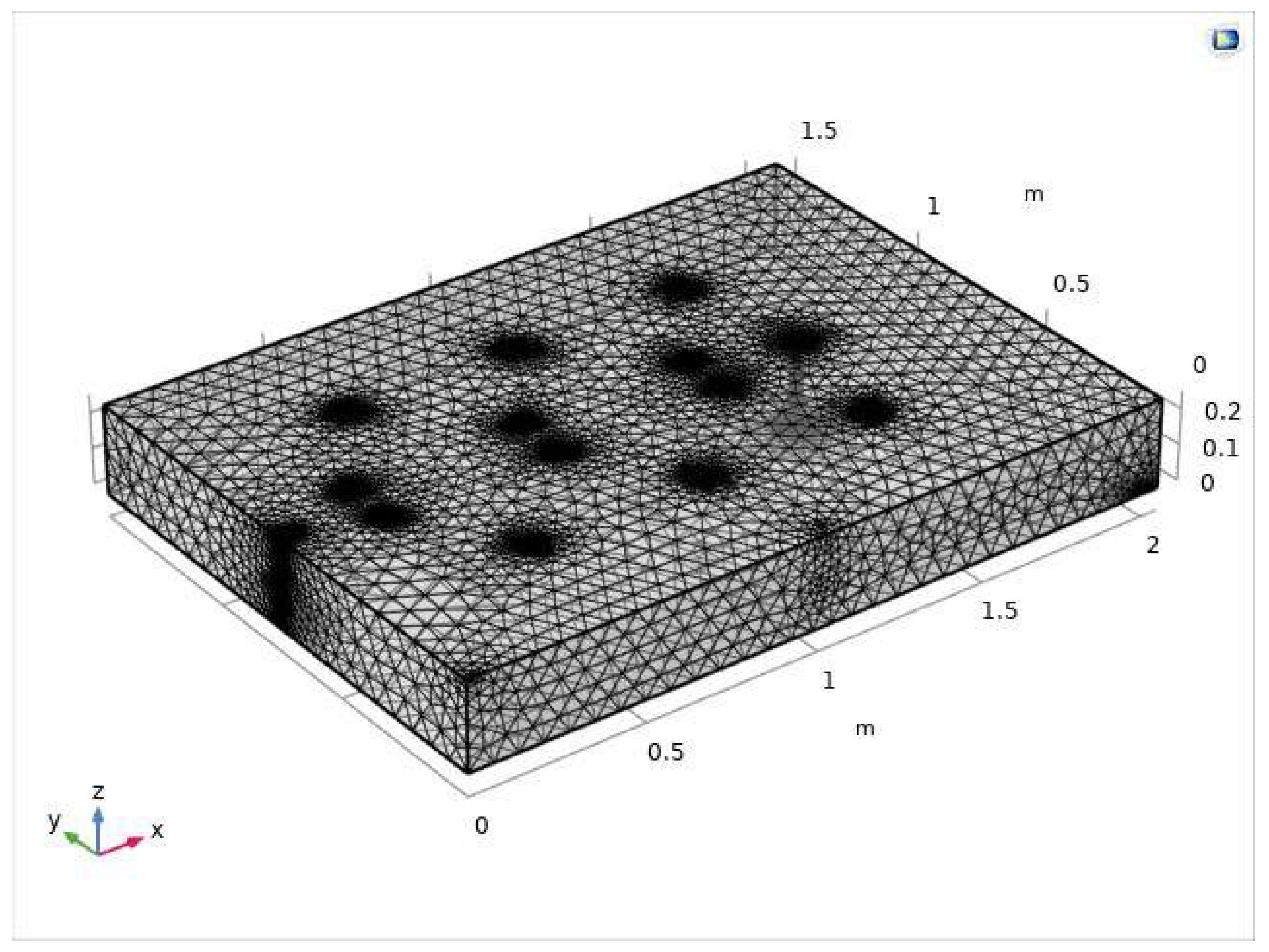
The number of observation points is consistent with the laboratory test (Figure 5). The position coordinates of the moisture monitoring points a~h are a (0.075, 0.75, 0.17), b (0.175, 0.75, 0.17), c (0.725, 0.75, 0.17), d (1.325, 0.75, 0.17), e (0.075, 0.75, 0.09), f (0.175, 0.75, 0.09), g (0.725, 0.75, 0.09), h (1.325, 0.75, 0.09). The position coordinates of sampling points 1, 2, 3, 6, and 7 are 1 (0.075, 0.7, 0.25), 2 (0.125, 0.7, 0.25), 3 (0.175, 0.7, 0.25), 6 (0.725, 0.7, 0.25), 7 (1.325, 0.7, 0.25). The simulation period is 168 h (7 days), the initial time is 0 h, the simulation end time is 168 h, and the time step is 1 h.

2.5.3. Meshing

Using the physical field control mesh, the finite element mesh is dissected by selecting the hyperfine cell size for the soil body, and the complete dissected mesh contains 163,626 domain cells, 17,454 boundary elements and 1031 edge cells (Figure 6).

2.5.4. Model Boundary Conditions

In order to simulate the infiltration of sodium chloride solution and the transport of contaminants during the experiment, the irrigation port of the model was set as the constant head boundary, and the sodium chloride solution was injected every 1 h with a duration of 30 s for each injection by customizing the pulse curve. The drainage port of the model is defined as the free outflow boundary. The other boundaries of the model are defined as no-flow boundaries.

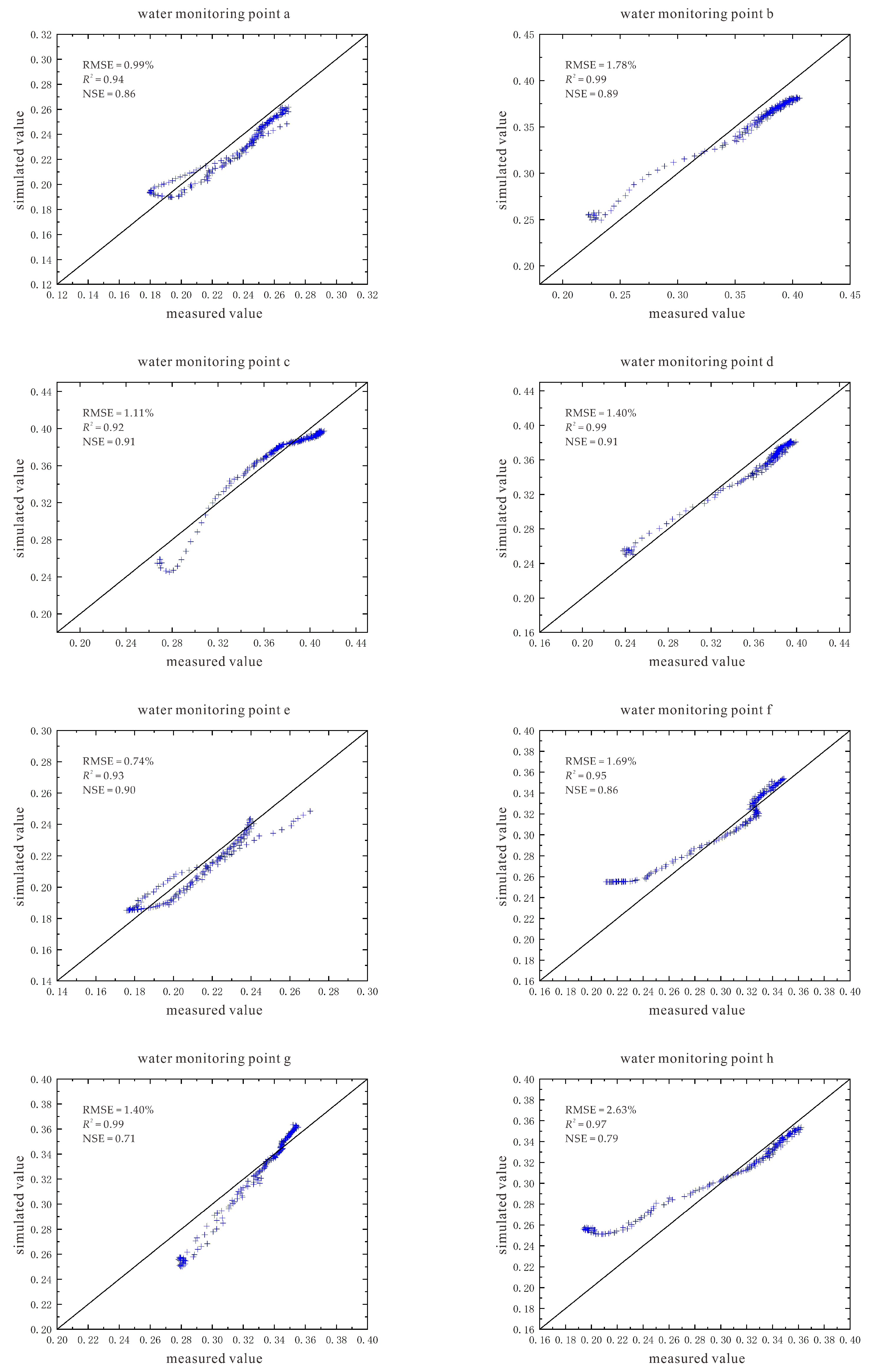
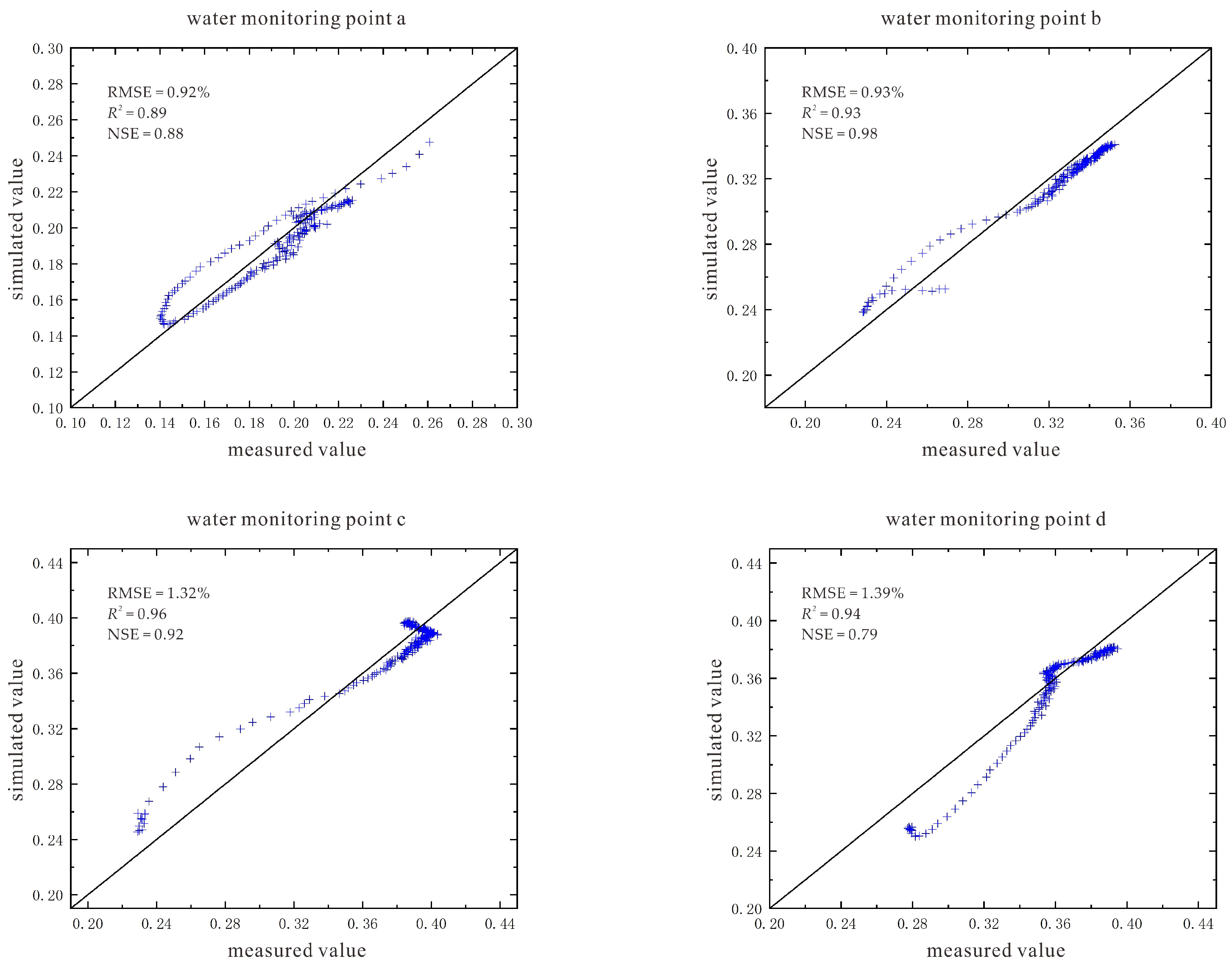
2.5.5. Model Evaluation Indicators

In order to evaluate the reliability of the model, this study uses RMSE (root mean square error), R² (determination coefficient of correlation between data) and NSE (Nash efficiency coefficient) to evaluate the model.

The RMSE formula is as follows. The closer the RMSE value is to 0, the better the fit between the measured value and the simulated value, and the higher the reliability of the model.

$$\mathrm{RMSE}=\sqrt{\frac{1}{n}{\displaystyle \sum }_{i=1}^n{\left(S_i-O_i\right)}^2}$$

(3)

The R² formula is as follows. The closer the value of R² is to 1, the greater the correlation between the measured value and the simulated value, and the higher the fitting degree. In this study, if R² > 0.9, the model is considered to be well fitted.

$$R^2=\frac{{\left[{\displaystyle {\displaystyle \sum }_{i=1}^n}\left(S_i-\overline{S}\right)\left(O_i-\overline{O}\right)\right]}^2}{{\displaystyle {\displaystyle \sum }_{i=1}^n}{\left(S_i-\overline{S}\right)}^2{\displaystyle {\displaystyle \sum }_{i=1}^n}{\left(O_i-\overline{O}\right)}^2}$$

(4)

The NSE formula is as follows. The closer the NSE value is to 1, the smaller the error between the measured value and the simulated value. In general, if NSE > 0.5, the model is considered to meet the requirements.

$$\mathrm{NSE}=1-\frac{{\displaystyle {\displaystyle \sum }_{i=1}^n}{\left(S_i-O_i\right)}^2}{{\displaystyle {\displaystyle \sum }_{i=1}^n}{\left(O_i-\overline{O}\right)}^2}$$

(5)

In the formula, n represents the number of data; $S_i$ represents the ith simulated value; $O_i$ represents the ith measured value; $\overline{S}$ represents the average value of the simulated value; $\overline{O}$ represents the average value of the measured value.

3. Results and Discussion

3.1. Experimental Analysis

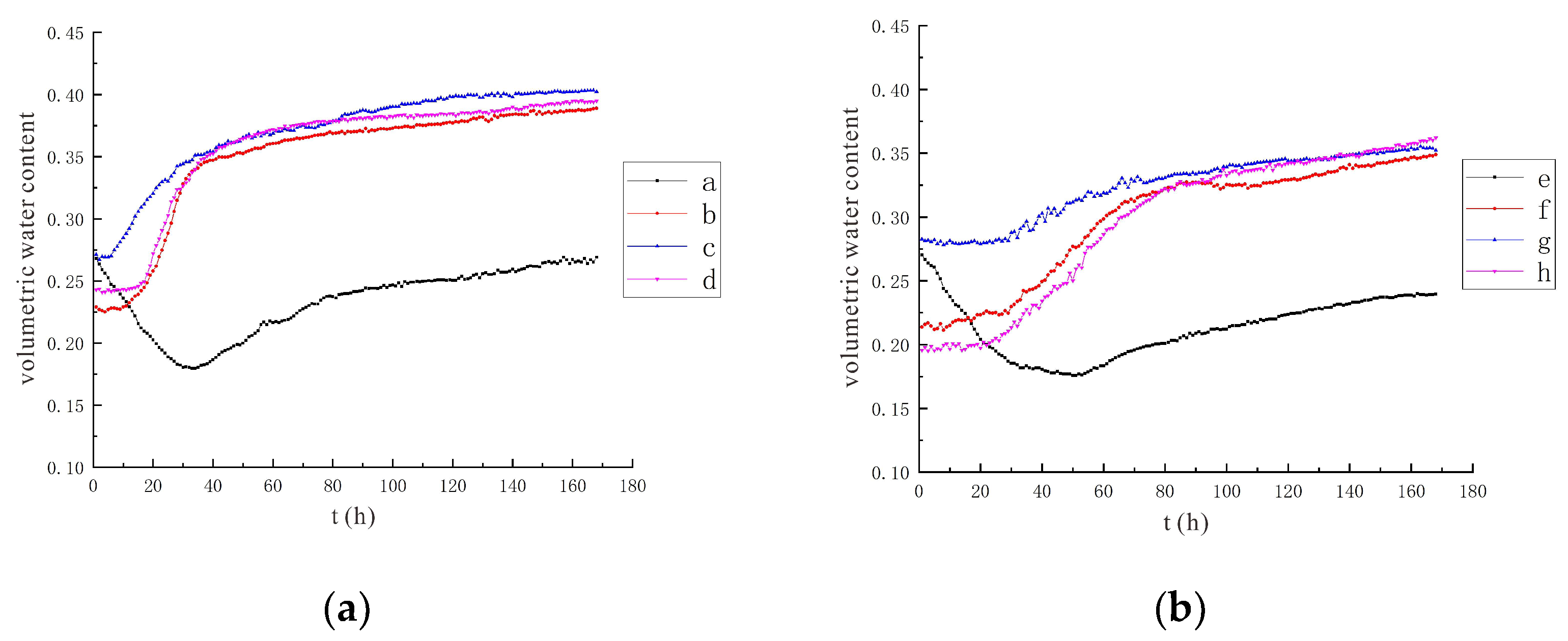
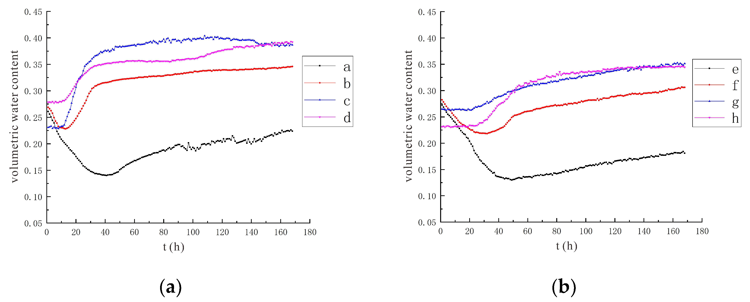
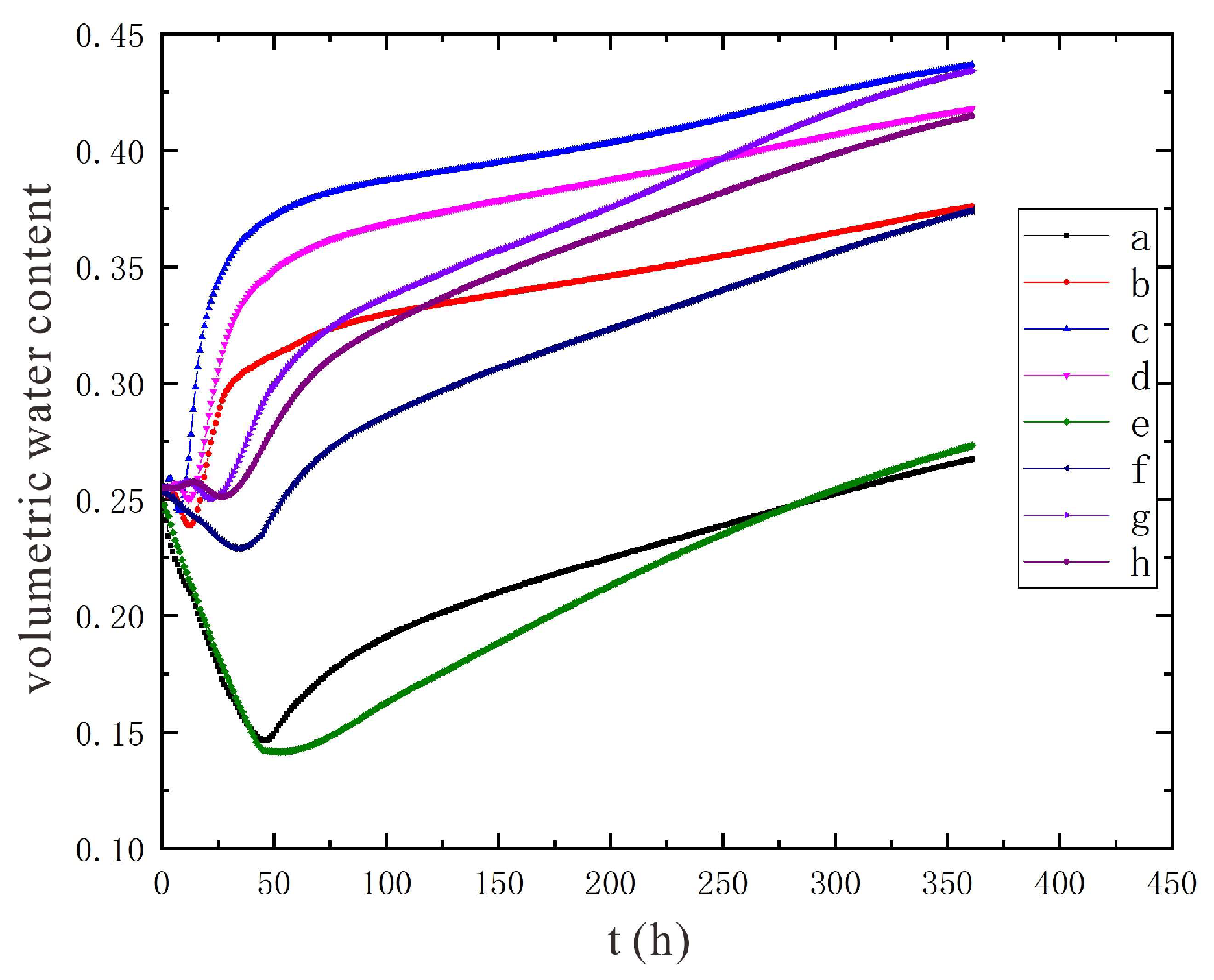
3.1.1. Characteristics of Soil Moisture Distribution

It can be concluded from the data (Figure 7 and Figure 8) that under the condition of a voltage of 90 V, the influence range of the electrolysis reaction is limited, and the water monitoring points b and f are less affected, mainly by the diffusion of the injected solution at the irrigation port. The area of influence expands, causing the soil moisture at these two points to be electrolyzed and to reduce the soil volumetric moisture content. When the solution injected into the irrigation port diffuses here, the influence of the solution diffusion is greater than that of the electrolysis reaction, and the soil volumetric water content increases. For other monitoring points, the volumetric water content at point a decreased by 8.9% in the 90 V condition and by 12.0% in the 110 V condition. The volumetric water content at point e decreased by 9.4% in the 90 V condition and by 14.4% in the 110 V condition. It can be concluded that the greater the voltage, the greater the electric field strength, the higher the efficiency of water electrolysis, and the greater the reduction of soil volumetric water content.

It has been experimentally demonstrated that the high field strength soil environment enhanced the electrodialysis process and increased the ion migration rate in pore water, which indirectly facilitated the removal of heavy-metal-like contaminants [41]. This is similar to the monitoring of soil moisture changes in this study, which also provides support for this experiment, demonstrating that elevated voltage can indeed accelerate soil moisture transport, thus helping to improve the removal of heavy metal chromium.

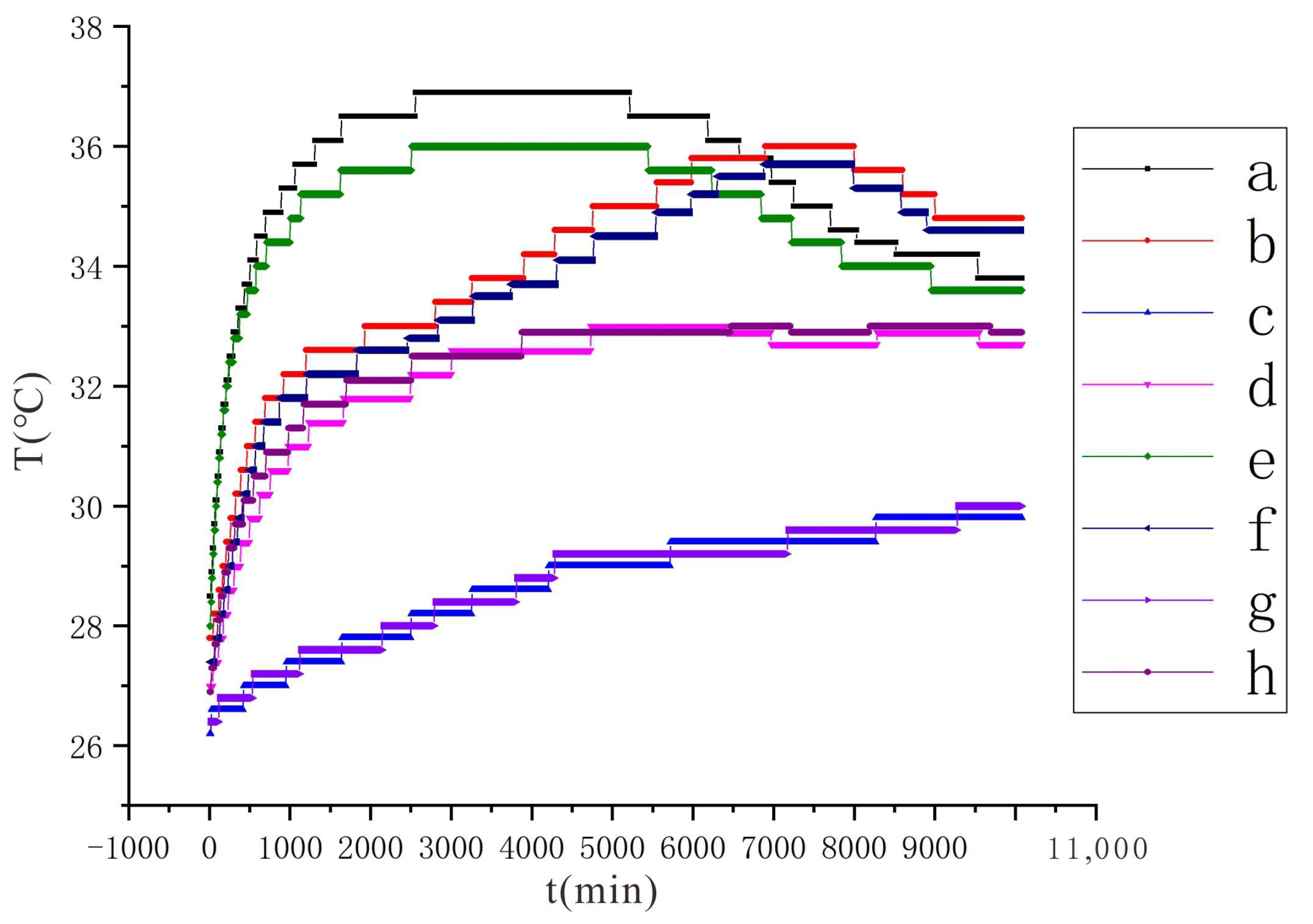
3.1.2. Characteristics of Soil Temperature Change

Comparing the experimental results under different voltage conditions (Figure 9 and Figure 10), in the initial temperature rise stage, the temperature rise rate and maximum value of the monitoring points at the same position under the condition of 110 V are larger than those under the condition of 90 V. Additionally, under the two conditions a (or e) reaches the maximum value and the trough minimum value earlier than b (or f). The reason for the analysis is that the amount of conductive liquid sprayed under the two conditions is the same, and the ability to electrolyze water is stronger under the condition of 110 V, so the moisture in the soil will drop faster. Once the water is insufficient, the electrolytic reaction will weaken and the soil temperature will also drop. After a period of time, the continuously sprayed conductive liquid is enriched in the soil to increase the water content, and the electrolysis reaction will increase again with the enhanced temperature.

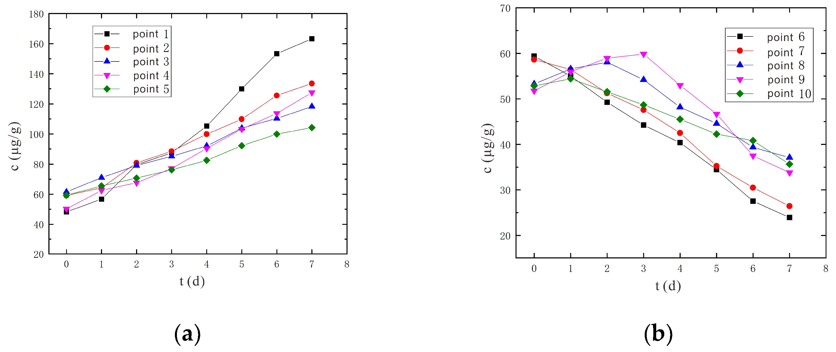
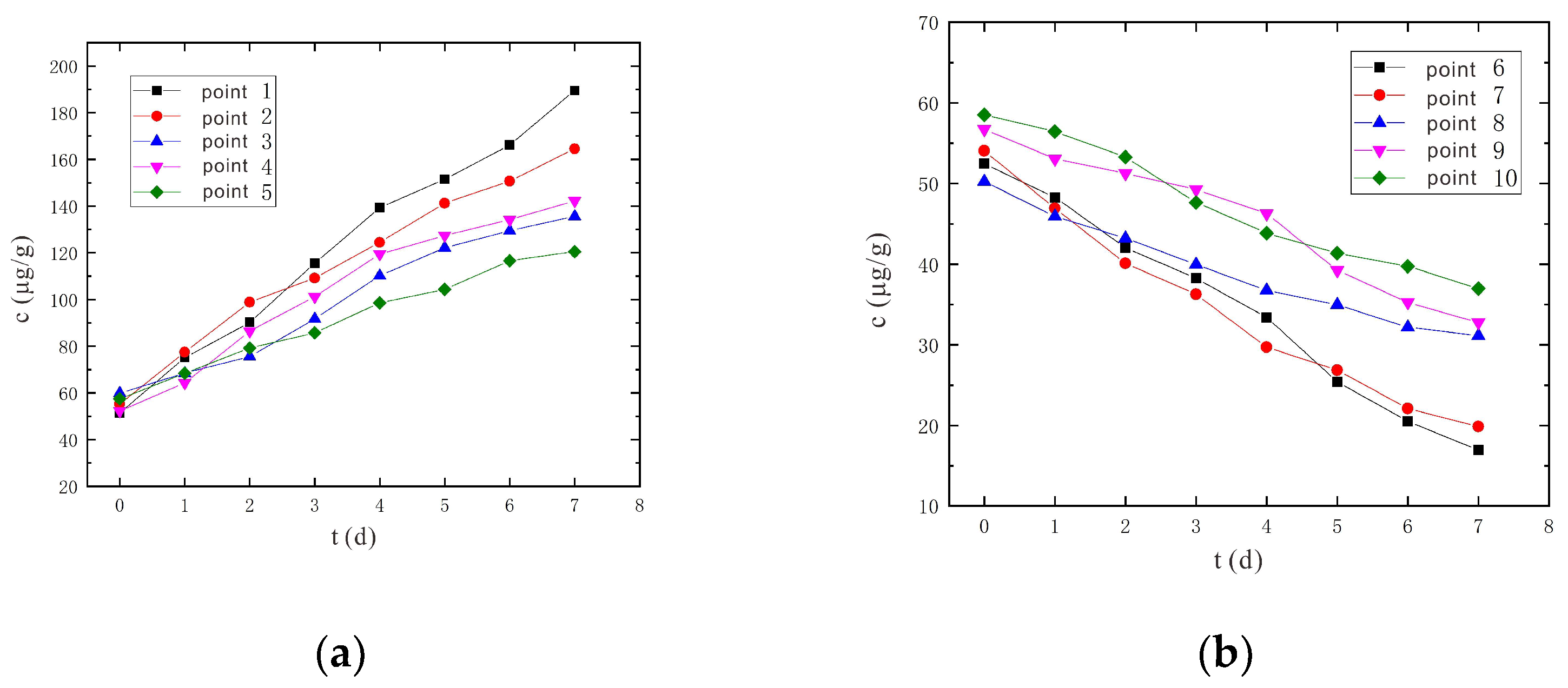
3.1.3. Variation Characteristics of Hexavalent Chromium Concentration

From Figure 11 and Figure 12, it can be found that the Cr(VI) concentrations at sampling points 6 and 7 both decreased continuously at a voltage of 90 V and an electrode distance of 1.5 m. However, there were peaks during the change of Cr(VI) concentrations at sampling points 8 to 10, and the peak times were also different. The earliest peak occurrence was at sampling point 10, followed by sampling point 8, and the latest peak occurrence was at sampling point 9. Nevertheless, under the conditions of a voltage of 110 V and an electrode distance of 1.5 m, the Cr(VI) concentration of No. 6~10 sampling points continued to decrease and no peak appeared. The reason for this phenomenon is analyzed as such: the Cr(VI) in any part of the soil leaves due to migration on the one hand, and at the same time accepts the nearby Cr(VI); the content of Cr(VI) is a dynamic change process. When the electric field strength and current density are small, the migrated Cr(VI) is less than the accepted Cr(VI), so the Cr(VI) content increases; when the electric field strength and current density are large, the amount of migrated Cr(VI) is larger than the incoming Cr(VI), so the Cr(VI) content tends to decrease. Under the conditions of a voltage of 90 V and an electrode distance of 1.5 m, because the voltage is relatively low, and the sampling points 8~10 are far away from the anode and cathode electrodes, the electric field strength and current density are relatively small. Thus, the amount of received Cr(VI) will be larger than in the case of migrating Cr(VI), and the concentration of Cr(VI) increases with a peak. Under the conditions of a voltage of 110 V and an electrode distance of 1.5 m, due to the relatively high voltage, the electric field strength and current density are also relatively large, and the levels of migrated Cr(VI) will be larger than the received Cr(VI), so Cr(VI) concentrations will continue to drop without peaks.

In the table: ρ is the removal rate of soil pollutant hexavalent chromium; σ₁ is the content of Cr(VI) before electrification; σ₂ is the content of Cr(VI) at the end of the test; σ₀ is the risk control value of soil pollutant hexavalent chromium and the value is 5.7 μg/g.

It can be found from

Table 1. Parameters related to the removal rate of Cr(VI) at sampling points 6–10 in the two groups of experiments.

Sampling Point Number	σ1 (μg/g)	σ2 (μg/g)	σ0 (μg/g)	ρ (%)
Sampling point 6 (90 V, 1.5 m)	59.38	23.94	5.7	66.03
Sampling point 7 (90 V, 1.5 m)	58.64	26.45	5.7	60.80
Sampling point 8 (90 V, 1.5 m)	53.28	37.10	5.7	34.01
Sampling point 9 (90 V, 1.5 m)	51.78	33.81	5.7	40.00
Sampling point 10 (90 V, 1.5 m)	52.86	35.67	5.7	36.44
Sampling point 6 (110 V, 1.5 m)	52.45	16.94	5.7	75.96
Sampling point 7 (110 V, 1.5 m)	54.08	19.86	5.7	70.74
Sampling point 8 (110 V, 1.5 m)	50.26	31.14	5.7	42.90
Sampling point 9 (110 V, 1.5 m)	56.72	32.78	5.7	46.93
Sampling point 10 (110 V, 1.5 m)	58.53	36.97	5.7	40.81

that for the sampling points 6 to 10, the removal rate of Cr(VI) at the corresponding sampling points at the same position under the two conditions is greater under the condition of 110 V than that under the condition of 90 V. Higher voltages can improve the removal of hexavalent chromium, which is consistent with the findings of previous articles [21]. This demonstrates the feasibility of increasing the voltage to enhance the electroremediation efficiency.

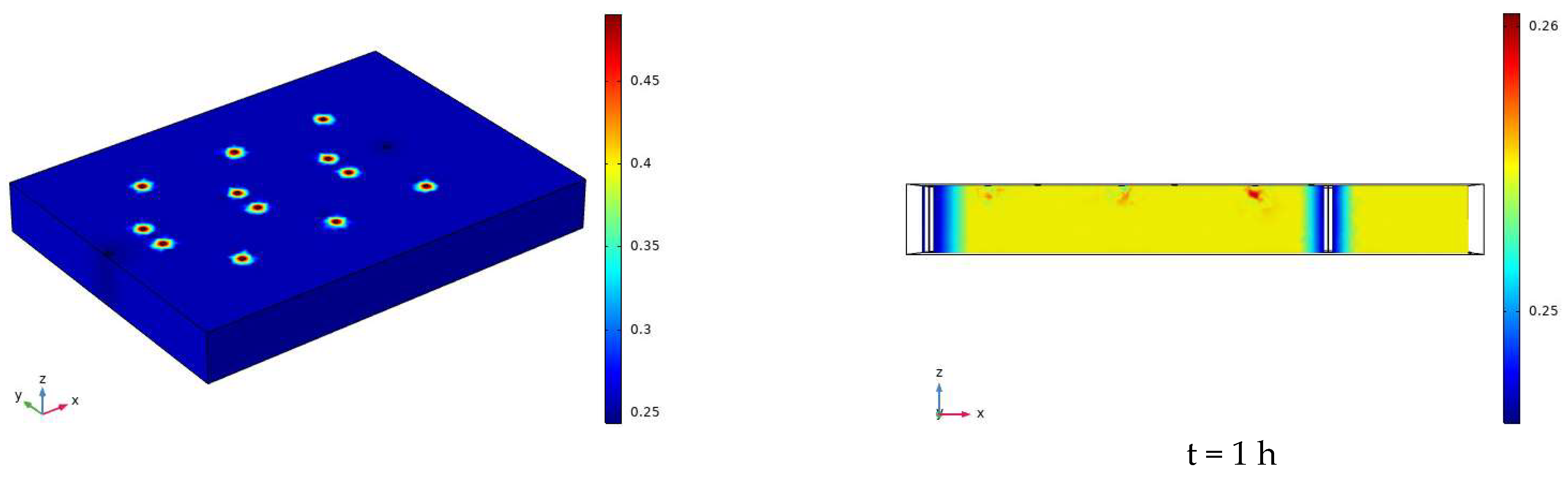
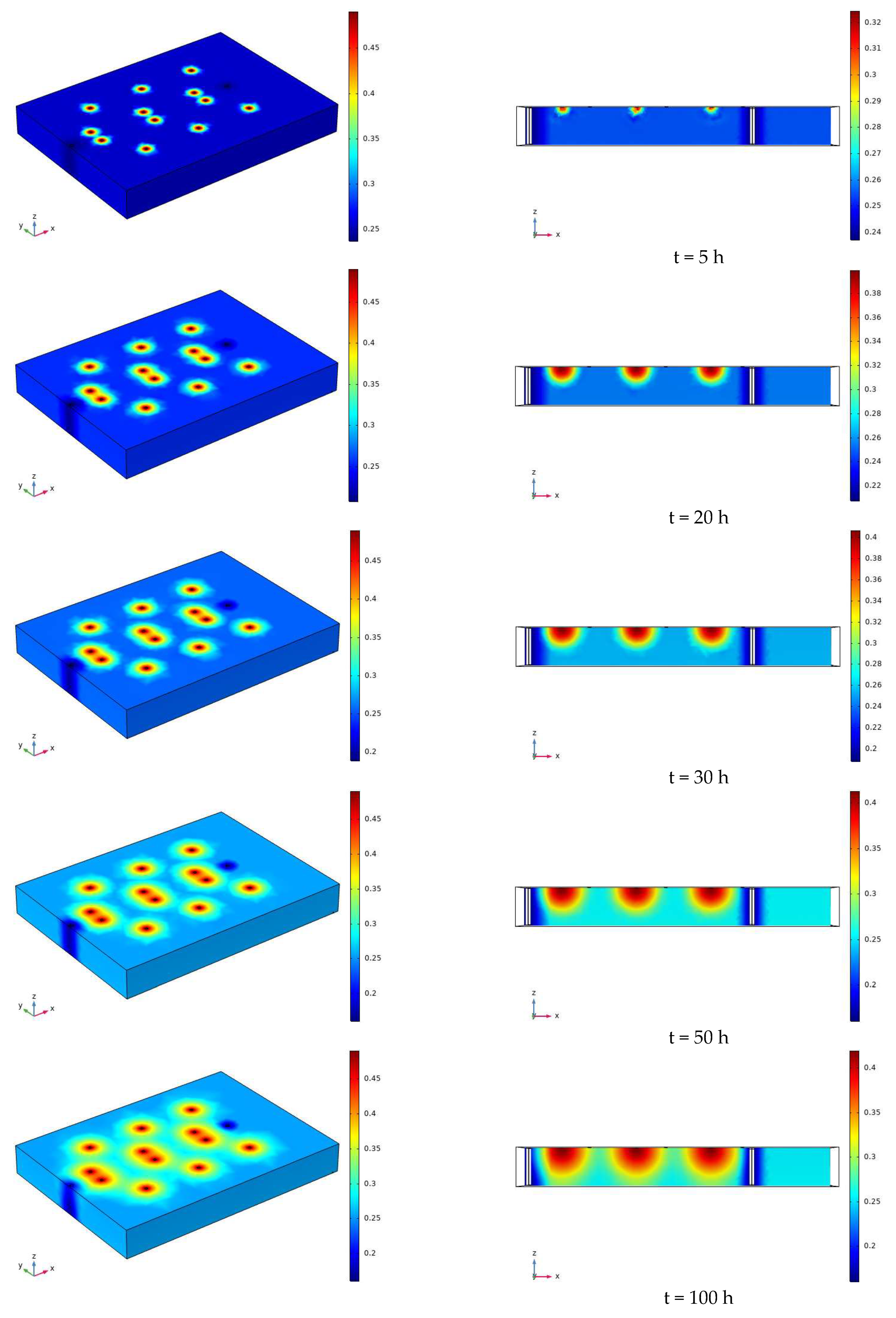
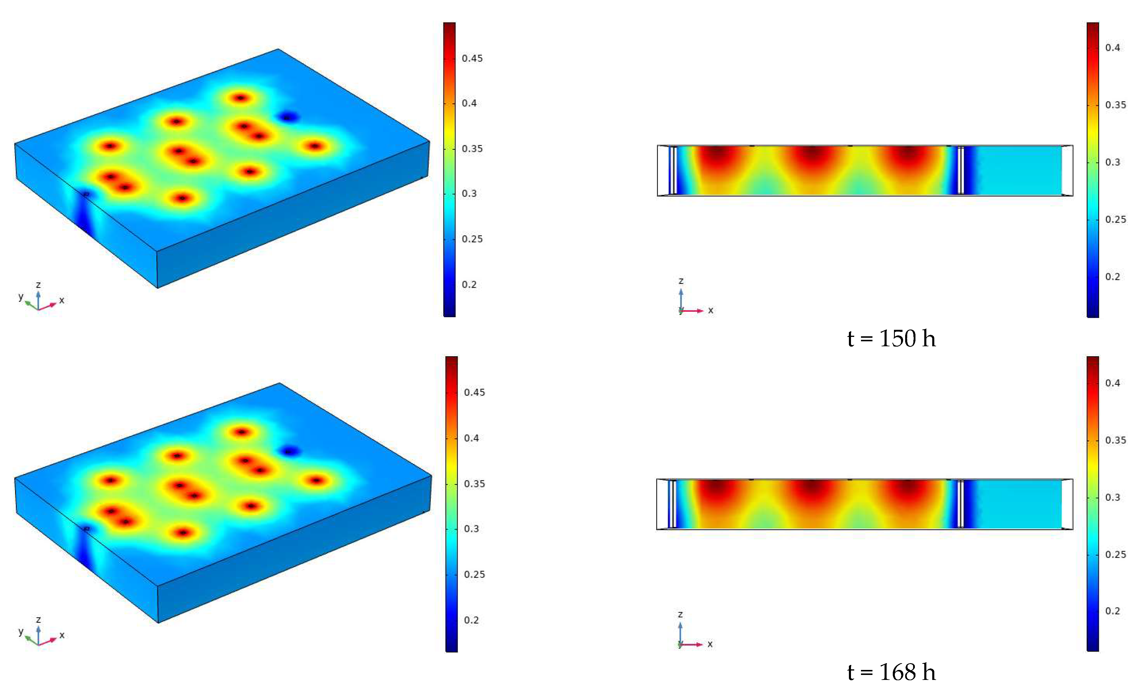
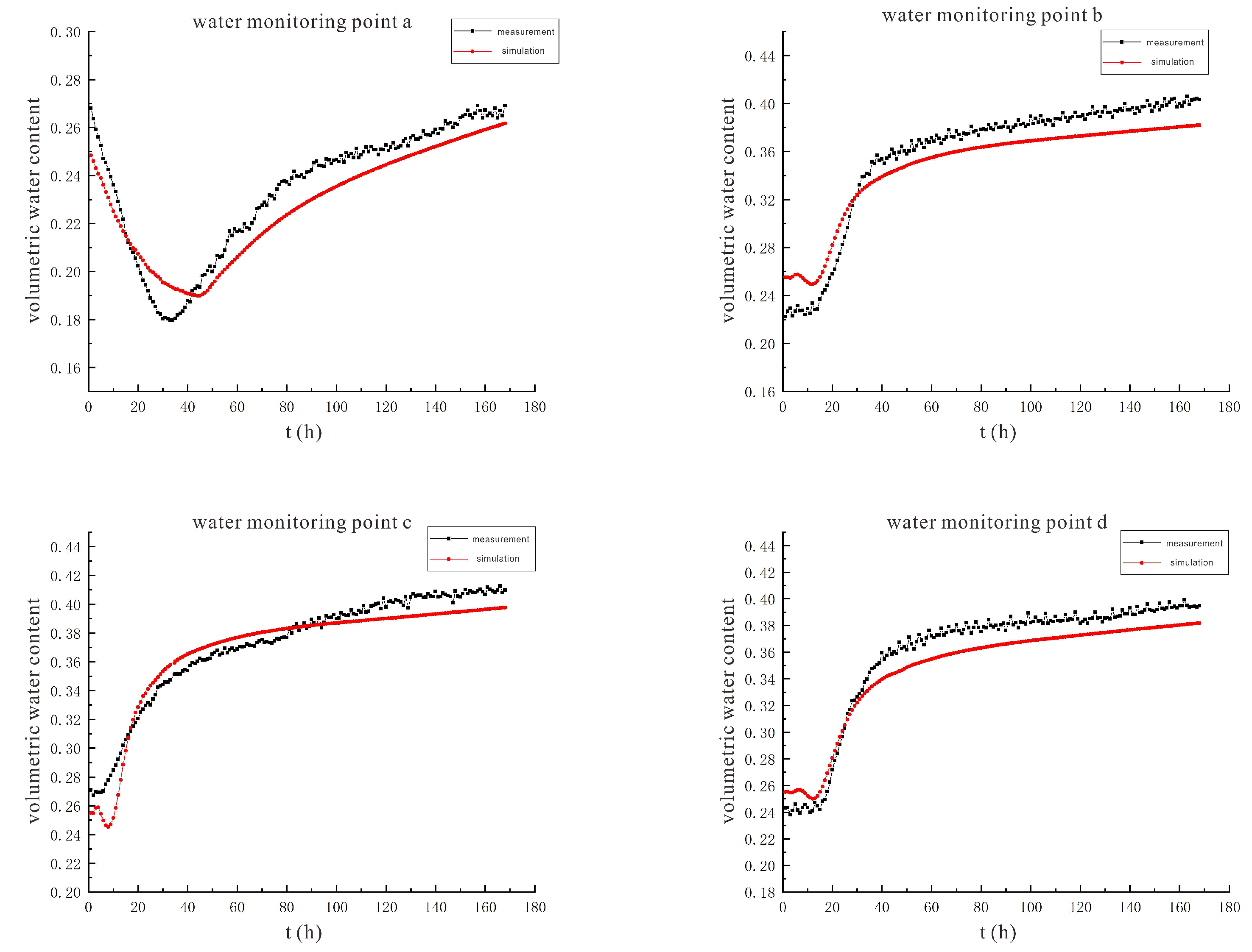
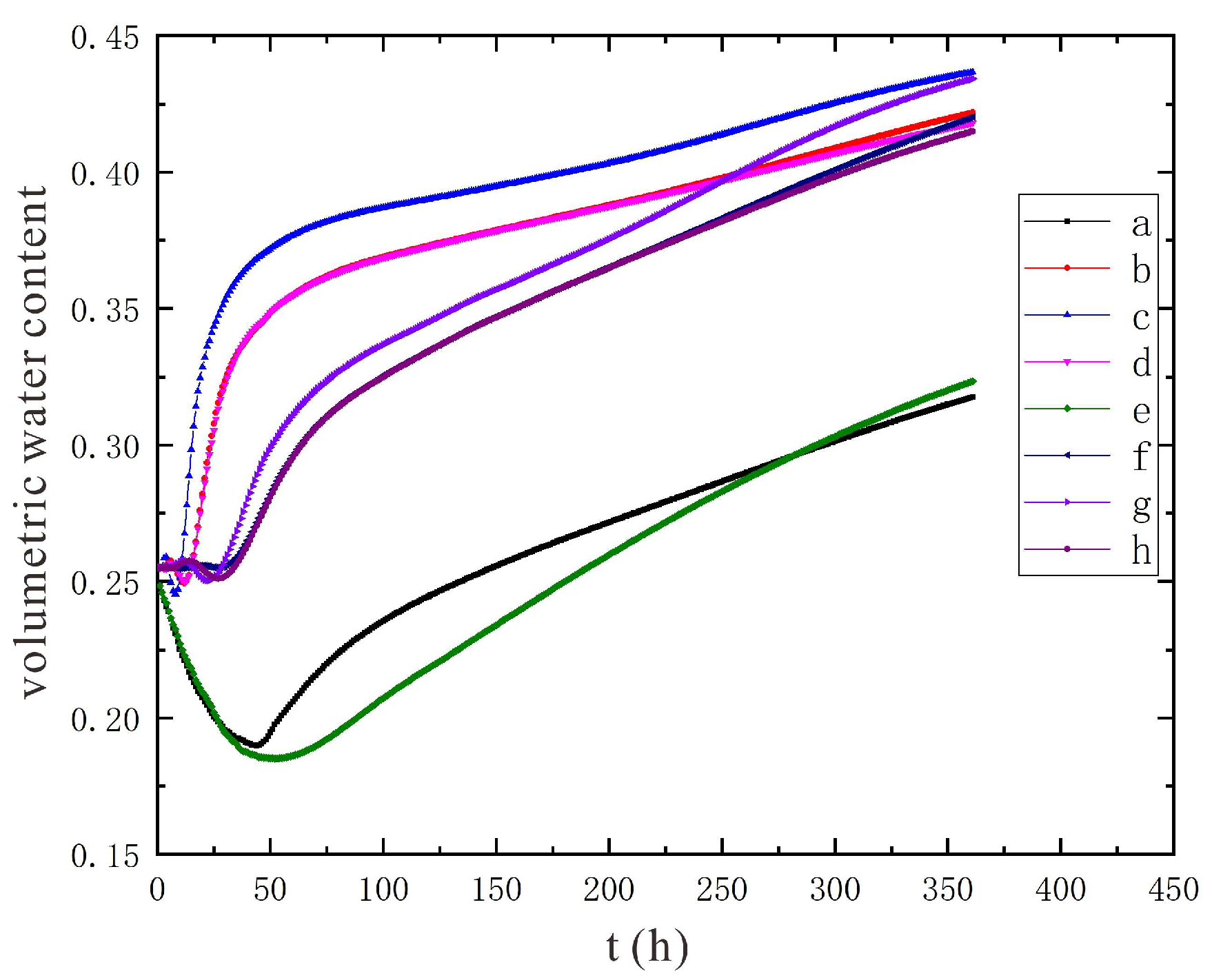
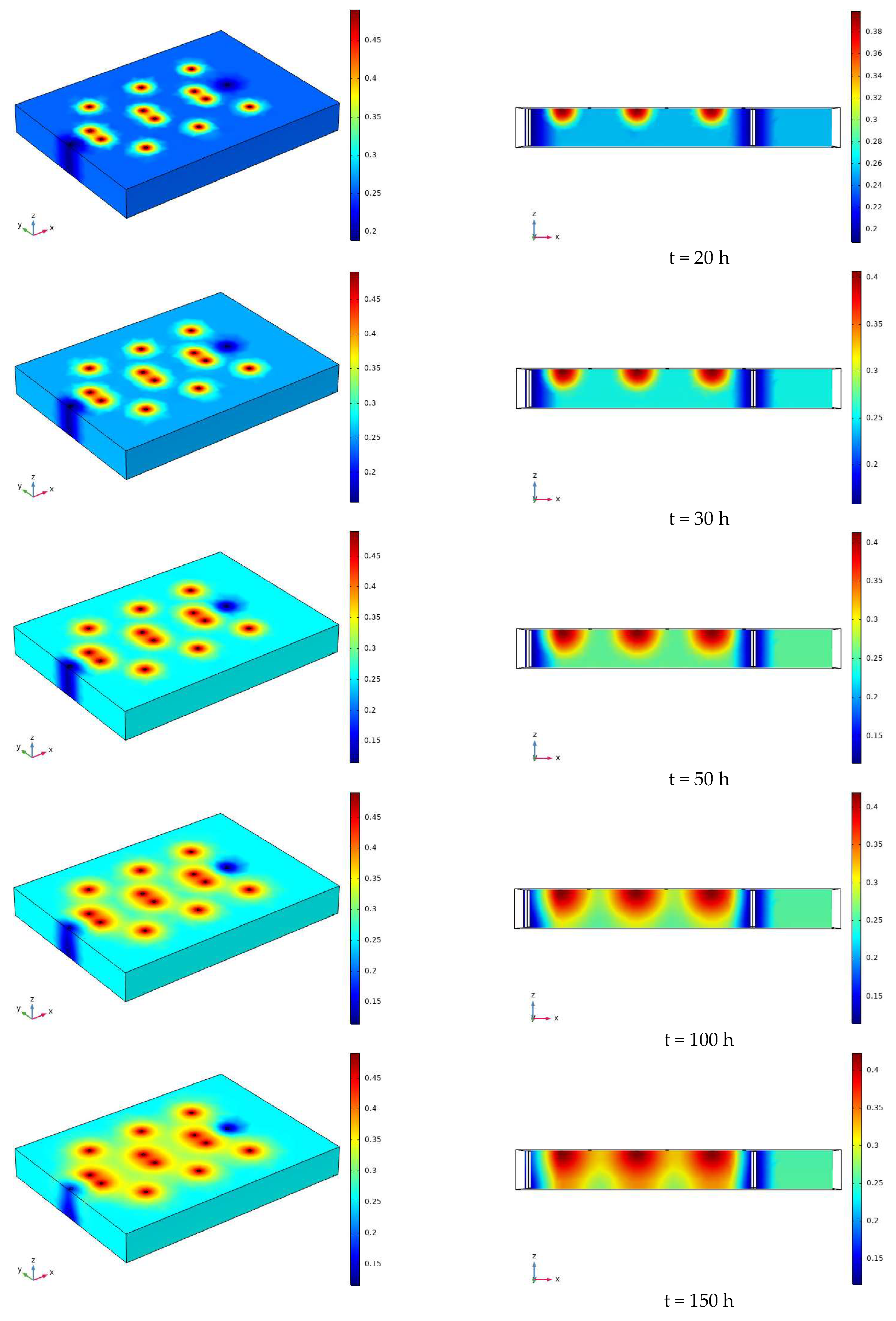
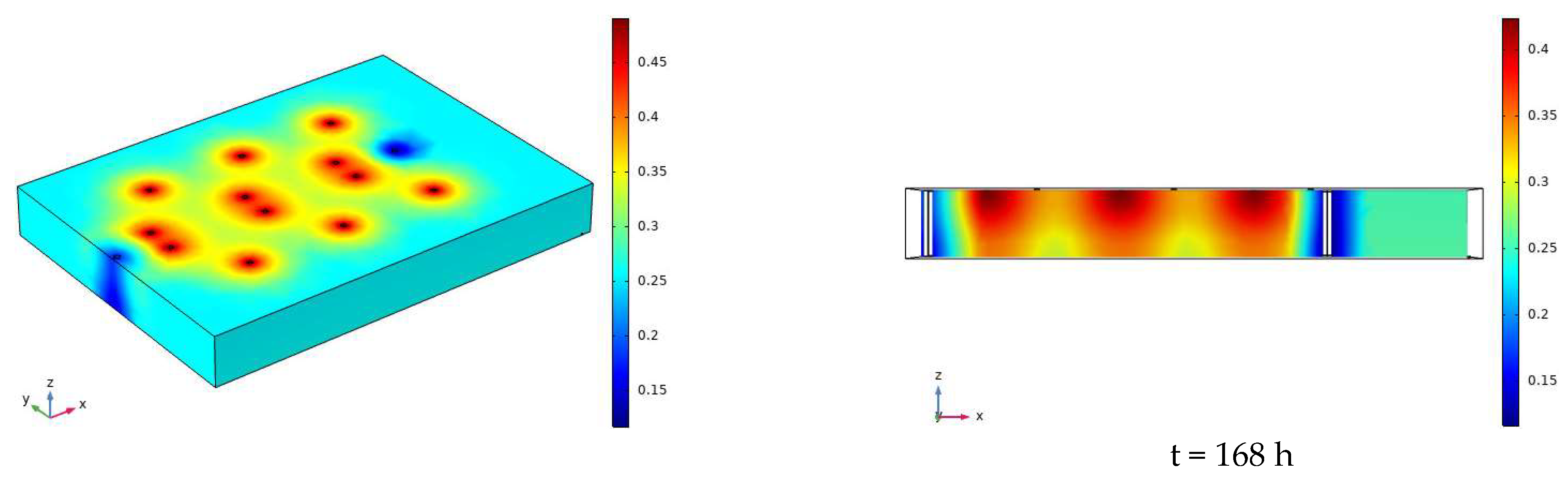
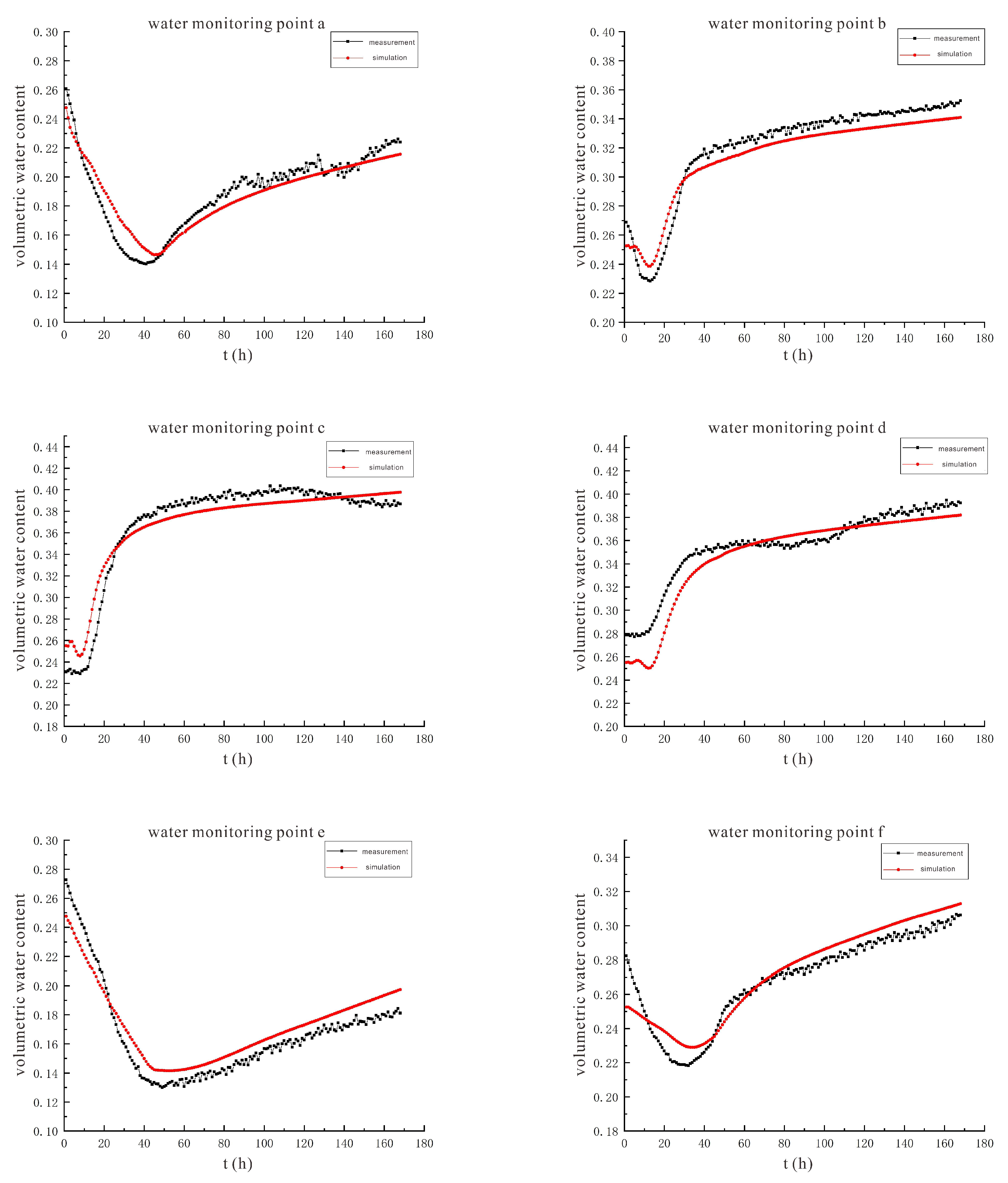
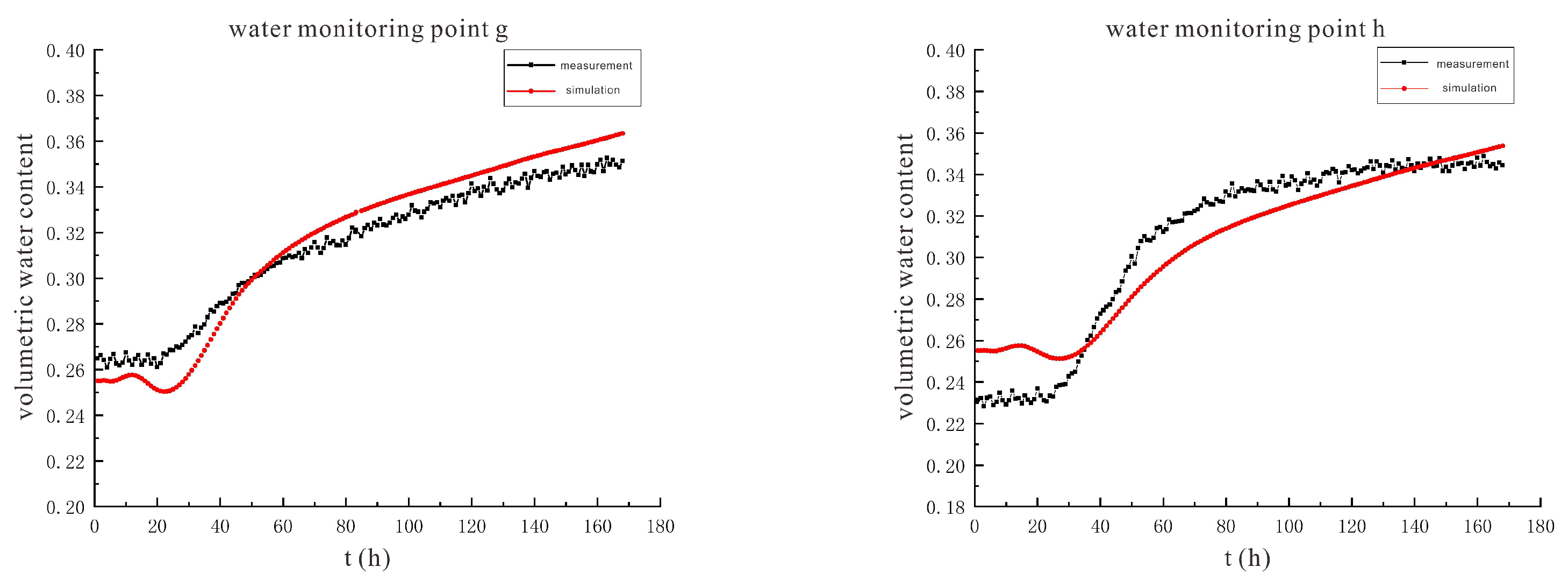
3.2. Characteristics of Model Soil Moisture Distribution

3.2.1. Voltage 90 V, Electrode Distance 1.5 m

The water distribution cloud map of the infiltration of sodium chloride solution under the conditions of 90 V and 1.5 m for 7 days (168 h) is shown in Figure 13. As time goes on, water begins to diffuse from each irrigation outlet to the surrounding concentric circles. During the diffusion process, the soil volumetric water content near the center point is the highest, which is close to the saturated water content of 48%. The closer to the outer layer, the lower the soil volumetric water content. Each water filling port is at a certain distance from the electrode. At 168 h, the water basically diffuses to the position of the electrode. The electrolysis reaction near the electrode has a certain range. When the water diffuses to the vicinity of the electrode, the transport and removal of water near the electrode is not affected by the electrolysis, and will also be affected by the water diffusion. Figure 13 only reflects the changes of moisture on the soil surface and profile, and cannot quantitatively study the soil volumetric moisture content for specific moisture monitoring points. Therefore, the data obtained from the simulation of each moisture monitoring point are derived from COMSOL, and then compared with the measured data. The comparison curve of the measured and simulated soil volume water content is shown in Figure 14.

Figure 14 shows that under the conditions of 90 V and 1.5 m, the measured and simulated values of soil volumetric water content at water monitoring points a~h have similar trends but there is a certain gap between them. The main reasons for the analysis are: I. The initial volumetric water content of the soil set by the simulation is the same in all positions of the soil, which is 25.5%. In the laboratory test, the initial soil volumetric water content was different in different positions of the soil. II. The simulation does not take into account the effect of evaporation of water from the soil. The indoor test was in summer, the temperature was high, and under the action of the electric field, the electrolysis reaction in the soil would release heat, which would increase the soil temperature, and the evaporation of water in the soil would also increase. III. During the soil filling process of the indoor test, there will be uneven filling, resulting in many cracks in the soil. Preferential flow occurs when the solution is injected, where rapid infiltration of the solution from large channels in the soil occurs.

Figure 15 shows the simulation results and evaluation indicators of soil volumetric water content under the conditions of 90 V and 1.5 m, which are used to quantitatively evaluate the reliability of the distribution of soil volumetric water content calculated by the model. The RMSE (root mean square error) values of the moisture monitoring points a~h are between 0.74% and 2.63%, the R² (determination coefficient of correlation between data) values are between 0.92 and 0.99, and the NSE (Nash efficiency coefficient) values are between 0.71 and 0.93. The three indicators all indicate that the simulation effect of each point is good, and the model has high reliability.

According to the established model, the change of the volumetric water content at points a~h under the conditions of 90 V and 1.5 m in 360 h (15 days) is predicted (Figure 16). Comparing the trend of water changes at each water monitoring point, it is found that the soil volumetric water content at the shallower depths is initially greater than that at the deeper depths. However, with the growth of time, the gap between the two will gradually narrow, and finally the volumetric water content of the soil at a deeper depth will be greater than that at a shallower depth.

3.2.2. Voltage 110 V, Electrode Distance 1.5 m

The water distribution clouds of NaCl solution infiltration at 110 V and 1.5 m for 7 days (168 h) are shown in Figure 17. Comparing Figure 17 with Figure 13, it can be found that the degree of water reduction near the cathode and anode electrodes is greater at 110 V than at 90 V, and the radius of the area of volume water content reduction near the electrodes is also greater than at 90 V.

Continuing the previous operation, the simulated data and the measured data are compared and analyzed to obtain the soil volumetric moisture content comparison curve in Figure 18.

The variation trends of the measured and simulated values of soil volumetric water content at each monitoring point under the condition of 110 V are similar to those under the condition of 90 V, and the reasons for the two are the same.

The simulation results and evaluation indicators of soil volumetric water content are also given (Figure 19). The RMSE (root mean square error) values of the water monitoring points a~h are between 0.84% and 1.39%, and the R² (determination coefficient of correlation between data) is between 0.89 and 0.99, and the NSE (Nash efficiency coefficient) value is between 0.79 and 0.98. These three indicators all indicate that the simulation effect of each point is good, and the model has high reliability.

The moisture prediction diagram under the conditions of 110 V and 1.5 m is shown in Figure 20. Comparing the trend of moisture change at each point, the same results can be obtained as under the conditions of 90 V and 1.5 m.

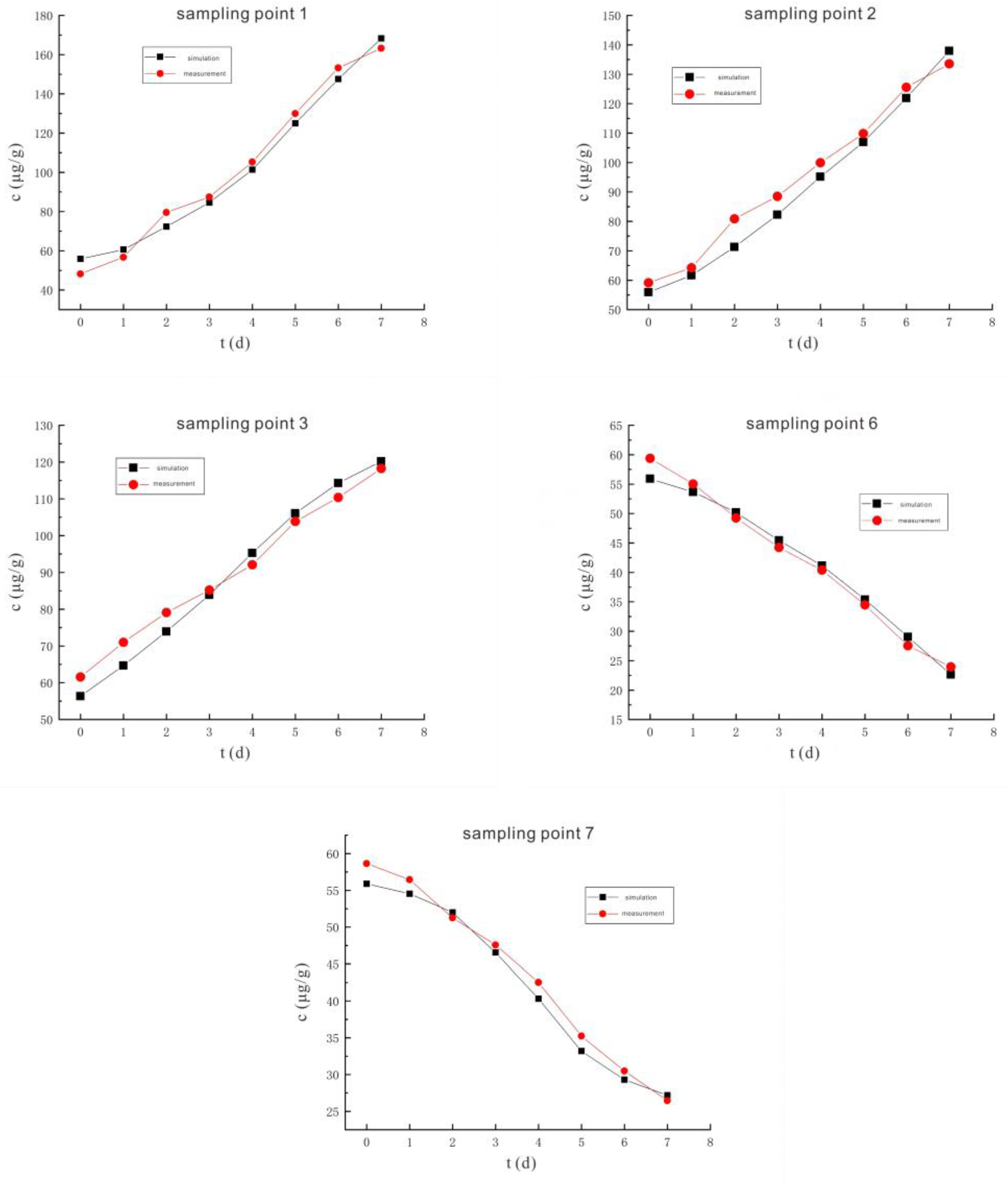
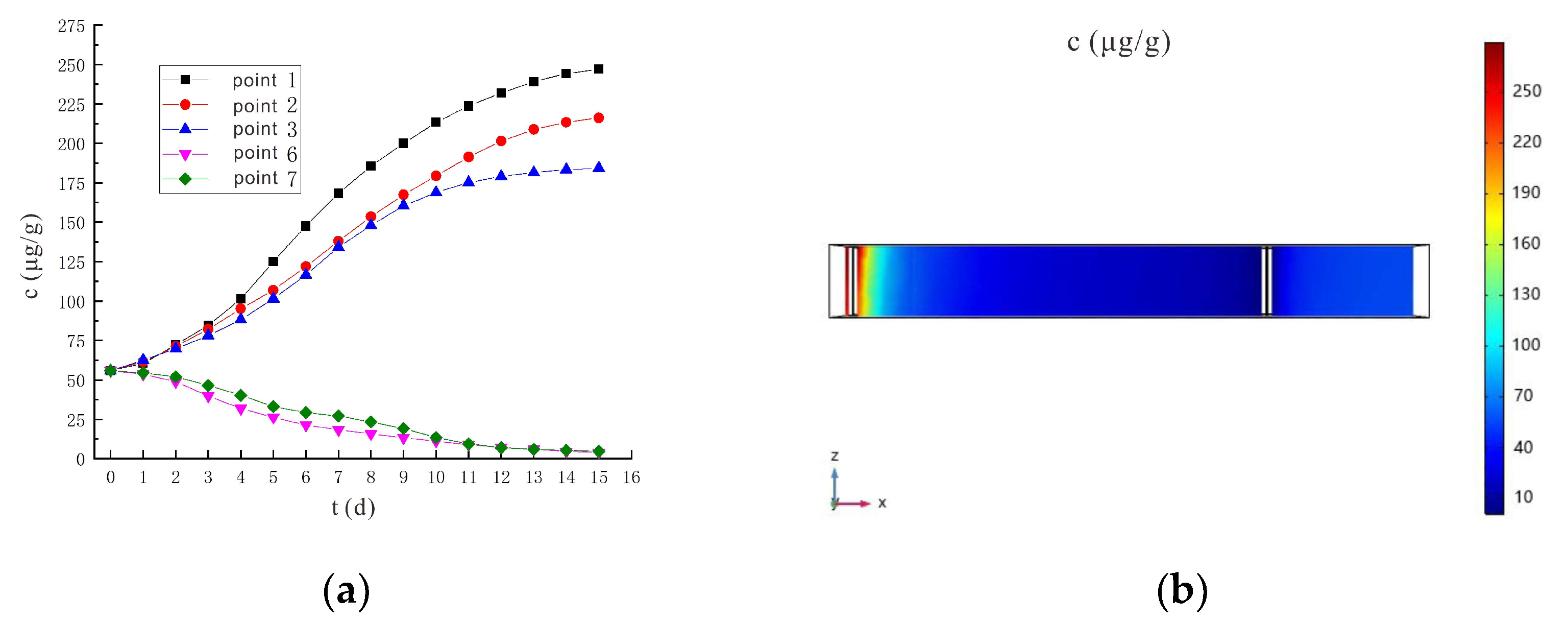
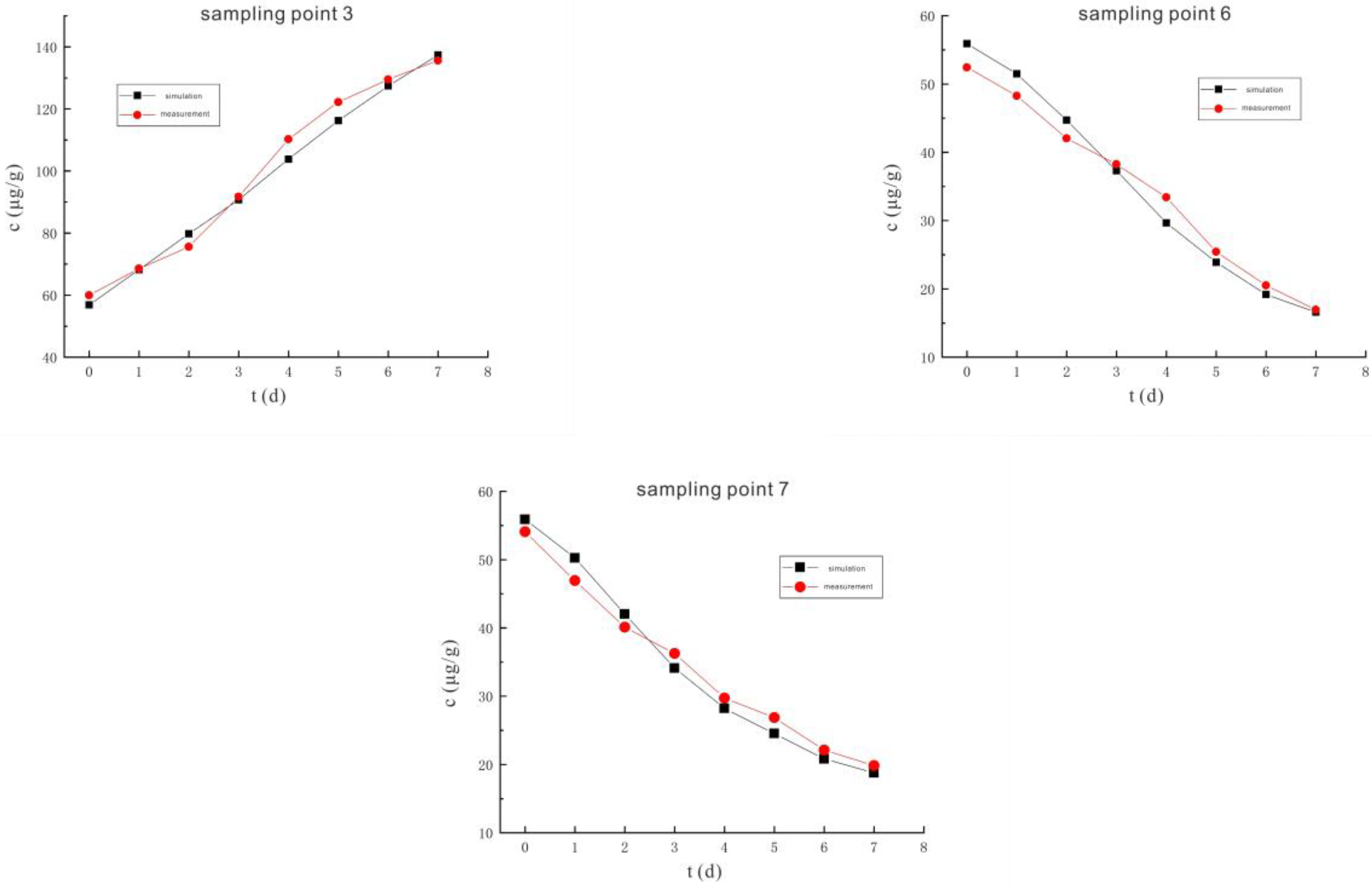
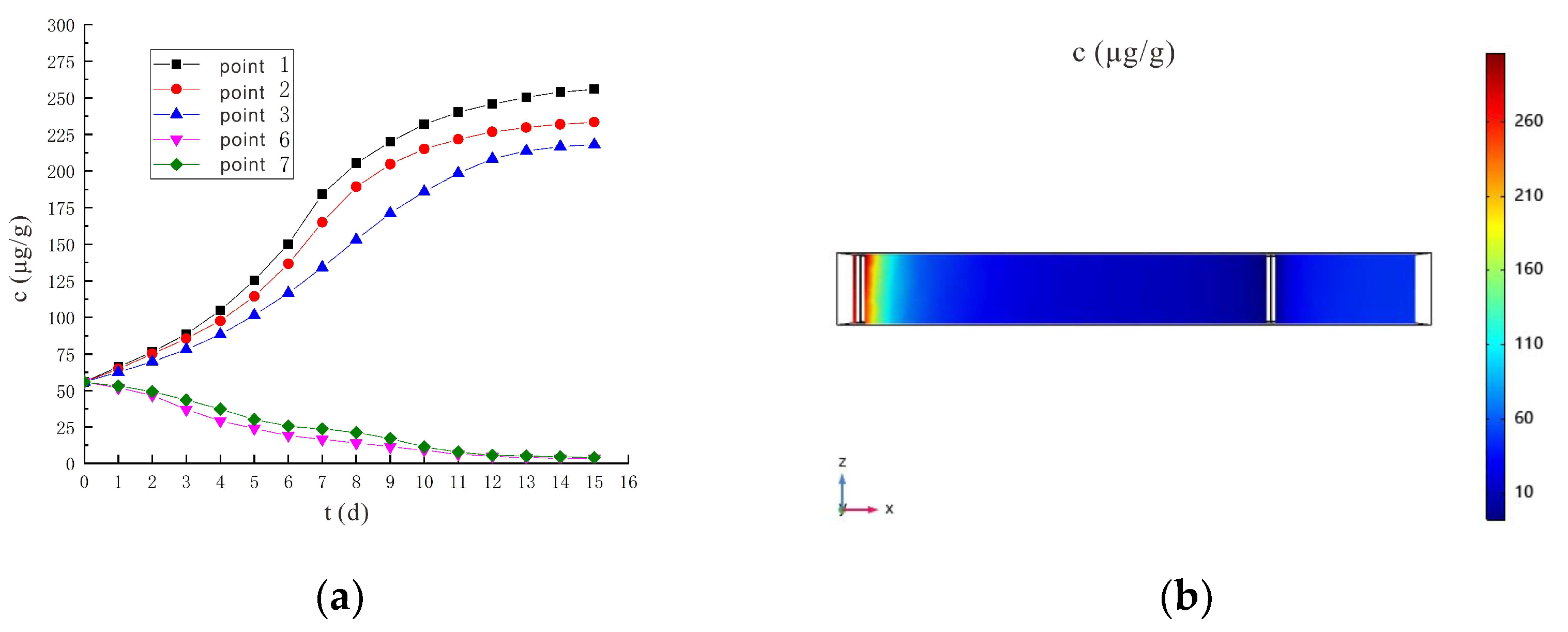
3.3. Variation Characteristics of Cr(VI) Concentration

3.3.1. Voltage 90 V, Electrode Distance 1.5 m

Figure 21 is the comparison curve between the measured and simulated values of the hexavalent chromium concentration at the five sampling points 1, 2, 3, 6 and 7 under the conditions of a voltage of 90 V and an electrode distance of 1.5 m. There is a certain difference between the simulated value curve and the measured value curve of hexavalent chromium concentration at each sampling point. The reason is presumed to be that the initial hexavalent chromium concentration in the soil was uniformly set to 55.9 μg/g during the simulation, and the initial hexavalent chromium concentration in the experimental soil was inconsistent at different locations. At the same time, the simulation did not consider the conversion of hexavalent chromium to trivalent chromium, and in the experiment, this conversion was also one of the factors that caused the change of hexavalent chromium concentration.

The reliability of the hexavalent chromium concentration model under the conditions of 90 V and 1.5 m is quantitatively evaluated by the evaluation indicators shown in

Table 2. Evaluation index of Cr(VI) concentration under the conditions of 90 V and 1.5 m.

Experimental Conditions	Evaluation Indicators	Sampling Point Number
		Sampling Point 1	Sampling Point 2	Sampling Point 3	Sampling Point 6	Sampling Point 7
90 V, 1.5 m	RMSE	5.38	5.15	4.02	1.65	1.73
	R2	0.94	0.96	0.98	0.99	0.99
	NSE	0.94	0.90	0.80	0.63	0.98

. It can be found that the two indicators of R² and NSE indicate that the similarity between the simulated value and the measured value is strong, while the RMSE indicator is on the high side. Combining these three indicators, this study believes that the model is generally trustworthy, but there are certain errors.

The predicted graph of hexavalent chromium concentration under the conditions of 90 V and 1.5 m is shown in Figure 22a. The concentration of hexavalent chromium in sampling points 6 and 7 continues to decrease during the 15th day, and drop to 4.63 μg/g and 5.29 μg/g, respectively, on the 14th day, which is lower than the soil hexavalent chromium risk control value of 5.7 μg/g. The concentration of hexavalent chromium meets the repair requirements. Figure 22b shows the distribution of Cr(VI) concentration on the 14th day under the conditions of 90 V and 1.5 m. At this point, the remediation requirements have been met, and the contaminants are mainly concentrated near the anode.

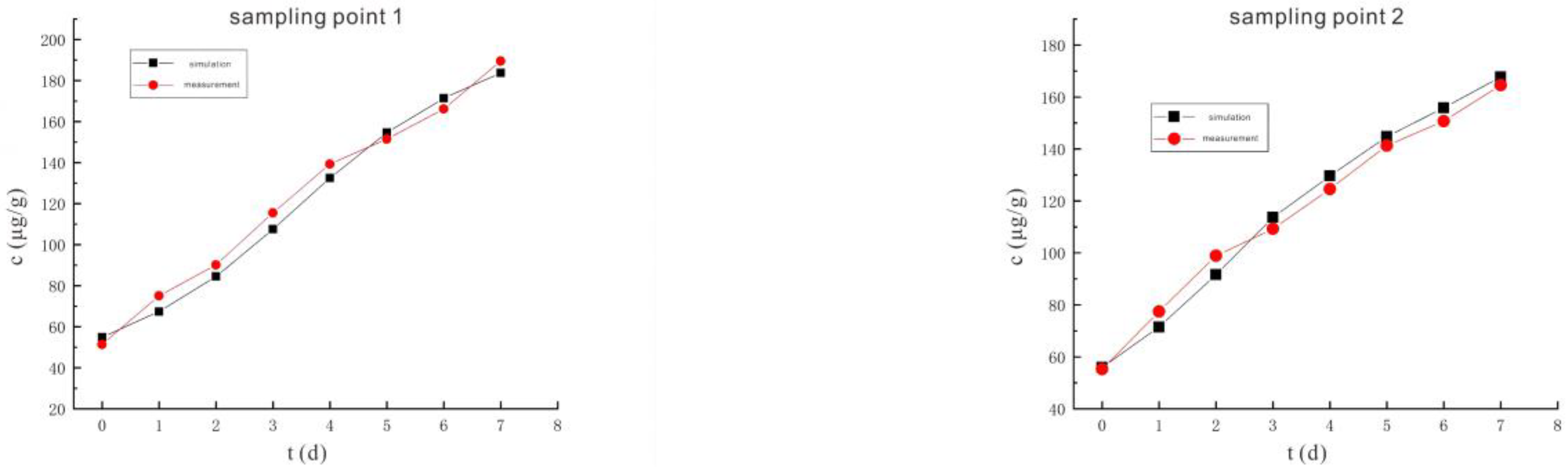
3.3.2. Voltage 110 V, Electrode Distance 1.5 m

Figure 23 is the comparison curve between the measured and simulated values of the hexavalent chromium concentration at five sampling points 1, 2, 3, 6, and 7 under the conditions of a voltage of 110 V and an electrode distance of 1.5 m. The change trend of the hexavalent chromium concentration curve of each sampling point is similar to that of 90 V, and the reason is the same as that of the voltage of 90 V.

The reliability of the hexavalent chromium concentration model under the conditions of 110 V and 1.5 m is quantitatively evaluated by the evaluation indicators shown in

Table 3. Evaluation index of hexavalent chromium concentration under the conditions of 110 V and 1.5 m.

Experimental Conditions	Evaluation Indicators	Sampling Point Number
		Sampling Point 1	Sampling Point 2	Sampling Point 3	Sampling Point 6	Sampling Point 7
110 V, 1.5 m	RMSE	5.97	4.78	3.76	2.46	2.03
	R2	0.90	0.95	0.93	0.98	0.96
	NSE	0.79	0.65	0.77	0.94	0.82

. The two indicators of R² and NSE indicate that the similarity between the simulated value and the measured value is strong, while the RMSE indicator is high. Combining these three indicators, this study believes that the model is generally trustworthy, but there are certain errors.

Figure 24a shows the predicted hexavalent chromium concentration under the conditions of 110 V and 1.5 m. The hexavalent chromium concentration of sampling point 6 and sampling point 7 continues to decrease between 15 days, and drop to 4.75 μg/g and 5.63 μg/g respectively on the 11th day, which is lower than the soil hexavalent chromium risk control value of 5.7 μg/g and meets the remediation requirements. Figure 24b shows the distribution of Cr(VI) concentration on the 11th day under the conditions of 110 V and 1.5 m. At this point, the remediation requirements have been met, and the contaminants are mainly concentrated near the anode.

Comparing Figure 22a and Figure 24a, it can be seen that the time required for soil hexavalent chromium to meet the remediation requirements under the conditions of 110 V and 1.5 m is shorter than that under the conditions of 90 V and 1.5 m.

4. Conclusions

Through indoor experiments and the establishment of an electric repair model, the following conclusions are drawn:

(1)

During the electrification process of the indoor experiment of electric remediation, the volumetric water content of the soil near the anode began to decline. After the external supplementary water arrived, the volumetric water content of the soil near the anode gradually increased. As the voltage increases, the soil volumetric water content decreases to a greater extent. The electrolysis of water occurs in a certain range near the anode and cathode electrodes, and this range will expand when the voltage increases. Beyond this range, the influence of the electric field on the water transport can be ignored.

(2)

The closer the location to the cathode or anode, the faster the rate of soil temperature rise and the higher the maximum temperature that can be reached. Furthermore, the higher the voltage, the faster the soil temperature rises at the same location and the higher the peak temperature that can be reached. At a voltage of 90 V and an electrode distance of 1.5 m, the maximum temperature can reach 36.9 °C at a distance of 5 cm from the anode. At 110 V and an electrode distance of 1.5 m, the maximum temperature can reach 52.4 °C at a distance of 5 cm from the anode. The higher temperature also contributes to soil moisture transport.

(3)

An increase in voltage would increase the removal rate of Cr(VI), and the removal rate of Cr(VI) was higher in shallow soil than in deep soil. After 7 days of electrokinetic remediation, the Cr(VI) removal rates reached 66.03% and 60.80% for sampling points 6 and 7, respectively, at a voltage of 90 V and an electrode distance of 1.5 m. In particular, at 110 V and 1.5 m electrode distance, the removal rates of Cr(VI) at sampling points 6 and 7 reached 75.96% and 70.74%, respectively. The removal rate was improved by nearly 10% at higher voltage conditions.

(4)

Through the numerical simulation prediction results of the soil volumetric water content at different depths in the same location, it is found that the soil volumetric water content at the shallower depths is initially greater than that at the deeper depths. However, with the increase of time, the gap between the two will gradually narrow, and finally the volumetric water content of the soil at the deeper depths will in turn exceed the volumetric water content of the soil at the shallower depths.

(5)

It is predicted by numerical simulation that under the conditions of a voltage of 90 V and an electrode distance of 1.5 m, the content of hexavalent chromium in the soil at the sampling point on the 14th day is lower than the risk control value of hexavalent chromium in the soil 5.7 μg/g, which meets the remediation requirements. Under the conditions of a voltage of 110 V and an electrode distance of 1.5 m, the soil at the sampling point met the remediation requirements after 11 days. The increased voltage shortens the time it takes for the soil remediation to succeed.

(6)

This study did not consider the conversion of hexavalent chromium to trivalent chromium, which is also an important factor in the change of hexavalent chromium content in soil, so future work could be improved; at the same time, the influence of evaporation conditions was missing in the modeling process, and there was a relatively large increase in soil temperature under the action of the electric field, which would cause the strengthening of evaporation, and this factor would have some influence on the volumetric water content of soil. Additionally, the possible influence of electric remediation on the soil ecosystem of contaminated sites also needs to be included in future consideration.

References

1. Yin, Z.; Zhang, J.C.; Liao, S.L.; Ma, Q.; Wang, Q.G.; Zhang, J.F. Research and Application of Remediation Technology for Chromium Contaminated Sites. Environ. Eng. 2015, 33, 159–162. [Google Scholar]
2. Kotas, J.; Stasicka, Z. Chromium occurrence in the environment and methods of its speciation. Environ. Pollut. 2000, 107, 263–283. [Google Scholar] [CrossRef]
3. Hu, L.G.; Cai, Y.; Jiang, G.B. Occurrence and speciation of polymeric chromium(III), monomeric chromium(III) and chromium(VI) in environmental samples. Chemosphere 2016, 156, 14–20. [Google Scholar] [CrossRef] [Green Version]
4. Xu, R.; Wang, H.; Sun, Y.; Gao, Y.; Li, S.; Wang, Y.; Guo, L. Remediation of Cr(VI) from contaminated soil with the combination of biogas residue and ferrous sulfate. Acta Sci. Circumstantiae 2021, 41, 4161–4169. [Google Scholar]
5. Sarangi, A.; Krishnan, C. Comparison of in vitro Cr(VI) reduction by CFEs of chromate resistant bacteria isolated from chromate contaminated soil. Bioresour. Technol. 2008, 99, 4130–4137. [Google Scholar] [CrossRef]
6. Deng, H.; Chen, G. Progress in Research on Microbial Remediation Technologies of Chromium-Contaminated Soil. Earth Environ. 2012, 40, 466–472. [Google Scholar]
7. Li, J.; Huang, J. Studies and prospect on the speciation analysis of chromium. Metall. Anal. 2006, 26, 38–43. [Google Scholar]
8. Wang, W.; Liu, Y.; Huang, S.; Li, Y.; Zhou, L.; Cheng, J. Stabilization of Cr(VI)-contaminated soil with calcium polysulfide. Chin. J. Environ. Eng. 2017, 11, 3853–3860. [Google Scholar]
9. Shahid, M.; Shamshad, S.; Rafiq, M.; Khalid, S.; Bibi, I.; Niazi, N.K.; Dumat, C.; Rashid, M.I. Chromium speciation, bioavailability, uptake, toxicity and detoxification in soil-plant system: A review. Chemosphere 2017, 178, 513–533. [Google Scholar] [CrossRef]
10. Setshedi, K.Z.; Bhaumik, M.; Onyango, M.S.; Maity, A. Breakthrough studies for Cr(VI) sorption from aqueous solution using exfoliated polypyrrole-organically modified montmorillonite clay nanocomposite. J. Ind. Eng. Chem. 2014, 20, 2208–2216. [Google Scholar] [CrossRef]
11. Hutchison, J.M.; Seaman, J.C.; Aburime, S.A.; Radcliffe, D.E. Chromate Transport and Retention in Variably Saturated Soil Columns. Vadose Zone J. 2003, 2, 702–714. [Google Scholar] [CrossRef]
12. Wang, X.R.; Li, L.; Yan, X.H.; Tian, Y.Q. Progress in remediation of chromium-contaminated sites. Environ. Eng. 2020, 38, 1–8. [Google Scholar]
13. Zhang, X.Y.; Zhong, T.Y.; Liu, L.; Zhang, X.M.; Cheng, M.; Li, X.H.; Jin, J.X. Chromium occurrences in arable soil and its influence on food production in China. Environ. Earth Sci. 2016, 75, 257. [Google Scholar] [CrossRef]
14. Zhang, Q.C.; Wang, C.C. Natural and Human Factors Affect the Distribution of Soil Heavy Metal Pollution: A Review. Water Air Soil Pollut. 2020, 231, 350. [Google Scholar] [CrossRef]
15. Ertani, A.; Mietto, A.; Borin, M.; Nardi, S. Chromium in Agricultural Soils and Crops: A Review. Water Air Soil Pollut. 2017, 228, 190. [Google Scholar] [CrossRef]
16. Liu, Y.; Su, C.; Zhang, H.; Li, X.T.; Pei, J.F. Interaction of Soil Heavy Metal Pollution with Industrialisation and the Landscape Pattern in Taiyuan City, China. PLoS ONE 2014, 9, e105798. [Google Scholar] [CrossRef]
17. Li, C.; Li, F.B.; Wu, Z.F.; Cheng, J. Impacts of landscape patterns on heavy metal contamination of agricultural top soils in the Pearl River Delta, South China. Chin. J. Appl. Ecol. 2015, 26, 1137–1144. [Google Scholar]
18. Jeon, E.K.; Ryu, S.R.; Baek, K. Application of solar-cells in the electrokinetic remediation of As-contaminated soil. Electrochim. Acta 2015, 181, 160–166. [Google Scholar] [CrossRef]
19. Ribeiro, A.; Mota, A.; Soares, M.; Castro, C.; Araújo, J.; Carvalho, J. Lead (II) Removal from Contaminated Soils by Electrokinetic Remediation Coupled with Modified Eggshell Waste. Key Eng. Mater. 2018, 777, 256–261. [Google Scholar] [CrossRef]
20. Ortiz-Soto, R.; Leal, D.; Gutierrez, C.; Aracena, A.; Rojo, A.; Hansen, H.K. Electrokinetic remediation of manganese and zinc in copper mine tailings. J. Hazard. Mater. 2019, 365, 905–911. [Google Scholar] [CrossRef]
21. Li, M.; Sun, Z.; Ma, C.; Yao, X. Electrochemical combined remediation of chromium contaminated soil based on strengthening by anode consumption. Environ. Eng. 2020, 38, 224–230. [Google Scholar]
22. Tang, J.; Qiu, Z.P.; Tang, H.J.; Wang, H.Y.; Sima, W.P.; Liang, C.; Liao, Y.; Li, Z.H.; Wan, S.; Dong, J.W. Coupled with EDDS and approaching anode technique enhanced electrokinetic remediation removal heavy metal from sludge. Environ. Pollut. 2021, 272, 115975. [Google Scholar] [CrossRef] [PubMed]
23. Telepanich, A.; Marshall, T.; Gregori, S.; Marangoni, A.G.; Pensini, E. Graphene-Alginate Fluids as Unconventional Electrodes for the Electrokinetic Remediation of Cr(VI). Water Air Soil Pollut. 2021, 232, 334. [Google Scholar] [CrossRef]
24. Xu, H.C.; Bai, J.; Yang, X.R.; Zhang, C.P.; Yao, M.; Zhao, Y.S. Lab scale-study on the efficiency and distribution of energy consumption in chromium contaminated aquifer electrokinetic remediation. Environ. Technol. Innov. 2022, 25, 102194. [Google Scholar] [CrossRef]
25. Wang, Y.C.; Han, Z.J.; Li, A.; Cui, C.W. Enhanced electrokinetic remediation of heavy metals contaminated soil by biodegradable complexing agents. Environ. Pollut. 2021, 283, 117111. [Google Scholar] [CrossRef]
26. Rezaee, M.; Asadollahfardi, G. An Implicit Finite Difference Model for Electrokinetic Remediation of Cd-Spiked Kaolinite Under Acid-Enhanced and Unenhanced Conditions. Environ. Model. Assess. 2019, 24, 235–248. [Google Scholar] [CrossRef]
27. Lopez-Vizcaino, R.; Yustres, A.; Leon, M.J.; Saez, C.; Canizares, P.; Rodrigo, M.A.; Navarro, V. Multiphysics Implementation of Electrokinetic Remediation Models for Natural Soils and Porewaters. Electrochim. Acta 2017, 225, 93–104. [Google Scholar] [CrossRef]
28. Alshwabkeh, A.N.; Acar, Y.B. Electrokinetic Remediation II: Theoretical Mode. J. Geotech. Eng. 1996, 122, 186–196. [Google Scholar] [CrossRef]
29. Wang, Z.; Gu, X.; Xie, T.; Xu, X. Simulation of Heavy Metal Pollutants Migration in Soil Based on Finite Volume Method. J. Northeast. Univ. Nat. Sci. 2018, 39, 867–871. [Google Scholar]
30. Liu, X.M.; Ma, C.; Tao, J.X.; Tian, B.R. Diphenylcarbohydrazide spectrophotometry and its improved methods for the determination of chromium(Ⅵ). Appl. Chem. Ind. 2018, 47, 1308–1311. [Google Scholar]
31. Tang, T.; Wang, Y.; Tang, H.; Ren, J. Determination of hexavalent chromium in soil. Sichuan Environ. 2017, 36, 123–126. [Google Scholar]
32. Xu, Y.B.; Fan, X.J.; Gong, X. Improvement of Spectrophotometric Determination of Hexavalent Chromium in Water with Diphenylcarbazide. China Water Wastewater 2015, 31, 106–108. [Google Scholar]
33. Pourmohammad, M.; Faraji, M.; Jafarinejad, S. Extraction of chromium (VI) in water samples by dispersive liquid-liquid microextraction based on deep eutectic solvent and determination by UV-Vis spectrophotometry. Int. J. Environ. Anal. Chem. 2020, 100, 1146–1159. [Google Scholar] [CrossRef]
34. Leng, Y.P.; Xue, X.K.; Zhang, M.H. Chromium reduction of hexavalent chromium detected by soil alkaline digestion and analysis of quality control results. J. Anhui Agric. Sci. 2019, 47, 206–208. [Google Scholar]
35. Ma, W.; Zhou, Q.; Zhu, L.Z.; Wang, L.; Ji, Y.J. Study on Determination of Hexavalent Chromium in Solid Waste by Alkaline Digestion. Environ. Prot. Sci. 2012, 38, 41–43. [Google Scholar]
36. Yi, M.; Ou, F.P. Rapid pretreatment method for alkali digestion of solid waste hexavalent chromium analytical samples. Environ. Eng. 2010, 28, 87–88. [Google Scholar]
37. Qin, T.; Dong, Z.F.; Lv, X.H.; Zhang, X.L. Determination of Hexavalent Chromium in Soil by Alkaline Digestion-Inductively Coupled Plasma Optical Emission Spectroscopy (ICP-OES). Chin. J. Inorg. Anal. Chem. 2019, 9, 10–13. [Google Scholar]
38. Huang, J.; Huang, Y.; Yao, J.; Wang, C.X. Determination of Hexavalent Chromium in PM10 by Alkaline Digestion-Graphite Furnace Atomic Absorption Spectrometry. Chem. Anal. Meterage 2015, 24, 52–54. [Google Scholar]
39. Chen, X.L.; Wang, Y.M.; Zhao, Y.K.; Li, Z.Y.; Yi, B.Z.; Xu, L.; Sha, J.; Huang, Y. Comparison and Research of Acid Digestion Technique for Pt, Pd and Rh in Catalysts. Rare Met. Mater. Eng. 2011, 40, 1867–1870. [Google Scholar]
40. Li, Q.; Cao, Y.; Gao, C.; Liu, Y.; Zhou, M.; Liu, X. Comparative study of acidification systems for determination of heavy metals in soils from different areas in China. Environ. Chem. 2020, 39, 1153–1157. [Google Scholar]
41. Li, R.; Wu, B.; Wang, S.; Li, G. Analysis of key parameters for electrokinetic remediation of contaminated soil under high electric field strength. Environ. Eng. 2018, 36, 149–153. [Google Scholar]
Figure 1. Experimental setup.
Sustainability 14 08136 g001
Figure 2. Layout of observation points. (a) Top view; (b) Left view; (c) Main view; (d) Sectional view.
Sustainability 14 08136 g002aSustainability 14 08136 g002b
Figure 3. Cr(VI) standard curve.
Sustainability 14 08136 g003
Figure 4. 3D geometric model.
Sustainability 14 08136 g004
Figure 5. Location map of each observation point.
Sustainability 14 08136 g005
Figure 6. Meshing diagram of the electric repair model.
Sustainability 14 08136 g006
Figure 7. Variation trend of soil volumetric water content under the conditions of 90 V and 1.5 m. (a) Moisture monitoring points a~d; (b) Moisture monitoring points e~h.
Sustainability 14 08136 g007
Figure 8. Variation trend of soil volumetric water content under the conditions of 110 V and 1.5 m. (a) Moisture monitoring points a~d; (b) Moisture monitoring points e~h.
Sustainability 14 08136 g008
Figure 9. Changes of soil temperature at each monitoring point under the conditions of voltage 90 V and electrode distance of 1.5 m, a~h are the temperature monitoring points.
Sustainability 14 08136 g009
Figure 10. Changes in soil temperature at each monitoring point under the conditions of voltage 110 V and electrode distance of 1.5 m, a~h are the temperature monitoring points.
Sustainability 14 08136 g010
Figure 11. Change of Cr(VI) concentration under the conditions of voltage of 90 V and electrode distance of 1.5 m. (a) Concentration monitoring points 1~5; (b) Concentration monitoring points 6~10.
Sustainability 14 08136 g011
Figure 12. Changes of Cr(VI) concentration under the conditions of voltage 110 V and electrode distance of 1.5 m. (a) Concentration monitoring points 1~5; (b) Concentration monitoring points 6~10.
Sustainability 14 08136 g012
Figure 13. Cloud map of moisture distribution under the conditions of 90 V and 1.5 m for 7 days (168 h).
Sustainability 14 08136 g013aSustainability 14 08136 g013bSustainability 14 08136 g013c
Figure 14. The comparison curve between the measured value and the simulated value of soil volumetric water content under the conditions of 90 V and 1.5 m.
Sustainability 14 08136 g014aSustainability 14 08136 g014b
Figure 15. Simulation results and evaluation indexes of soil volumetric water content under the conditions of 90 V and 1.5 m.
Sustainability 14 08136 g015
Figure 16. Moisture prediction diagram under the conditions of 90 V and 1.5 m, a~h are the moisture monitoring points.
Sustainability 14 08136 g016
Figure 17. Cloud map of moisture distribution under the conditions of 110 V and 1.5 m for 7 days (168 h).
Sustainability 14 08136 g017aSustainability 14 08136 g017bSustainability 14 08136 g017c
Figure 18. The comparison curve between the measured value and the simulated value of soil volumetric water content under the conditions of 110 V and 1.5 m.
Sustainability 14 08136 g018aSustainability 14 08136 g018b
Figure 19. Simulation results and evaluation indicators of soil volumetric water content under the conditions of 110 V and 1.5 m.
Sustainability 14 08136 g019aSustainability 14 08136 g019b
Figure 20. Prediction of moisture content under the conditions of 110 V and 1.5 m, a~h are the moisture monitoring points.
Sustainability 14 08136 g020
Figure 21. The comparison curve between the measured and simulated values of hexavalent chromium concentration under the conditions of 90 V and 1.5 m.
Sustainability 14 08136 g021
Figure 22. (a) Prediction chart of hexavalent chromium concentration under the conditions of 90 V and 1.5 m; (b) Cr(VI) concentration distribution on day 14.
Sustainability 14 08136 g022
Figure 23. The comparison curve between the measured value and the simulated value of hexavalent chromium concentration under the conditions of 110 V and 1.5 m.
Sustainability 14 08136 g023aSustainability 14 08136 g023b
Figure 24. (a) Prediction chart of hexavalent chromium concentration under the conditions of 110 V and 1.5 m; (b) Cr(VI) concentration distribution on day 11.
Sustainability 14 08136 g024