Article

Large Scale Energy Signature Analysis: Tools for Utility Managers and Planners

1
Department of Building Research, Korea Institute of Civil Engineering and Building Technology, Goyang-si 10223, Korea
2
Mechanical and Biomedical Engineering, Boise State University, 1910 University Drive, Boise, ID 83725, USA
*
Author to whom correspondence should be addressed.
Sustainability 2022, 14(14), 8649; https://doi.org/10.3390/su14148649
Submission received: 3 May 2022 / Revised: 30 June 2022 / Accepted: 11 July 2022 / Published: 14 July 2022

Abstract

:
Building energy signature analysis is a well-established tool for understanding the temperature sensitivity of building energy consumption and measuring energy savings. This tool has been used to measure energy savings of residential, commercial, and even industrial buildings. The public availability of electricity loads (i.e., hourly electricity demand (MW)) from entire Balancing Authorities (BAs) provide an interesting opportunity to apply this approach to a large aggregate load. In this paper, we explore that opportunity for BAs and show that the correlations for large geographical areas are surprisingly coherent when the change-point linear regression analysis is used with the daily interval data of electricity demand and outside air temperature. The change-point linear regression models of all the BAs, except WAUW and OVEC, show R2 of 0.70 or more and CV-RMSE of 10.0% or less. We also suggest an analysis method that allows for meaningful comparisons between BAs and to assess changes in time for a given BA which could be used to interpret changes in load patterns year-to-year, accounting for changes in weather. This approach can be used to verify the impact of energy efficiency programs on a building component/system-wide basis. This study shows the annual electricity demand reductions for SCL and IPCO are 136,655 MWh (1.5%) and 182,053 MWh (1.1%), respectively.

1. Introduction

Utility companies and non-utility organizations have operated energy efficiency programs to reduce energy use, economic cost, and greenhouse gases [1]. Energy efficiency programs generally include rebates and incentives for customers when they buy energy efficient products. Weatherization is also offered for low-income houses [2,3]. Recently, new technologies, exemplified by the advanced metering infrastructure, can affect the energy efficiency programs because the new technologies provide interactive information for utilities and customers [4,5].
Over the last three decades, energy efficiency programs have emerged as a crucial strategy for meeting new demands and decreasing carbon emissions from the energy sector [5,6]. As these programs evolve, the challenge of the valuation of these programs continues to be a complex problem, including a range of characteristics from the measurement and verification of actual energy savings to the value of those savings for the utility and the consumer [5]. In addition, examining how well energy efficiency programs and policies provide improvements in energy efficiency is also important [7].
Building energy signature analysis is a well-established tool for assessing energy savings from buildings. Such tools have been used to analyze residential, commercial, and even industrial buildings [8,9,10]. Energy signature analysis is a data-driven or inverse modeling method. The analysis is steady-state in nature, making use of energy consumption summed over time periods which normally exclude the energy dynamics brought about by the building thermal mass. Typical time intervals for the data range from hourly (which can contain dynamic response data) to monthly, corresponding to typical utility billing periods. This approach also requires coincident weather data. Single-variate inverse modeling using one independent variable of outside air temperature is popular because this approach is simple and reliable [9,11,12].
The change-point or piece-wise linear regression models are used for individual loads or used extensively for aggregate loads or regional datasets from individual loads. Raffio et al. examined three-parameter (3P) heating and cooling change-point models for individual monthly utility billing data from 260 residences in Dayton, Ohio [13]. They analyzed the parameters of the models and identified why abnormal coefficients occurred by visiting the selected houses. Perez et al. used a 3P cooling change-point model for daily air conditioning (AC) systems from 45 houses in Austin, Texas [8]. They compared the cooling slopes of each 3P model, which can be used to identify houses worthy of targeting for energy efficiency improvements. In addition, Gianniou et al. used an Ordinary Least Squares (OLS) method, which is similar to a 3P heating change-point model, for hourly heating loads from about 14,000 households in Aarhus, Denmark [14]. They estimated and compared inside temperature setpoints and total heat loss coefficients obtained from the large amount of individual heating load data. Eriksson et al. used a 3P heating change-point model to estimate the heating energy use of 95 multi-family buildings in a Swedish city district [15]. The researchers accounted for the heat loss coefficient, heating balance-point temperature, domestic hot water demand, and domestic hot water circulation demand. The district heating demands before and after the building renovation were compared using hourly interval data, and the heating energy signature was identified. Ding et al. used piece-wise or 4P heating change-point models using hourly interval data for weekdays and weekends to analyze electric heating use in educational and residential buildings in Norway [16]. Using the 4P models, the researchers established new energy signature curves based on the scenarios considering the COVID-19 situations, and then analyzed the electricity demand by the building types and the scenarios. Aragon et al. also examined piece-wise or 4P heating change-point models to evaluate the weekly heat demand of 462 dwellings in the south of the UK [17]. They analyzed the various energy trends of the social housing dwellings such as the houses that do not require space heating or show irregular heating use, as well as the houses that demonstrate no variation or no additional heating energy use when extreme weather events occurred.
Even though the change-point linear regression analysis has been widely used in the previous studies [8,9,10,13,14,15,16,17], few previous studies have provided the analysis of aggregate loads by different region using this change-point approach. Although many researchers use this approach of multiple loads for comparison or planning purposes, there are few instances of attempting to use this approach for a large number of loads in aggregate. One example is found in Ali et al. [18], where they developed a 3P cooling change-point model for daily aggregate cooling load from about 800,000 residential and commercial buildings in Abu Dhabi, United Arab Emirates, but they used additional humidity and solar irradiation terms for the model to predict cooling loads and the results were used as a predictive and planning tool. Finally, Wang et al. [19] examined the Balancing Authorities (BAs) data that were also used in this study. However, they focused on comparing data-driven models using the data from three BAs rather than utilizing the results from the change-point linear regression analysis.
In summary, all the previous studies did not suggest energy analysis methods using the simple datasets of energy use and outside air temperature for the aggregate loads in large areas to characterize energy patterns and to identify energy saving opportunities. The public availability of electric loads (from the EIA-930 survey) for entire Balancing Authorities (BAs) [20,21] (now called the Hourly Electric Grid Monitor [22]) provide an interesting opportunity to apply the change-point linear regression method to a large aggregate load (i.e., grid-level electricity use). BAs control electric generation and transmission to maintain the balance of their areas. Each BA ensures electricity supply to meet expected demand and manages transfers with other BAs. The quality of the data from BAs has been well controlled [23]. In this paper, we explore that opportunity and show that the correlations for large geographical areas (e.g., BA region) are surprisingly coherent when the change-point linear regression analysis is used. This is important because the change-point models have been widely used because of the simplicity and the reliability. Even when the change-point linear regression analysis is compared with the degree day method [24], the change-point linear regression analysis shows better usability and accuracy [19]. The tools using the change-point models will be very useful for utility managers and planners because the electricity demand in large areas can be easily characterized using outside air temperature data only (i.e., large scale energy signature analysis). In addition, we suggest a weather-adjusted analysis method (i.e., another easy-to-use analysis tool) that will allow for meaningful comparisons between BAs and to assess changes in time for a given BA based on energy efficiency programs that are searched for each BA. These show the novelty of this study that provides the easy-to-use and the easy-to-interpret tools for the energy demand and the energy savings of large areas in order to identify energy signature, including weather-dependent and weather-independent energy demand and savings. The next section describes the datasets and the methods used in this study. Section 3 presents the results from the energy signature analysis using the change-point linear regression models and the results from the weather-adjusted method. Then, the discussion and the conclusions of this study are presented in Section 4 and Section 5, respectively.

2. Materials and Methods

2.1. Electricity Demand Data

EIA-930 datasets (now called the Hourly Electric Grid Monitor) that include hourly electricity demand (MW) for each BA are compiled by US Energy Information Administration (EIA) [25]. The EIA portal supports the monitoring tool that analyzes and visualizes the electricity data on a national and regional level for all 68 BAs [20,22,25]. The data can also be downloaded in a machine-readable file with the first entries beginning in July 2015. The data for each BA generally includes interval data for actual demand, day-ahead predicted demand, net generation, and interchange data between BAs. Errors and discrepancies encountered in compiling these data are addressed in the report [26].

2.2. Selected BA

In total, 14 BAs were selected to examine how well the energy signature analysis works. Figure 1 shows the 14 BAs selected for this paper. For further analysis, four BAs (highlighted by red) are compared with two different annual periods to track changes in the load characteristics over time, which could be a result of their energy efficiency programs.
Table 1 shows a list of the selected 14 BAs. They comprise a sample of geographically compact BAs, which are more likely to occur in the Pacific Northwest, as well more dispersed BAs, such as MISO. In this study, the BAs that cover smaller areas and are located in the Pacific Northwest are selected first to reduce the uncertainty from the types of buildings/people, as well as the types of industry that the BAs service. The next level of this study will include the analysis using knowledge-based databases, including surveys of demographics, industry types, etc. For reference, the International Energy Conservation Code (IECC) climate zones [29] are compared in Table 1. A higher number means that the region has more heating degree days (i.e., colder climate). A, B, and C represent moist, dry, and marine conditions, respectively. For example, SCL and TPWR are in the mild and marine climate, and HST is in the hot and dry climate.
Outside air temperature data were collected from a NOAA reporting station [30] deemed to be representative of each BA. For example, IPCO covers an area from Eastern Oregon to the Wyoming border across southern Idaho. However, most customers in IPCO are located in Boise, ID, so the temperature data from the Boise reporting station was used. It is noted that the same NOAA weather data is used for SCL(4C), TPWR(4C), and PSEI(5B) because the service areas of the BAs are placed in the marine climate.
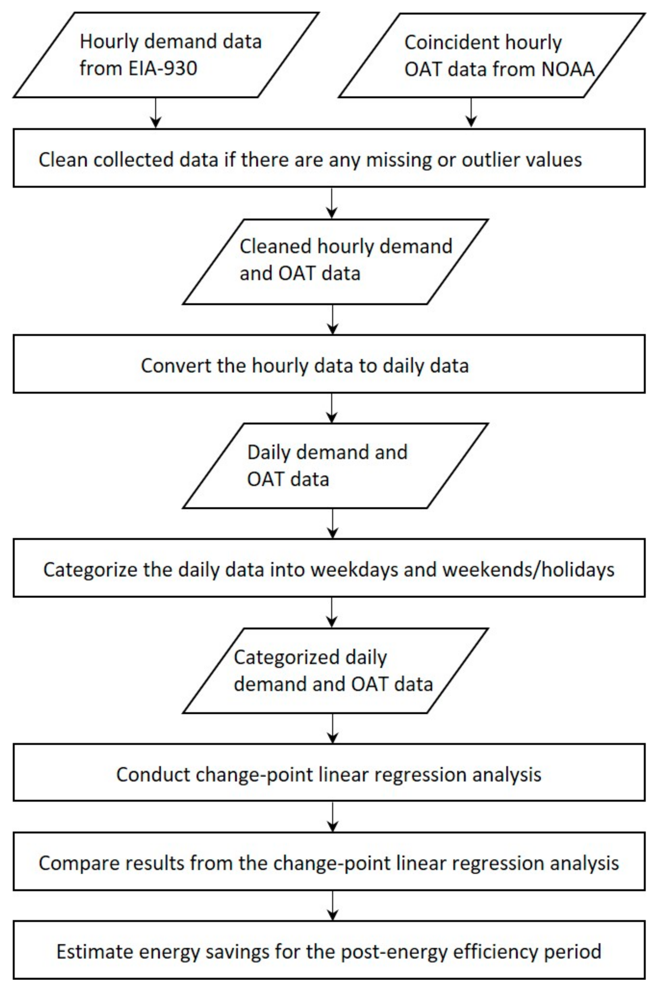
Of the 14 BAs, the four BAs of SCL, IPCO, IID, and HST were selected for comparison with the two different annual periods using a weather-adjusted method in an attempt to examine changes over time and to correct for different weather patterns. The overall methodology of this study is shown in Figure 2. The major steps of the methodology are summarized below:
-
Hourly interval electricity demand data (MW) for 14 BAs were collected for the one-year period from January 2016 to December 2016. For further analysis, hourly interval electricity demand data (MW) for four BAs were collected for the two periods: July 2015 to June 2016 and July 2017 to June 2018. In addition, the corresponding hourly outside air temperature (OAT) (°C) data were collected for each BA [30];
-
Blank, zero, and minus values from hourly electricity demand data were considered as missing values. Outliers were then removed for hourly electricity demand data. If hourly demand was above two times of the maximum value and below the half of the minimum value during the year, the hourly demand was considered as an outlier. When missing and outlier data exist in a day for hourly electricity demand data, the day was handled as a missing and outlier day, respectively. In addition, missing data were filled in for the hourly outside air temperature data using a linear interpolation method when missing data were found [31];
-
Hourly data were converted to daily data. The hourly demand data were added and the hourly OAT data were averaged for the daily intervals;
-
The daily data were organized by dividing the data into the two categories: weekdays (WDs) and weekends/holidays (WEs);
-
Change-point linear regression analysis was conducted using the ASHRAE Inverse Modeling Toolkit (IMT) [32] to find a balance-point temperature, a heating or cooling slope (weather-dependent electricity demand), and weather-independent electricity demand for each BA;
-
The results from the change-point analysis were compared for 14 BAs. Furthermore, four BAs were compared with two different periods, which assumed that the periods were pre- and post-energy efficiency program periods, respectively. In addition, energy savings were estimated using a weather-adjusted method [9] for four BAs during a post-energy efficiency program period.
We use change-point linear regression models [32] for energy signature analysis because the change-point models are effective, and they can examine details by weather-dependent and weather-independent demand use. We use daily interval data because we found that the models for the daily data fit well compared to the models for hourly or weekly interval data.

2.3. Model

Fundamentally, the change-point linear regression model is a curve-fitting approach which chooses the best set of parameters for the best model that fits the data [11]. The various models are differentiated by the number of parameters they use, and the parameters are slopes, temperature balance points, and the energy use that is not related to temperature. The simplest model has three parameters, one slope indicating the intensity of the temperature dependence, the level of energy use that is not temperature dependent, and the temperature at which the two regions of the model meet. This is called a three-parameter (3P) model. A 3P model indicates that the building requires either cooling or heating, but not both. A five-parameter (5P) model finds two slopes, one for both modes (heating and cooling), a balance-point temperature for each, and the level of energy use that is not related to the outside temperature, which the building consumes when the outside temperature is between the two balance-point temperatures. A variation of the 5P model is a four-parameter (4P) model in which the two balance-point temperatures are coincident. The Inverse Modeling Toolkit (IMT) [32] provides a set of computational tools that automates and regularizes the procedure of finding the best model and resulting parameters for a given dataset.
The 3P cooling and the 5P change-point linear regression models were used for the BAs in this study. The 3P cooling and 5P models can be defined mathematically as Equations (1) and (2), respectively. For the purpose of this paper, we used 24 h as the sampling interval, although other can be used to similar effect.
E t o t = E w . i . + C S ( T O A T c . b . ) +
E t o t = E w . i . + H S ( T O A T h . b . ) + C S ( T O A T c . b . ) +
where E t o t is the total BA daily electricity demand, T O A is the daily average outside air temperature (OAT) from each reporting station. The parameters for the model are: E w . i . is the daily weather-independent electricity demand, C S is the cooling slope that represents cooling electricity use sensitivity to OAT, T c . b . is the cooling balance-point (change-point) temperature, H S is the heating slope that represents heating electricity use sensitivity to OAT, and T h . b . is the heating balance-point (change-point) temperature. For the H S , absolute values were used for better visualization in the figures.
The notation (   ) + and (   ) indicate that the values of the parentheses shall be zero when they are negative and positive, respectively [32]. For example, the model described by Equation (1) ignores temperatures colder than the cooling balance-point temperature. In addition, when T h . b . is the same with the T c . b . , it makes the 4P model form for this paper.
The units of the H S and C S parameters are MWh/day/°C. Since this value is sensitive to the magnitude of the overall BA demand, a normalization is proposed which accounts for these differences and allows for comparison of the H S and C S parameters between BAs. It is assumed that the slopes and the weather independent energy parameters scale in a similar manner to the overall BA demand. Given that assumption, the slopes can be normalized by dividing by the E w . i . parameters, creating a normalized slope with the dimensions 1 °C as shown in Equations (3) and (4). For the Normalized   H S , absolute values were also used.
Normalized   H S = H S E w . i .      
Normalized   C S = C S E w . i .  
One of the more important uses of this approach is that it can be used to quantify and estimate energy savings by comparing data of two different years and account for the change in weather. This is done by using the parameters from the change-point model in the earlier year and ‘run through’ the temperature data from the later year. The results are an estimate of how aggregate load would appear if nothing other than the weather had changed. Comparing that result to the actual demand in the later year provides an estimate of the savings that could be attributed to utility programs, such as weatherization, or other efficiency measures. It should be noted that this approach assumes no substantial changes in the aggregate load due to growth or other factors. Given the relatively flat demand for electricity over the past decade, this is a reasonable assumption in some cases. This approach is shown mathematically in Equation (5) [9]:
S = i = 1 n E ^ P o s t   i E P o s t ,       m e a s u r e d   i
where S is savings from the energy efficiency program, n is the number of daily electricity demand during the post-energy efficiency program period (i.e., n = 365 or 366), E ^ P o s t   i is the total electricity demand during the post-energy efficiency program period predicted by the change-point model, and E P o s t ,   m e a s u r e d   i is the total, measured electricity demand during the same post-period.
To examine the accuracy of the change-point linear regression models, the Coefficient of Determination (R2) and the Coefficient of Variation of the Root-Mean-Square Error (CV-RMSE) were used as statistical indices. Using Equations (6) and (7), the R2 and CV-RMSE values were calculated, respectively:
R 2 = i ( y i y ¯ ) 2 i ( y i y ^ i ) 2 i ( y i y ¯ ) 2
CV RMSE = i ( y i y i ^ ) 2 n p y ¯ × 100   %
where y i represents the collected electricity demand data, y ^ i is the electricity demand calculated by the change-point linear regression models, y ¯ is the average of the collected data, n is the number of data points, and p is the number of parameters.
R2 describes how well measured data correlate with predicted data [11]. CV-RMSE provides how well a model fits measured data [33]. CV-RMSE is more useful than R2 when dependent variables are few because the degree of dependent variables does not affect CV-RMSE [11,34]. Based on the indices, it was found that the models for the daily data fit well compared to the models for hourly and weekly interval data. Thus, for this paper, the results from the daily models were used and discussed.

3. Results

This section describes results from the energy signature analysis using the change-point linear regression models for 14 BAs in 2016 and deeper analysis for four BAs during the two different periods with a weather-adjusted saving calculation method.

3.1. Results from the Energy Signature Analysis for 14 BAs

Table 2 shows a summary of the results from the change-point linear regression analysis using 2016 data from 1 January 2016 to 31 December 2016. The collected electricity demand data had missing data during the collection process. In addition, outliers existed from hourly electricity demand data. The table shows how many days were treated as missing and outlier days for each weekday (WD) and weekend/holiday (WE) period. Except WAUW, the missing day percentages of all the 14 BAs were below 4.5% for each WD and WE period. The outlier day percentages of all the 14 BAs were below 2.9%. The change-point linear regression models of all the BAs, except the weekday model of WAUW and the weekday and weekend models of OVEC, show R2 of 0.70 or more and CV-RMSE of 10.0% or less. However, even R2 of 0.50 can be a moderate model to be utilized [35].
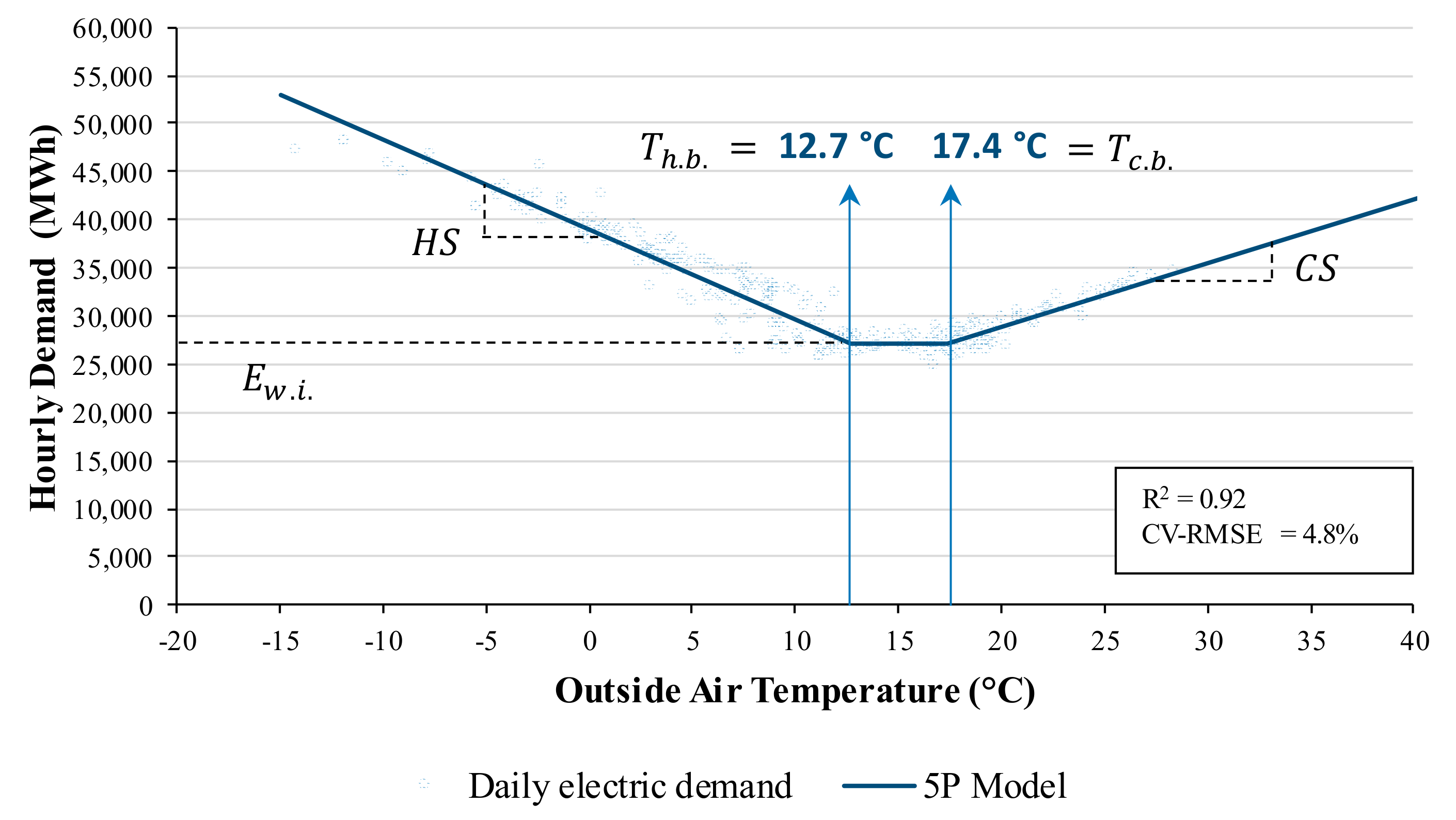
We used the daily electricity demand data from each BA and corresponding daily average OAT data from the NOAA site in a city which is close to the location of a BA on the US EIA map. For most BAs, the 5P change-point model (see Figure 3 and Table 2) was best, indicating substantial energy use for heating in all BAs. Only data from GCPD during the WE period were suitable for the 4P change-point model because it had the same heating and cooling balance-point temperatures. In addition, the data from IID and HST resulted in 3P cooling change-point models because their regions are in the hot climate zones where most buildings do not use energy to heat inside the buildings.
To investigate issues further, the results are presented in graphs ordered lowest to highest for various parameter values in Figure 4, Figure 5, Figure 6 and Figure 7. Figure 4 shows the daily weather-independent energy use for each of the BAs. As one would expect, the magnitude follows with the size of the BA. For example, MISO has the largest number of customers among the 14 BAs. In addition, the types of industry can significantly affect the amount of the weather-independent daily demand. The daily weather-independent demand from the WD period is higher than the WE period from all the BAs. This reason could be that the buildings of the BAs have higher electric internal loads from lighting and equipment during the WD period compared to the WE period. It is interesting to note that the WE demand use is within 10.0% of the WD demand use for all but one of the datasets (the exception being SPA at 11.8%).
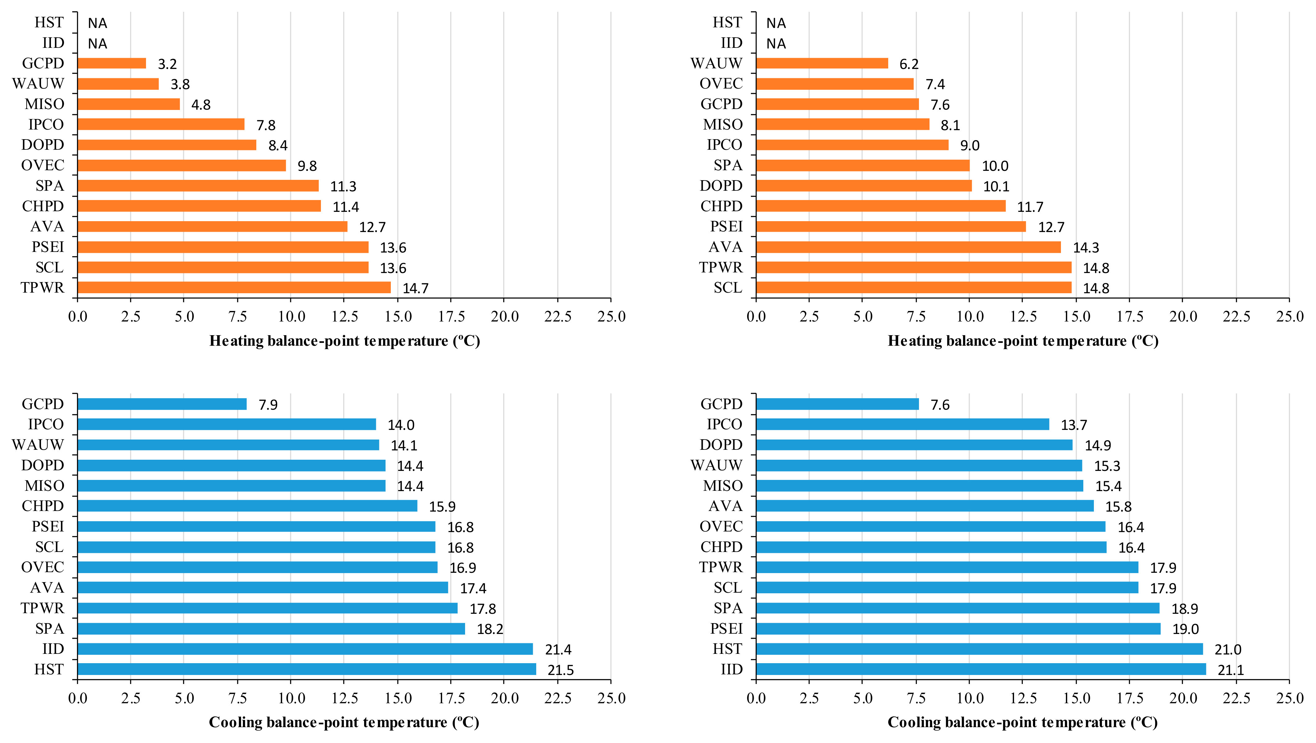
Figure 5 shows the heating and cooling balance-point temperatures (the temperature at which the internal loads balance the environmental loads). The results are interesting in that there is a wide range of values from 3.2 to 14.8 °C for heating and 7.6 to 21.5 °C for cooling balance-point temperatures. One BA in particular seems to stand out. GCPD has an exceptionally low cooling and heating balance-point temperatures. This is likely due to the fact that this region supports an unusually large number of food-processing facilities, many of which produce frozen quantities. In addition, many data-center facilities are located in GCPD. The notably lower set point for these facilities will bring down the average balance temperature considerably.
WAUW shows the second and first lowest heating balance-point temperatures for the WD and WE periods, respectively. This reason could be the coldest climate zone (6B) where the location of WAUW is among the 14 BAs. AVA, PSEI, SCL, and TPWR show relatively high heating balance-point temperatures, even though they are located in the similar climate zones (4C and 5B). The reason could be one of higher heating thermostat setpoints, lower internal loads from lighting or other equipment, and/or higher heat losses through building envelopes of the buildings in the four BAs. HST and IID show the highest cooling balance-point temperatures for both the WD and WE periods. This reason could be the hot climate zones (1A and 2B) where the locations of HST and IID are among the 14 BAs. The higher variance in the heating-balance-point temperatures means that many buildings used different heating setpoints, and heating-balance-point temperatures were more affected by internal loads compared to cooling-balance-point temperatures. It also depends on the types of industry in each BA.
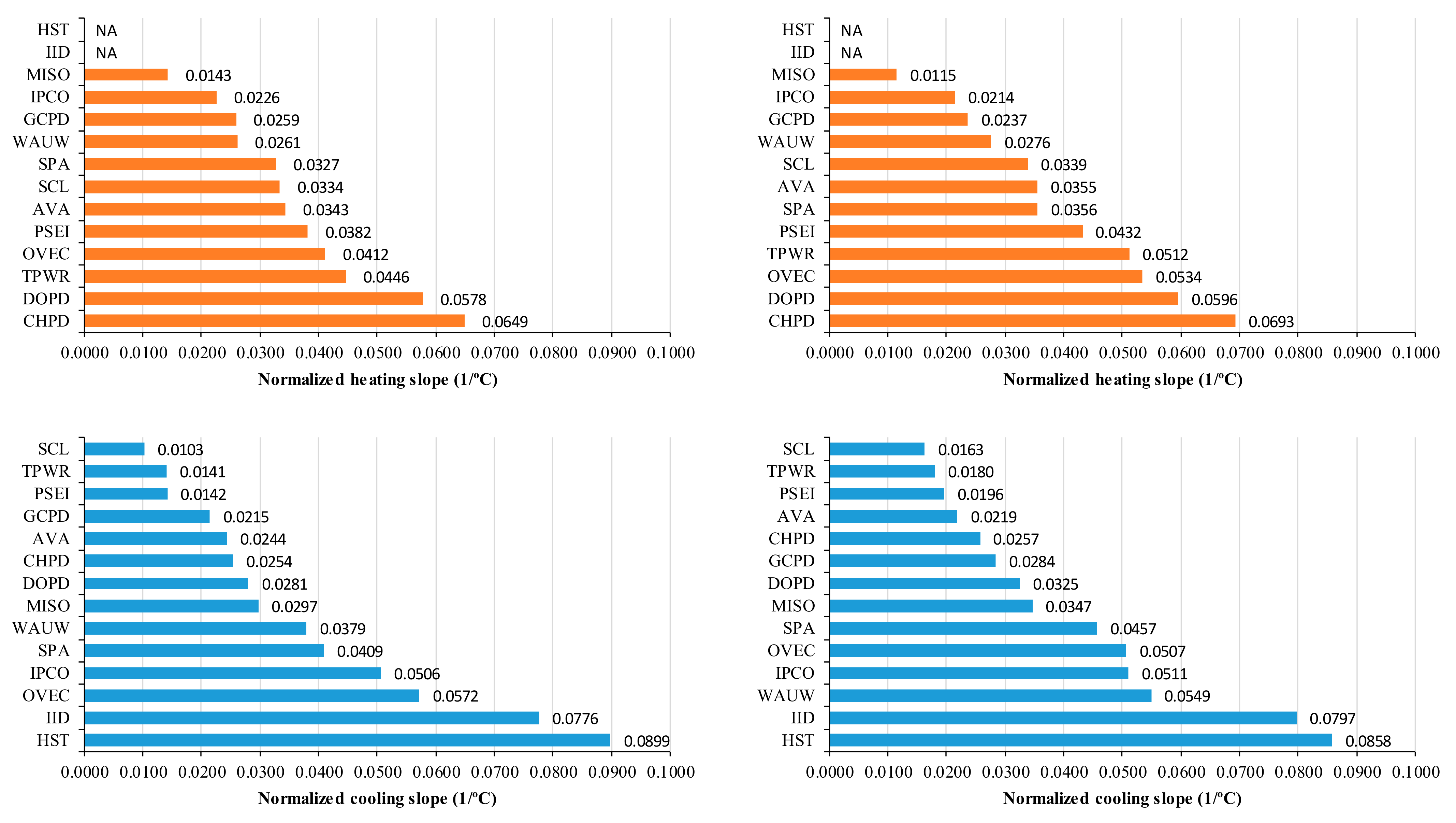
Figure 6 shows the normalized heating and cooling slopes between BAs. MISO, IPCO, GCPD, and WAUW show relatively low normalized heating slopes for both the WD and WE periods. The four BAs show that the normalized heating slopes are 28.1% and 28.9% lower compared to the averages for the WD period and the WE period, respectively. The reason for this could be that the buildings of the BAs have higher efficiency heating systems and/or lower heating loads from weatherization programs. DOPD and CHPD show relatively high normalized heating slopes above 59.0% and 53.4% compared to the averages for the WD and WE periods, respectively. This reason could be that the buildings of the BAs have lower efficiency heating systems (e.g., electric resistance heaters) and/or higher heating loads from lower-quality building envelopes. DOPD and CHPD have the lowest electric rates in the U.S.
SCL, TPWR, and PSEI show relatively low normalized cooling slopes for both the WD and WE periods. The three BAs show that the normalized cooling slopes are 62.0% and 51.4% lower compared to the averages for the WD period and the WE period, respectively. The reason for this could be that the weathers of their cooling periods are very mild, and few buildings in these areas have air conditioning systems. IPCO and OVEC show relatively high normalized cooling slopes that are 35.8% and 25.6% higher compared to the averages for both the WD and WE periods, except HST and IID in the hot climate zones (1A and 2B). The reason for this could be that the buildings of the two BAs have lower efficiency cooling systems and/or higher cooling loads from lower-quality building envelopes. Further comparisons from Figure 4, Figure 5 and Figure 6 are possible if more information was known about the demographics and the characteristics of the loads in the various BAs.
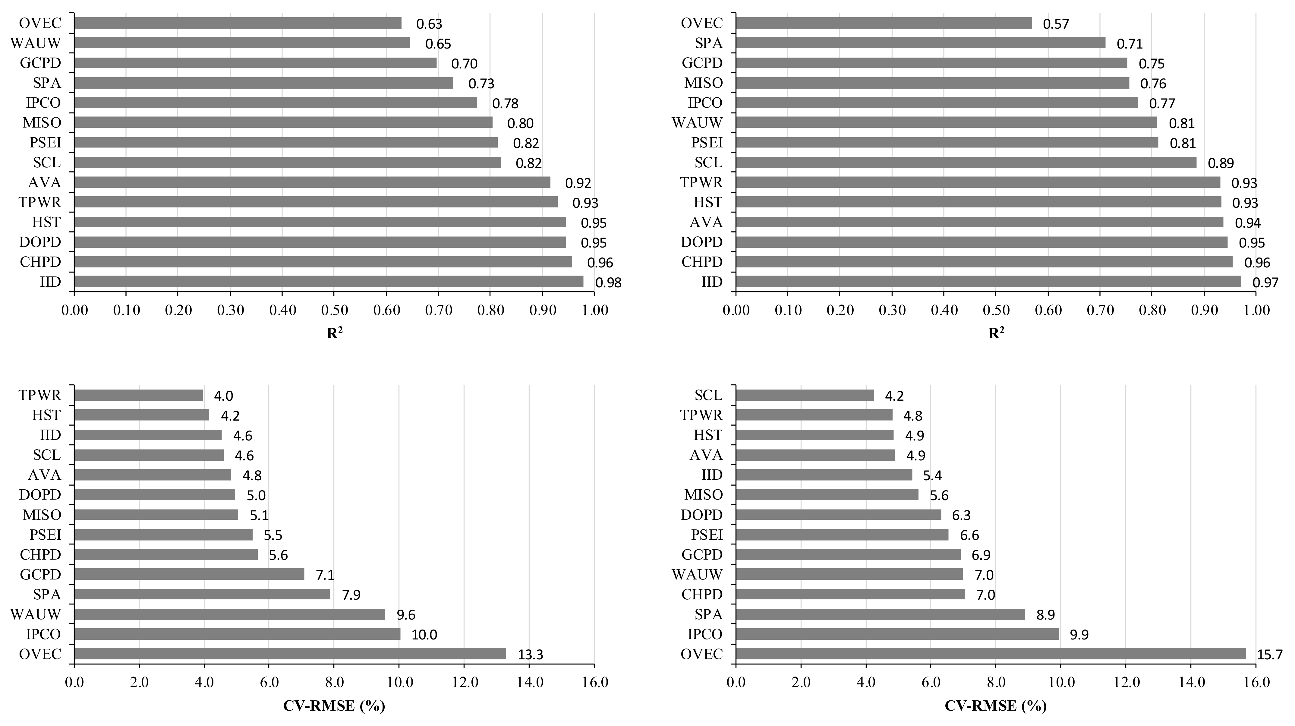
Figure 7 shows the accuracy of the applied change-point linear regression models. OVEC has the most inaccurate model, based on R2 and CV-RMSE. The reason for this could be that the buildings of OVEC have the most variances of building characteristics, system operation schedules, or occupancy schedules among the 14 BAs. The change-point linear regression models of all the BAs, except OVEC, indicate R2 above 0.65 and CV-RMSE below 10.1%, showing that they are well-established models for each BA during the WD and WE periods.

3.2. Results from the Energy Signature Analysis for Four BAs for the Two Different Periods

For further analysis, the four BAs of SCL, IPCO, IID, and HST are selected to compare them with the two different annual periods using the coefficients from the energy signature analysis and a weather-adjusted saving calculation method in order to examine the efficacy of their energy efficiency programs. It is assumed that two different periods are from 1 July 2015 to 30 June 2016 (for a baseline or a pre-energy efficiency program period) and from 1 July 2017 to 30 June 2018 (for a post-energy efficiency program period).
Figure 8 through 11 show the resultant comparisons for the four BAs during the two different periods. In Figure 8, SCL and IPCO have lower weather-independent electricity demand in the 2017–2018 period compared to the 2015–2016 period. The WD and WE use from SCL show the reductions of 3.0% and 3.8%, respectively. The WD and WE use from IPCO also show the reductions of 4.5% and 8.4%, respectively. The reason for this could be that the buildings of the BAs have lower electric internal loads from lighting and equipment due to their energy efficiency programs.
In Figure 9, for the WD period, the heating balance-point temperatures of SCL and IPCO in the 2017–2018 period are higher than those in the 2015–2016 period. For both the WD and WE periods, the cooling balance-point temperatures of IID in the 2017–2018 period are higher than those in the 2015–2016 period. However, the cooling balance-point temperatures of SCL and IPCO in the 2017–2018 period are lower than the 2015–2016 period. The trends from the balance-point temperature analysis do not show a strong effect from the energy efficiency program of weatherization because the weatherization program normally causes a lower heating-balance-point temperature and a higher cooling balance-point temperature.
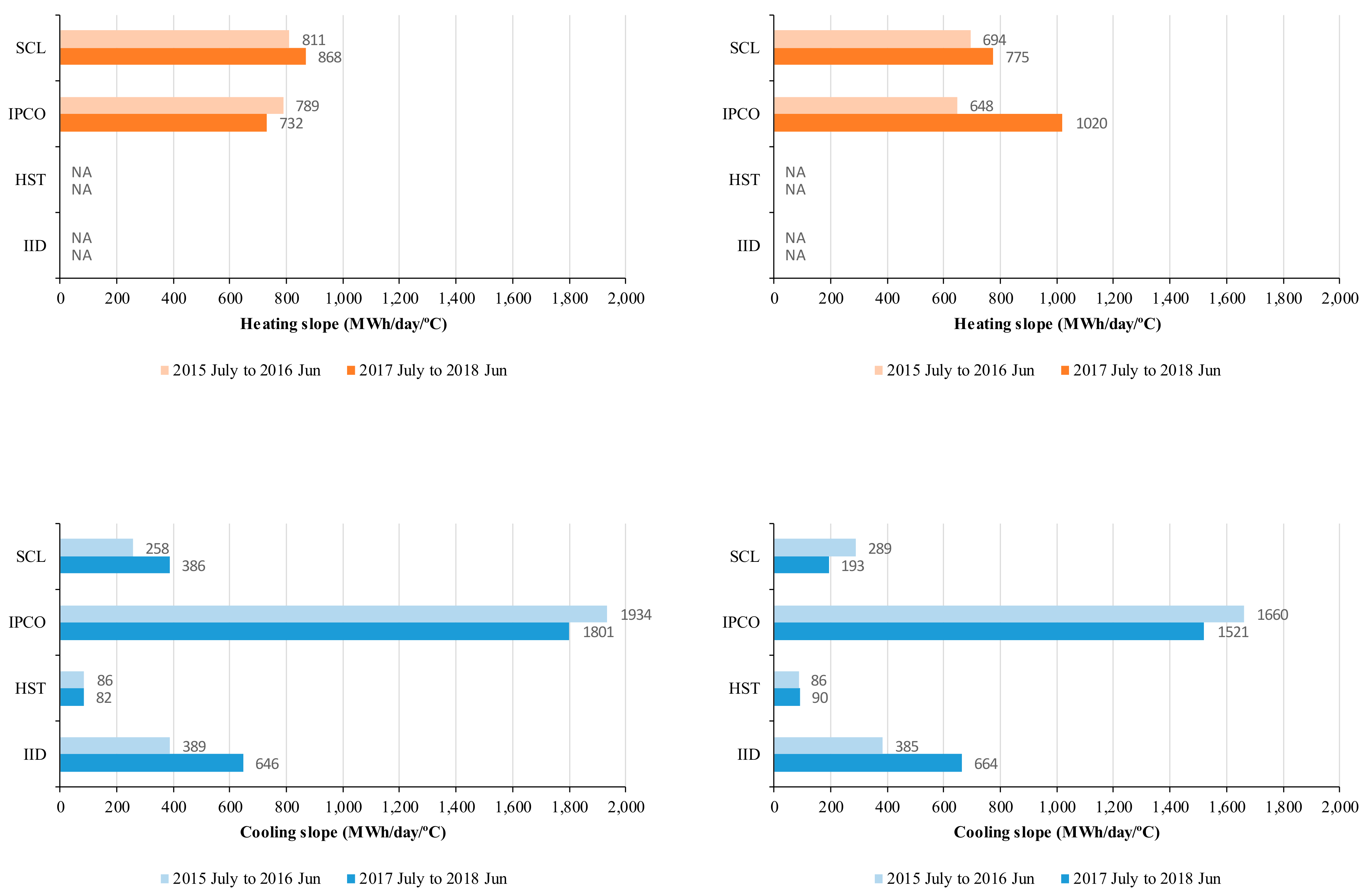
In Figure 10, SCL shows that both the WD and WE heating slopes in the 2017–2018 period are higher than the 2015–2016 period. This reason could be that the buildings in SCL have more aggressive system-on schedules in the 2017–2018 period. IPCO shows a much higher heating slope for the WEs in the 2017–2018 period, but a lower heating slope for the WDs. The reason for this could be that the buildings in IPCO have the abnormal system-on schedules for the WEs in the 2017–2018 period. A further survey would be needed to explore this particular trend. In terms of the cooling slopes, IPCO have lower cooling slopes for both the WDs and WEs in the 2017–2018 period, which could mean that the buildings in IPCO have higher efficiency cooling systems or system schedules from IPCO’s energy efficiency program and/or less cooling loads from its weatherization program.
Based on the signature analysis from the coefficient comparisons, SCL and IPCO have a high likelihood that they could effectively implement their energy efficiency programs for the buildings because they show significant reductions from the weather-independent electricity demand in the 2017–2018 period. Furthermore, IPCO’s lower cooling slopes in the 2017–2018 period could prove the implementation of its energy efficient program for the cooling systems and/or cooling loads in the buildings.
To quantify and estimate energy savings from the four BAs’ energy efficiency programs, a weather-adjusted saving calculation method was used. The resultant electricity demand is shown in Table 3. As it was estimated in the energy signature analysis, SCL and IPCO have lower electricity demand in the 2017–2018 period compared to the baseline 2015–2016 period. The annual electricity demand reductions for SCL and IPCO are 136,655 MWh (1.5%) and 182,053 MWh (1.1%), respectively. However, it is observed that HST and IID might not have their energy efficiency programs or the energy efficiency programs were not effectively implemented yet because their annual electricity demand in the 2017–2018 period are increased.
Based on the IPCO’s annual reports, the estimated energy savings is 187,474 MWh in the 2017–2018 period [36,37]. The assumption on the estimated savings was the average of the estimated savings in the 2017 and 2018 annual reports because the period used for this analysis was from July 2017 to June 2018. The estimated savings from the weather-adjusted method is 182,053 MWh, so the difference is only −5371 MWh (−2.87%). A time-series analysis was also conducted for IPCO. Figure 11 shows measured daily electricity demand during the 2017 to 2018 period compared to the adjusted baseline daily electricity demand, as well as corresponding outside air temperature data. The significant demand reductions occurred from the middle of September to the end of November and from the middle of March to the middle of April when outside air temperatures are between the heating balance-point temperature of 7.5 °C and the cooling balance-point temperature of 15.0 °C (i.e., a weather-independent period inside the green lines in the figure). The heating and cooling balance-point temperatures were calculated using the weighted average during the baseline’s WD and WE periods. However, for the heating and cooling periods when outside air temperatures are below the heating balance-point temperature and above the cooling balance-point temperature, respectively, the demand shows decreases or increases in fluctuations. In addition, using the CO2 emission factors for Idaho in 2017 and 2018 [38,39], the carbon footprint was calculated. It was estimated that the highest CO2 emission of 11,865 ton was occurred on 14 June 2018, and the lowest carbon footprint of −9521 ton was occurred on 29 October 2017.

4. Discussion

This paper suggests the analysis approach for the publicly available aggregate electricity loads from entire Balancing Authorities (BAs). The same approach used for building energy signature was applied to these datasets, and although the approach uses the assumption of a uniform environmental temperature for all electric loads, which is clearly violated in the case of BAs, the analysis results in surprisingly coherent regressions using the daily intervals. Of the 14 BAs analyzed, only the two BAs (WAUW in central Montana and OVEC in Southern Ohio) resulted in R2 values below 0.70, and the six BAs (TPWR, AVA, CHPD, DOPD, IID, and HST) resulted in R2 values above 0.90 for both the WD and WE datasets. Perhaps the most convincing result for the robustness of this method is that the model for MISO, which covers a wide range of weather patterns from the continent in the north through the Great Lakes and into the Great Plains, had the R2 value of 0.80 on the weekdays with CV-RMSE of 5.1% and R2 of 0.76 on the weekends/holidays with CV-RMSE of 5.6%. However, to identify the reasons of low R2, a future study should analyze the energy patterns of the BAs with a knowledge-based database including the surveys of demographics, industry types, etc.
Additionally, the addition of normalized heating and cooling slopes was proposed. By normalizing the temperature-dependent coefficients with the weather-independent annual energy consumption, it opens the opportunity to make a consistent comparison of temperature dependence between BAs. Although this particular index of performance will require further refinement, these results show promise. For example, the analysis shows that BAs in hot climates (IID and HST) have the largest normalized cooling slopes, while the two worst for heating (CHPD and DOPD) are located in central Washington. This may be due to the fact that these two BAs have the lowest electricity rates in the U.S., so many buildings have electric resistance heaters that are not energy efficient.
We examined a possible application of this approach by developing a model for a one-year dataset, then using that model to estimate whether energy use in a subsequent year was higher or lower taking different weather into account. By using the baseline model, we estimate how much energy would have been consumed in the subsequent year if nothing, except the changes from their energy efficiency programs, had changed in the BA. By comparing that number to the actual energy consumption, we analyzed weather-normalized measures of how the load in a particular area is evolving. This can have significant impacts for both utility planners and those responsible for verifying the efficacy of their energy efficiency programs. Our analysis shows that the estimated decrease in electricity consumption in IPCO is very close to the amount of savings reported from their energy efficiency programs in the intervening year. This analysis requires the assumption that there was no significant change in overall loads between the two periods, an assumption that might not always be reasonable, but is generally accepted for the period under analysis. For better analysis, we may need to obtain the detailed information on demographic/firmographic locations and changes, economic conditions, natural conservation, building codes and standards, building types, etc., however, the approaches suggested in this paper can be useful for utility managers to effectively verify the energy efficiency programs in their regions.

5. Conclusions

We conducted an energy signature analysis for BAs using publicly available data. We also suggested an analysis method that allows for meaningful comparisons between BAs and to assess changes in time for a given BA which could be used to interpret changes in load patterns year-to-year, accounting for changes in weather. As an example, this approach can be used to verify the impact of energy efficiency programs on a building component/system-wide basis.
The application of building energy signature analysis to entire BAs results in surprisingly coherent models of the relationship between daily electricity consumption and corresponding daily average outside temperature. The resulting model that categorizes weather-dependent and weather-independent electric loads in the large areas can be used for a number of purposes, including tracking the characteristics of the load for a given BA from year to year, predicting future load growth due to a warming climate, estimating the efficacy of energy efficiency programs, and validating other load models used by utility planners. The normalization of these models shows some promise, but requires further refinement and validation before it can be truly useful.
Ultimately, the analysis approach in this paper was conducted in order to examine the effectiveness of an energy efficiency program’s implementation. Energy efficiency stakeholders can use this approach to survey how well energy efficiency programs are implemented in their regions. If it is provided that how many buildings and types of buildings are serviced by each BA, this approach will be more interpretable with less uncertainty. Even though it has limitations, this analysis approach shows promising benefits from the use of the publicly available BA-level aggregate electric loads. This approach can be used as a tool to better understand the electric loads from BAs. For future work, the uncertainty of the analysis approach will be checked with knowledge-based data from BAs.

Author Contributions

Conceptualization, S.O. and J.F.G.; methodology, S.O. and J.F.G.; software, S.O.; validation, S.O.; formal analysis, S.O.; investigation, S.O.; resources, S.O.; data curation, S.O.; writing—original draft preparation, S.O.; writing—review and editing, J.F.G.; visualization, S.O.; supervision, S.O. and J.F.G. All authors have read and agreed to the published version of the manuscript.

Funding

This research was supported by the Major Project of the Korea Institute of Civil Engineering and Building Technology (KICT) (grant number 20220156-001).

Institutional Review Board Statement

Not applicable.

Informed Consent Statement

Not applicable.

Data Availability Statement

Not applicable.

Acknowledgments

The authors would like to thank Kathleen Araújo, a director of the Energy Policy Institute at Boise State University, and Damon Woods, an interim director at the Integrated Design Lab at University of Idaho, for their valuable comments for this paper.

Conflicts of Interest

The authors declare no conflict of interest.

References

  1. ACEEE. State and Utility Policy. Available online: https://www.aceee.org/program/utilities (accessed on 27 June 2022).
  2. Austin Energy Rebates & Incentives. Available online: https://savings.austinenergy.com/rebates/ (accessed on 27 June 2022).
  3. Idaho Power Ways to Save. Available online: https://www.idahopower.com/energy-environment/ways-to-save/ (accessed on 27 June 2022).
  4. Berg, W.; Ribeiro, D. Saving Watts to Save Drops: Inclusion of Water Efficiency in Energy Efficiency Programs; American Council for an Energy-Efficient Economy: Washington, DC, USA, 2018. [Google Scholar]
  5. Bukarica, V.; Tomšić, Ž. Energy Efficiency Policy Evaluation by Moving from Techno-Economic towards Whole Society Perspective on Energy Efficiency Market. Renew. Sustain. Energy Rev. 2017, 70, 968–975. [Google Scholar] [CrossRef]
  6. ACEEE. State and Local Policy Database. Available online: https://database.aceee.org/ (accessed on 27 June 2022).
  7. Hayes, S.; Baum, N.; Herndon, G. Energy Efficiency: Is the United States Improving? American Council for an Energy-Efficient Economy: Washington, DC, USA, 2013. [Google Scholar]
  8. Perez, K.X.; Cetin, K.; Baldea, M.; Edgar, T.F. Development and Analysis of Residential Change-Point Models from Smart Meter Data. Energy Build. 2017, 139, 351–359. [Google Scholar] [CrossRef] [Green Version]
  9. Kissock, J.K.; Reddy, T.A.; Claridge, D.E. Ambient-Temperature Regression Analysis for Estimating Retrofit Savings in Commercial Buildings. ASME J. Sol. Energy Eng. 1998, 120, 168–176. [Google Scholar] [CrossRef]
  10. Kissock, K.J.; Eger, C. Measuring Industrial Energy Savings. Appl. Energy 2008, 85, 347–361. [Google Scholar] [CrossRef]
  11. ASHRAE. Chapter 19. Energy Estimating and Modeling Methods. In ASHRAE Handbook—Fundamentals; ASHRAE: Atlanta, GA, USA, 2017. [Google Scholar]
  12. Fumo, N.; Rafe Biswas, M.A. Regression Analysis for Prediction of Residential Energy Consumption. Renew. Sustain. Energy Rev. 2015, 47, 332–343. [Google Scholar] [CrossRef]
  13. Raffio, G.; Isambert, O.; Mertz, G.; Schreier, C.; Kissock, K. Targeting Residential Energy Assistance. In Proceedings of the ASME 2007 Energy Sustainability Conference, Long Beach, CA, USA, 27–30 July 2007; pp. 489–495. [Google Scholar]
  14. Gianniou, P.; Reinhart, C.; Hsu, D.; Heller, A.; Rode, C. Estimation of Temperature Setpoints and Heat Transfer Coefficients among Residential Buildings in Denmark Based on Smart Meter Data. Build. Environ. 2018, 139, 125–133. [Google Scholar] [CrossRef]
  15. Eriksson, M.; Akander, J.; Moshfegh, B. Investigating Energy Use in a City District in Nordic Climate Using Energy Signature. Energies 2022, 15, 1907. [Google Scholar] [CrossRef]
  16. Ding, Y.; Ivanko, D.; Cao, G.; Brattebø, H.; Nord, N. Analysis of Electricity Use and Economic Impacts for Buildings with Electric Heating under Lockdown Conditions: Examples for Educational Buildings and Residential Buildings in Norway. Sustain. Cities Soc. 2021, 74, 103253. [Google Scholar] [CrossRef]
  17. Aragon, V.; James, P.A.B.; Gauthier, S. The Influence of Weather on Heat Demand Profiles in UK Social Housing Tower Blocks. Build. Environ. 2022, 219, 109101. [Google Scholar] [CrossRef]
  18. Ali, M.T.; Mokhtar, M.; Chiesa, M.; Armstrong, P. A Cooling Change-Point Model of Community-Aggregate Electrical Load. Energy Build. 2011, 43, 28–37. [Google Scholar] [CrossRef]
  19. Wang, Z.; Hong, T.; Li, H.; Ann Piette, M. Predicting City-Scale Daily Electricity Consumption Using Data-Driven Models. Adv. Appl. Energy 2021, 2, 100025. [Google Scholar] [CrossRef]
  20. US EIA. U.S. Electric System Operating Data. Available online: https://www.eia.gov/realtime_grid/#/status?end=20180830T17 (accessed on 30 August 2018).
  21. US EIA. About the EIA-930 Data. Available online: https://www.eia.gov/electricity/gridmonitor/about (accessed on 27 June 2022).
  22. US EIA. Hourly Electric Grid Monitor. Available online: https://www.eia.gov/electricity/gridmonitor/dashboard/electric_overview/US48/US48 (accessed on 29 April 2022).
  23. Ruggles, T.H.; Farnham, D.J.; Tong, D.; Caldeira, K. Developing Reliable Hourly Electricity Demand Data through Screening and Imputation. Sci. Data 2020, 7, 155. [Google Scholar] [CrossRef] [PubMed]
  24. Büyükalaca, O.; Bulut, H.; Yılmaz, T. Analysis of Variable-Base Heating and Cooling Degree-Days for Turkey. Appl. Energy 2001, 69, 269–283. [Google Scholar] [CrossRef] [Green Version]
  25. US EIA. Hourly Information on U.S. Electricity Supply, Demand, and Flows Is Now Available. Available online: https://www.eia.gov/todayinenergy/detail.php?id=27212 (accessed on 27 August 2018).
  26. US EIA. EIA-930 Data Users Guide and Known Issues; US EIA: Washington, DC, USA, 2018. [Google Scholar]
  27. US EIA. U.S. Electric Power Regions. Available online: https://www.eia.gov/todayinenergy/detail.php?id=27152 (accessed on 6 August 2018).
  28. US EIA. Select Balancing Authority. Available online: https://www.eia.gov/electricity/gridmonitor/dashboard/electric_overview/US48/US48 (accessed on 27 June 2022).
  29. ICC. 2018 International Energy Conservation Code; ICC: Washington, DC, USA, 2017. [Google Scholar]
  30. NOAA. Data Tools: Local Climatological Data (LCD). Available online: https://www.ncdc.noaa.gov/cdo-web/datatools/lcd (accessed on 1 July 2018).
  31. Long, N. Real-Time Weather Data Access Guide; National Renewable Energy Laboratory: Golden, CO, USA, 2006. [Google Scholar]
  32. Kissock, K.; Haberl, J.S.; Claridge, D.E. Inverse Modeling Toolkit: User’s Guide (ASHRAE Final Report for RP-1050); ASHRAE: Atlanta, GA, USA, 2001. [Google Scholar]
  33. ASHRAE. ASHRAE Guideline 14-2014; ASHRAE: Atlanta, GA, USA, 2014. [Google Scholar]
  34. Research Into Action; QuEST; Stetz Consulting; Kolderup Consulting; Warren Energy Engineering; Left Fork Energy; Consulting, S. Regression for M & V: Reference Guide; Bonneville Power Administration (BPA): Portland, OR, USA, 2011. [Google Scholar]
  35. Henseler, J.; Ringle, C.M.; Sinkovics, R.R. The Use of Partial Least Squares Path Modeling in International Marketing. In New Challenges to International Marketing; Sinkovics, R.R., Ghauri, P.N., Eds.; Advances in International Marketing; Emerald Group Publishing Limited: Bingley, UK, 2009; Volume 20, pp. 277–319. ISBN 978-1-84855-468-9. [Google Scholar]
  36. Idaho Power. Demand-Side Management 2017 Annual Report; Idaho Power: Boise, ID, USA, 2018. [Google Scholar]
  37. Idaho Power. Demand-Side Management 2018 Annual Report; Idaho Power: Boise, ID, USA, 2019. [Google Scholar]
  38. US EIA. Idaho Electricity Profile 2017—Table 1. Available online: https://www.eia.gov/electricity/state/archive/2017/idaho/ (accessed on 28 June 2022).
  39. US EIA. Idaho Electricity Profile 2018—Table 1. Available online: https://www.eia.gov/electricity/state/archive/2018/idaho/ (accessed on 28 June 2022).
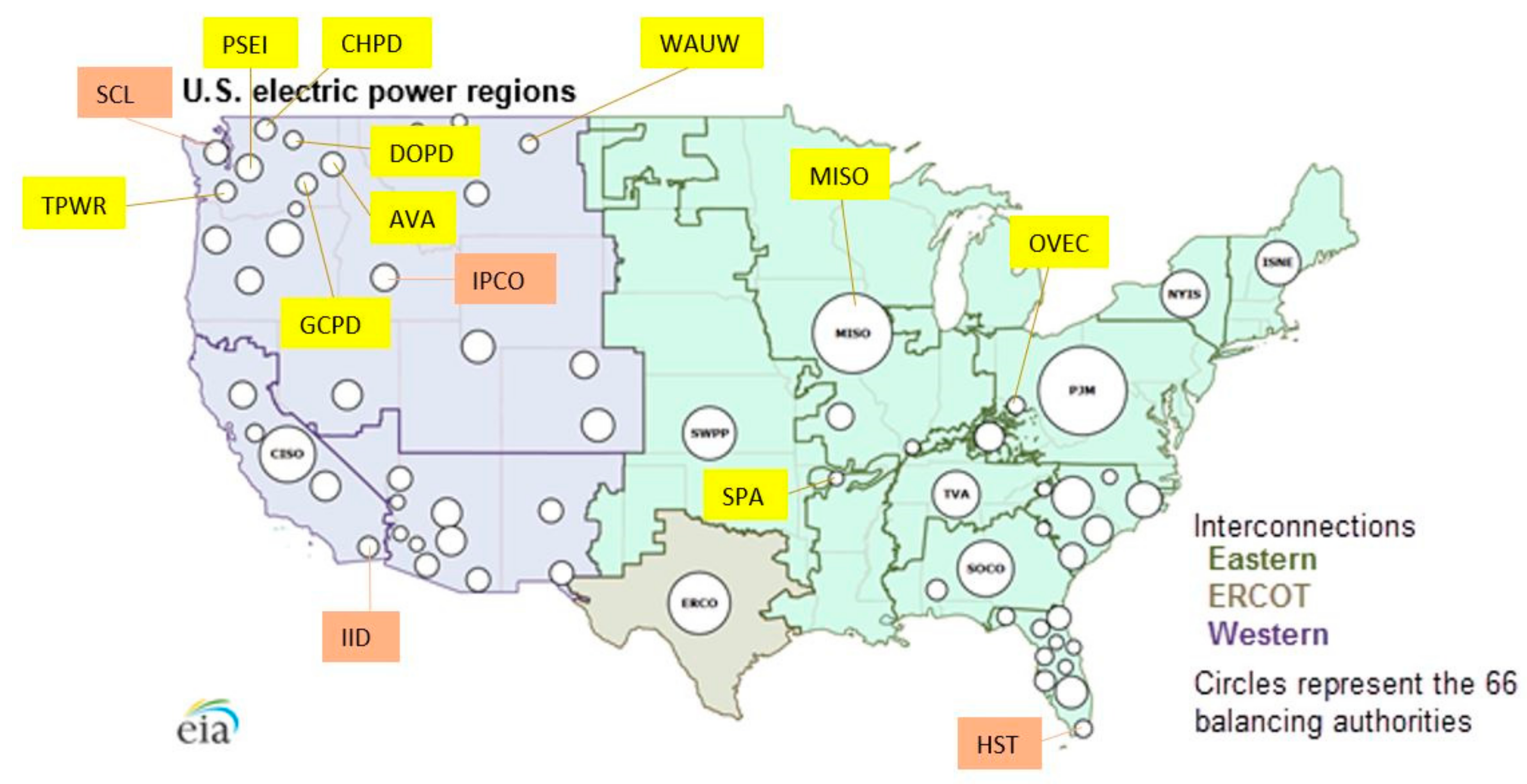
Figure 1. Balancing Authorities (BAs) and selected BAs in U.S. electric power regions. Adapted from [27,28].
Sustainability 14 08649 g001
Figure 2. Overall methodology.
Sustainability 14 08649 g002
Figure 3. The 5P model for AVA using the daily electricity demand and corresponding OAT data during the WD period in 2016.
Sustainability 14 08649 g003
Figure 4. Comparison of weather-independent daily demand for the weekdays (left) and the weekends/holidays (right) in 2016.
Sustainability 14 08649 g004
Figure 5. Comparison of balance-point temperatures for the weekdays (left) and the weekends/holidays (right) in 2016.
Sustainability 14 08649 g005
Figure 6. Comparison of normalized heating slopes (absolute values) and cooling slopes for the weekdays (left) and the weekends/holidays (right) in 2016.
Sustainability 14 08649 g006
Figure 7. Comparison of R2 and CV-RMSE (%) for the weekdays (left) and the weekends/holidays (right) in 2016.
Sustainability 14 08649 g007
Figure 8. Comparison of weather-independent daily demand for the weekdays (left) and the weekends/holidays (right) in the two different periods.
Sustainability 14 08649 g008
Figure 9. Comparison of heating and cooling balance-point temperatures for the weekdays (left) and the weekends/holidays (right) in the two different periods.
Sustainability 14 08649 g009
Figure 10. Comparison of heating slopes (absolute values) and cooling slopes for the weekdays (left) and the weekends/holidays (right) in the two different periods.
Sustainability 14 08649 g010
Figure 11. Time series for IPCO’s measured daily electricity demand during the post-energy efficient program period with the adjusted baseline daily electricity demand as well as the corresponding outside air temperature (For better visualization, missing data were filled in using a linear interpolation).
Sustainability 14 08649 g011
Table 1. List of selected BAs.
BARegionIECC Climate ZoneWeather Data (NOAA)
Location, State
Seattle City Light (SCL)Northwest4CSeattle-Tacoma, WA
City of Tacoma, Department of Public Utilities, Light Division (TPWR)Northwest4CSeattle-Tacoma, WA
Puget Sound Energy, Inc. (PSEI)Northwest5BSeattle-Tacoma, WA
Public Utility District No. 2 of Grant County, Washington (GCPD)Northwest5BSpokane, WA
Avista Corporation (AVA)Northwest5BSpokane, WA
Public Utility District No. 1 of Chelan County (CHPD)Northwest5BOmak, WA
PUD No. 1 of Douglas County (DOPD)Northwest5BOmak, WA
Idaho Power Company (IPCO)Northwest5BBoise, ID
Western Area Power Administration—Upper Great Plains West (WAUW)Northwest6BGlasgow, MT
Imperial Irrigation District (IID)California2BEL Centro, CA
Southwestern Power Administration (SPA)Central4AHarrison, AR
Ohio Valley Electric Corporation (OVEC)Mid-Atlantic4ACincinnati, OH
City of Homestead (HST)Florida1AMiami, FL
Midcontinent Independent System Operator, Inc. (MISO)Midwest5ADes Moines, IA
Table 2. Summary of the change-point linear regression model results from daily BA electricity demand data for the 2016 period.
BAWeather Data (NOAA), StateWD/WEMissing/
Outlier Days
Used model T h . b .   ( ° C ) T c . b .   ( ° C ) H S   ( MWh / day / °C) C S   ( MWh / day / °C) Normalized   H S   ( 1 / ° C ) Normalized   C S   ( 1 / ° C ) E w . i .   ( MWh / Day ) R2CV-RMSE (%)
SCLSeattle-Tacoma,WD4/05P13.616.8−817.6251.7−0.03340.010324,469.70.824.6%
WAWE2/05P14.817.9−758.3364.6−0.03390.016322,398.00.894.2%
TPWRSeattle-Tacoma,WD0/05P14.717.8−516.9162.8−0.04460.014111,580.60.934.0%
WAWE0/05P14.817.9−535.5188.0−0.05120.018010,459.50.934.8%
PSEISeattle-Tacoma,WD3>/05P13.616.8−2,822.11,047.5−0.03820.014273,919.60.825.5%
WAWE2/05P12.719.0−3,026.71,375.6−0.04320.019670,104.20.816.6%
GCPDSpokane,WD0/05P3.27.9−298.7247.7−0.02590.021511,531.30.707.1%
WAWE0/04P7.67.6−247.4297.0−0.02370.028410,448.00.756.9%
AVASpokane,WD0/25P12.717.4−933.1661.7−0.03430.024427,173.40.924.8%
WAWE0/25P14.315.8−871.3537.2−0.03550.021924,531.30.944.9%
CHPDOmak,WD0/05P11.415.9−230.690.3−0.06490.02543554.20.965.6%
WAWE0/05P11.716.4−233.286.5−0.06930.02573366.60.967.0%
DOPDOmak,WD11/05P8.414.4−185.089.8−0.05780.02813201.20.955.0%
WAWE4/05P10.114.9−174.194.9−0.05960.03252922.80.956.3%
IPCOBoise,WD1/75P7.814.0−873.11,960.0−0.02260.050638,710.90.7810.0%
IDWE2/35P9.013.7−780.91,861.6−0.02140.051136,459.90.779.9%
WAUWGlasgowWD28/15P3.814.1−48.570.4−0.02610.03791,855.20.659.6%
MTWE30/05P6.215.3−48.295.8−0.02760.05491744.70.817.0%
IIDEL Centro,WD5/03P21.421.40.0582.60.00000.07767506.40.984.6%
CAWE5/03P21.121.10.0546.70.00000.07976856.40.975.4%
SPAHarrison,WD0/05P11.318.2−50.863.6−0.03270.04091553.80.737.9%
ARWE0/05P10.018.9−48.862.6−0.03560.04571370.10.718.9%
OVECCincinnati,WD0/15P9.816.9−65.691.1−0.04120.05721592.70.6313.3%
OHWE1/05P7.416.4−79.074.9−0.05340.05071477.50.5715.7%
HSTMiami,WD3/03P21.521.50.097.40.00000.08991084.30.954.2%
FLWE0/03P21.021.00.091.40.00000.08581064.90.934.9%
MISODes MoinesWD2/05P4.814.4−23,450.948,687.5−0.01430.02971,638,332.90.805.1%
IAWE1/05P8.115.4−17,020.551,193.9−0.01150.03471,476,414.60.765.6%
Table 3. Four BAs’ measured electricity demand compared to the adjusted (predicted) baseline electricity demand in the 2017 to 2018 period, as well as measured electricity demand in the 2015 to 2016 period.
BAPeriodWD/WEMeasured
(MWh)
Adjusted
Baseline
(MWh)
Difference
(MWh)
Difference
(%)
SCLJuly 2015–June 2016WD6,806,550
WE2,874,378
Total9,680,928
July 2017–June 2018WD6,413,6116,502,737−89,126−1.4%
WE2,672,6952,720,224−47,529−1.7%
Total9,086,3069,222,961−136,655−1.5%
IPCOJuly 2015–June 2016WD11,899,065
WE4,974,351
Total16,873,416
July 2017–June 2018WD10,934,42511,050,100−115,675−1.0%
WE4,751,9404,818,318−66,378−1.4%
Total15,686,36515,868,418−182,053−1.1%
HSTJuly 2015–June 2016WD328,037
WE150,258
Total478,295
July 2017–June 2018WD352,822350,63621860.6%
WE156,657157,539−882−0.6%
Total509,479508,17613030.3%
IIDJuly 2015–June 2016WD2,331,221
WE923,900
Total3,255,121
July 2017–June 2018WD2,338,6332,132,910205,7239.6%
WE972,205863,453108,75212.6%
Total3,310,8382,996,362314,47610.5%
Publisher’s Note: MDPI stays neutral with regard to jurisdictional claims in published maps and institutional affiliations.