Abstract
With the increase in people’s travel demands, the air pollution generated by the means of transportation they take is also becoming more and more serious. Among them, in the process of people’s travel, the exhaust pollution caused by traffic congestion is particularly serious. Accurately identifying various regimes of oversaturation and taking effective control strategies play a key role in alleviating traffic congestion. There are three regimes of evolution during an oversaturated scenario: loading, oversaturated operation, and recovery. In the traffic signal control under the oversaturated scenario, the corresponding control targets and methods should be adopted based on the regime of oversaturation. In this paper, the multi-objective attributes and their trajectory data of each movement at the intersection are analyzed. Based on the oversaturation severity index, the traffic volume, and the queuing on the movement, the identification and cause analysis of each regime of the oversaturation are carried out. The examples and simulation results proved that the method proposed in this paper could effectively analyze the cause and degree of oversaturation and identify its regime. This has important implications for alleviating traffic congestion and reducing vehicle carbon emissions.
1. Introduction
Traffic congestion is an ongoing problem that leads to noise, air pollution, and energy consumption [1,2,3], and intersection oversaturation is one of the main manifestations of traffic congestion. In the loading, oversaturated operation, and recovery regimes of intersection oversaturation, it is of great significance to accurately identify its regime and cause and combine relevant theories to manage the traffic, which is of great significance for improving levels of service and alleviating or even avoiding oversaturated traffic conditions. Moreover, the traffic flow at an intersection is composed of traffic flows in different movements. When analyzing the oversaturation regimes, the research goal is focused on each movement, which can more accurately analyze the regimes and cause of the intersection, adopt appropriate traffic control strategies, alleviate urban traffic congestion or accidents [4,5], and finally, improve air quality [6,7].
Traffic control under supersaturated conditions is one of the hot issues studied by experts and scholars in the field of traffic. Noaeen et al. [8] proposed a traffic signal control method by lane-based queue measurements, aiming at maximizing the individual effective outflow rate of each movement and alleviating the negative impact of overflow in the network. Sun et al. [9] proposed a queue-based quasi-optimal feedback control strategy, which controls the maximum queue length during the queuing period and clears the queuing queue as soon as possible during the dissipation period. Ding et al. [10] proposed a traffic guidance–perimeter control coupled method, aiming at the optimal cumulative flow and minimum delay of the network and improving the performance of the macro network according to the balance rules of traffic flow in multiple MFD sub-regions. Mariotte et al. [11] proposed a congestion propagation model based on the accumulation model and analyzed the traffic congestion categories by different travel distances or categories, then put forward a control method based on travel demand to achieve control of traffic congestion. Mehdi et al. [12] proposed a traffic flow allocation method based on queue length or delay, which reduces delays while reducing traffic disturbance upstream and preventing oversaturation from spreading further. Mo et al. [13] designed a set of macroscopic fundamental diagram (MFD) partition methods based on graph theory, which is based on the analysis of MFD partition purposes and can be applied to traffic control to prevent traffic congestion transfer, as well as improve road network efficiency. These methods aim to optimize some observable indicators such as queue length, delay, or traffic volume to implement traffic control at oversaturation intersections. Although they have achieved certain results, the quantitative analysis of oversaturated traffic states is insufficient. The situation suggests that demand management policies require consideration of more detailed conditions to improve usability [14].
Wu et al. [15] studied the moving process of traffic flow on the approach of signalized intersections, then proposed a method of traffic status identification based on queue length and approach capacity. Lian et al. [16] used the evaluation method of fuzzy comprehensive analysis to comprehensively analyze the travel speed, saturation, delay, and other indicators of the traffic flow on the main road, to evaluate the traffic condition of the main road in the city. Wang et al. [17] aimed at the problem that the traffic state discrimination method at the intersection could not effectively identify the overflow and slow vehicles, put forward a method to discriminate the traffic status of the intersection in each direction by calculating the saturation. Chen et al. [18] proposed a traffic state combined with signal control and its authenticity discrimination method, using the variance of the headway and time occupancy as the discriminant parameters, combined with the dissipation of queued vehicles in the cycle to discriminate the traffic state. Based on the game theory-cloud model, Xu et al. [19] selected the average speed, saturation, average number of stops, and travel time of the intersection as the basic evaluation indicators and realized the evaluation and analysis of the micro–meso–macro traffic operation state layer by layer. Zhang et al. [20] started from the relationship between the flow of each stage and the split at the intersection, then used the method of comprehensive projection to give a method for defining the traffic state of a multi-stage-controlled intersection. Yao et al. [21] proposed a method to estimate the spillover queue length in the case of low-resolution detection data, cross-analyze the detection data of the upstream and downstream intersections, then use the traffic shockwave theory to describe it. The queue length under the offset conditions is used to calculate the queue length and evaluate it. Chen et al. [22] proposed a spatial queue model for oversaturated traffic system with a time-dependent vehicle arrival rate, then described the evolution process of congestion at the traffic bottleneck by using the flow, density, and travel time at the traffic bottleneck. Yuan et al. [23] proposed a method for identifying traffic bottlenecks and quantifying the degree of traffic congestion by establishing a discrete-time model for traffic bottlenecks to analyze signal timing and traffic flow characteristics. Aljamal et al. [24] proposed a nonlinear filtering approach to estimate the traffic stream density on signalized approaches based solely on connected vehicle data and then evaluate the degree of traffic congestion. Although these methods provide a reference for the quantification of the degree of oversaturation, the obtained oversaturation severity index is difficult to combine with the traffic signal control parameters, and it is difficult to directly control the traffic signal according to the obtained quantification degree.
Some experts and scholars combined the parameters of traffic signal control and put forward the analysis basis for the oversaturated state. Gazis [25] pointed out that the condition of queuing vehicles not completely dissipated within a green light cycle is an oversaturated state. Abu-Lebdeh and Benekohal [26,27] proposed that the multiple queues of vehicles due to insufficient green time or due to congestion can be used as the identification basis for oversaturation conditions. Roess [28] pointed out that the oversaturated state can be discriminated by the unstable queuing characteristics caused by congestion. This view holds that, even when the maximum queue length is less than the length of the road segment, an intersection should be oversaturated if there is a residual queue at the intersection every cycle.
NCHRP (National Cooperative Highway Research Program) [29] defined traffic flow saturation in its report and proposed a temporal oversaturation severity index (TOSI) and a spatial oversaturation index (SOSI), which are used as the quantitative indexes of the oversaturation state [30], and the loop detector and traffic shockwave theory are used to estimate the queuing length of the intersection, then the TOSI and SOSI are calculated based on the estimation. Qian [31] and Wu [32] also used this kind of method and theory to prove its scientific feasibility. Morozov [33] used modern equipment and software to obtain and process experimental data. The experimental studies determined the parameters of the developed model depending on the directions of traffic flow.
Today, the multi-source perception provides assistance for the detection of traffic data. High-resolution data of multi vehicles can be obtained based on advanced detection methods. This paper assumes that information such as license plates, positions, and speeds of all vehicles within the detection range can be obtained based on advanced detection technology, as well as the timing of traffic signals at intersections. In this paper, these data are from oversaturation simulation by PTV Vissim 2021 software(Copyright by PTV GROUP, Karlsruhe, Germany). On the premise of knowing the position and speed of the multi vehicles, the evolution of the traffic state in the movements of an intersection is studied. The vehicles in each movement are formed into formations according to their speed and distance to analyze the degree of oversaturation in the time dimension. The degree of oversaturation in the spatial dimension is analyzed by setting a virtual detector in the detection area. Based on the queuing growth in the movement and the change in traffic volume, the regime and causes of oversaturation in the movement are identified and analyzed.
2. Methods
2.1. Vissim Simulation Data
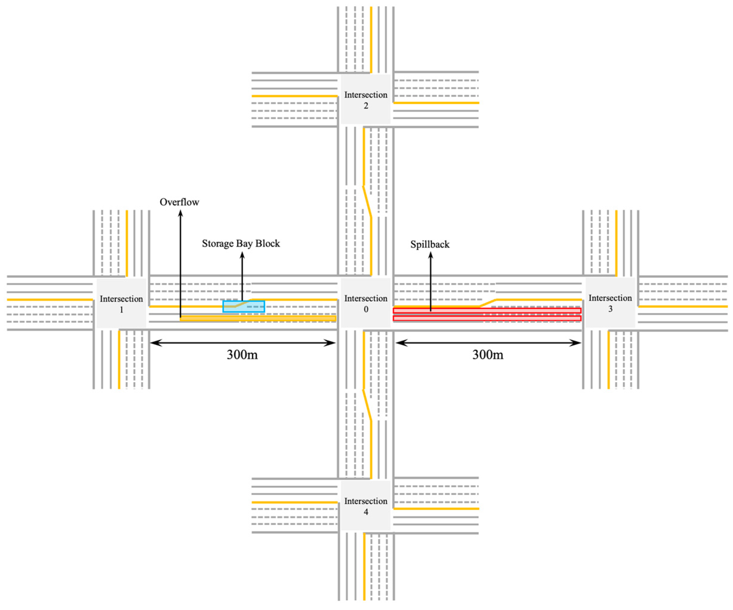
Using Vissim software to simulate oversaturated traffic, the motion data of vehicles under oversaturated traffic conditions can be obtained [34]. In this paper, by controlling the value of the traffic input at the upstream intersection and the dissipative ability of the signal timing at the target intersection, designed 3 kinds of oversaturation: residual queues due to excessive traffic flow, overflow of the storage bay, and overflow of the downstream intersection. The schematic diagram of the experimental design is shown in Figure 1.
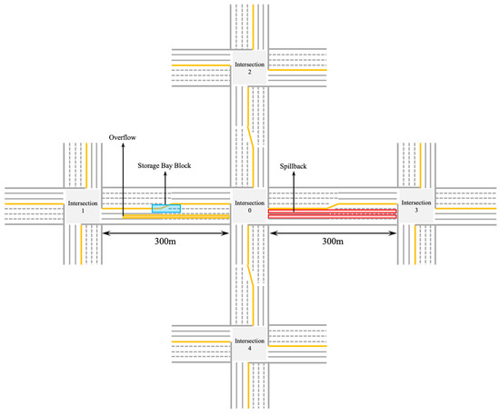
Figure 1.
Oversaturation traffic simulation design.
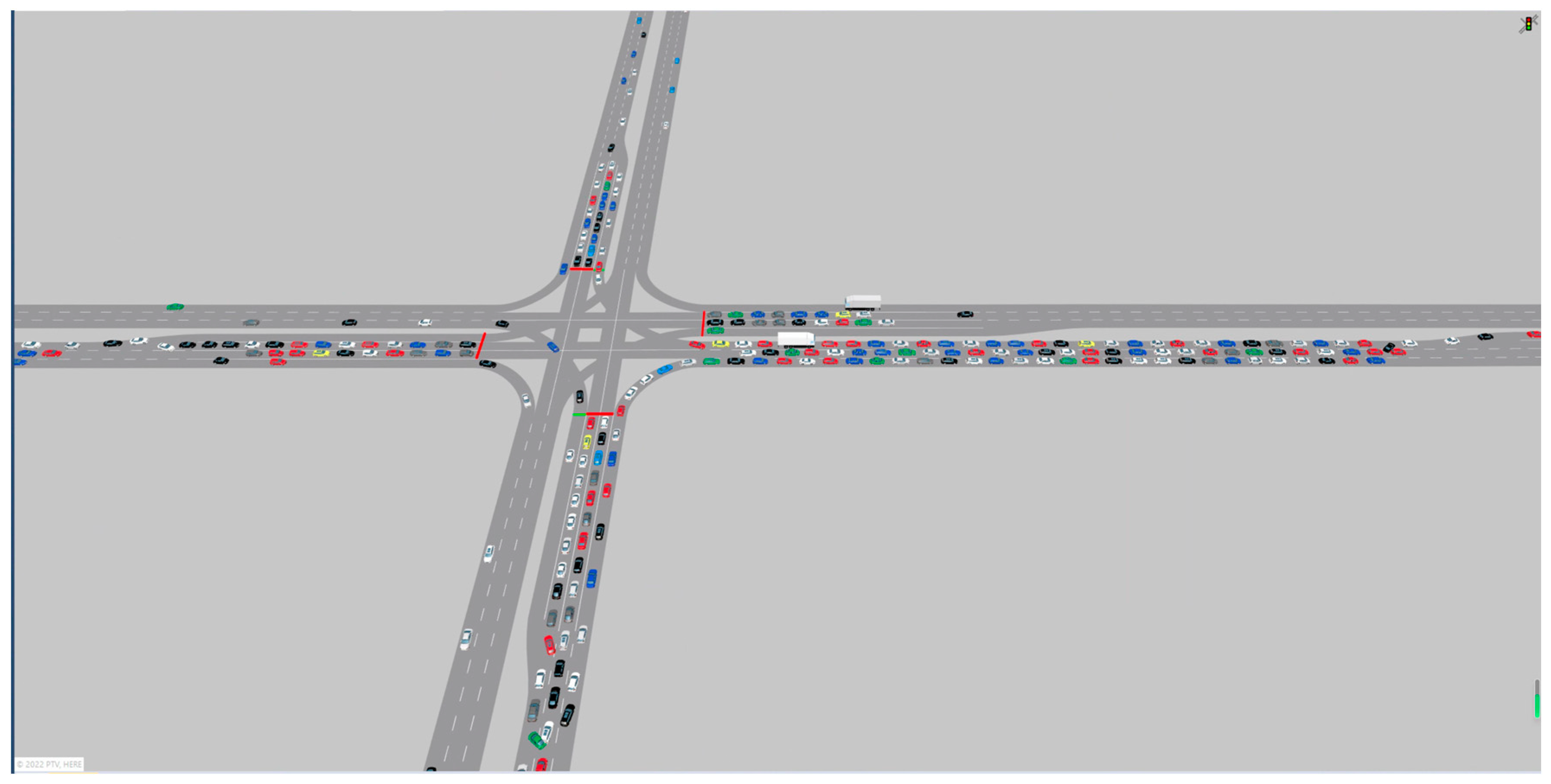
The Vissim oversaturation simulation software is shown in Figure 2. There are residual queues and overflows in the storage bay at the westbound, and the westbound is affected by the overflow at the east outlet. This paper will analyze the oversaturated traffic based on the simulation data in this scenario.
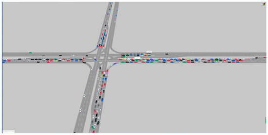
Figure 2.
Vissim Simulation of oversaturation in this paper.
2.2. Vehicle Formation
Vehicle formation refers to the formation of vehicles on the road into one or more objectives according to their position and speed, and each vehicle formation has its formation speed and density. The formation of discrete vehicles on the road is beneficial to the division of stop queues and other queues with different speeds and to improve the utilization of green time in the process of traffic signal control.
By counting from the stop line to its upstream, the position of a vehicle on a certain lane is denoted as , the corresponding speed of the vehicle is denoted as , and the head-to-head distance is . Consecutive vehicles with similar distances can be divided into a formation. If the speed of a vehicle can make it keep up with the formation ahead within a certain short , it can be considered that it belongs to the same formation as the vehicle ahead, and the conditions should be met:
should not be too large. It should be close to the unit green extension. This paper takes s.
As shown in Figure 3, assuming that the vehicles in the movement can be divided into m vehicle formations, and even single vehicle can also become a formation. It is denoted as , and with n vehicles is denoted as . If there is a vehicle in the movement, there must be at least .
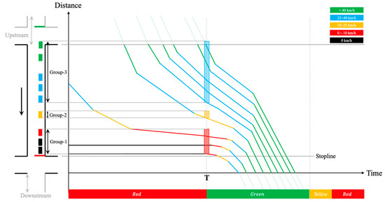
Figure 3.
Time–space diagram of vehicle formation.
Denoted the formation in front of a certain vehicle that has been classified into j vehicle as . If this vehicle belongs to the formation in front, it will be added to . Otherwise, the vehicle will become the first vehicle of the new formation, and the new formation will be added to of the movement. The formation of a certain vehicle is classified as follow:
Denoted the number of vehicles in a certain formation as . Formation is denoted as a whole, and the length of each vehicle is , then the position of the head of the formation is , and the tail is . The length of the formation can be calculated as follow:
Since the vehicle formation is compressible in space, set the minimum safe distance between vehicles as , then when all vehicles keep the minimum safe distance (), the minimum length of formation can be calculated as follow:
2.3. Virtual Detector
With the help of advanced traffic detection methods and multi-source perception, such as radar and video, and under the condition of known vehicle motion coordinates, virtual detectors can be flexibly set up in the detection area, which can achieve the same detection effect as traditional loop detectors. At the same time, it avoids negative effects such as damage to the road surface or signal interference.
The schematic diagram of the vehicle passing through the virtual detection area is shown in Figure 4. The blue part is the detection area. Assuming that there are n vehicles in the detection area, their positions are denoted as the corresponding set . The position of a certain virtual detector and the length of its detection area can be denoted as and . Its detection area is defined as , and the complete set of detection areas is , the corresponding detector state is a Boolean variable set .
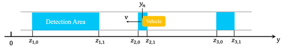
Figure 4.
The layout of virtual detectors.
When is in the corresponding detection area , the corresponding detector can be activated. In this way, the detector activated and inactivated pulse sequences are obtained, which are denoted as and . According to the information above, indicators such as traffic volume, occupancy rate, and headway can be calculated.
2.4. Quantitative Analysis of Oversaturation Degree
2.4.1. TOSI—Temporal Oversaturation Severity Index
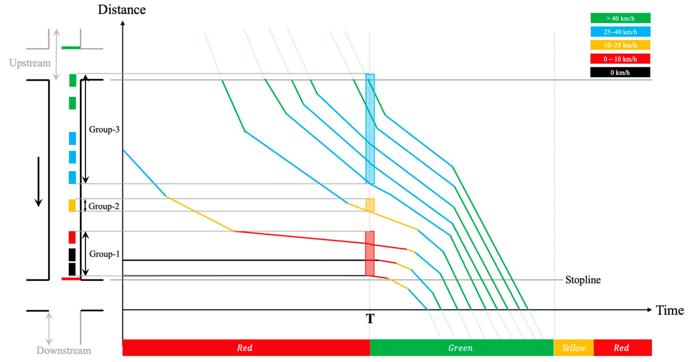
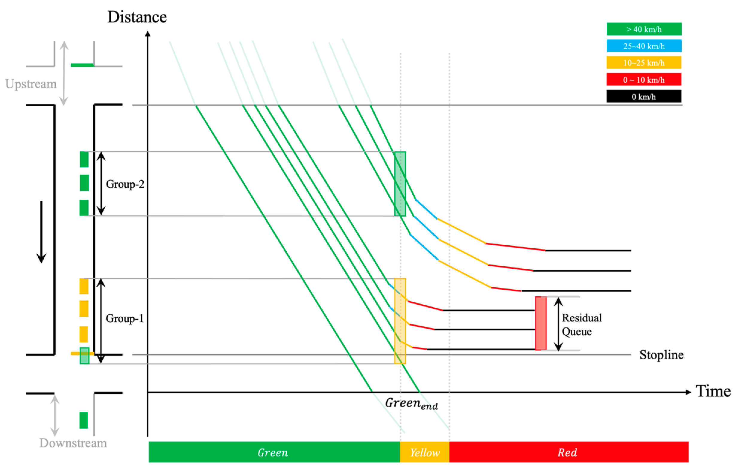
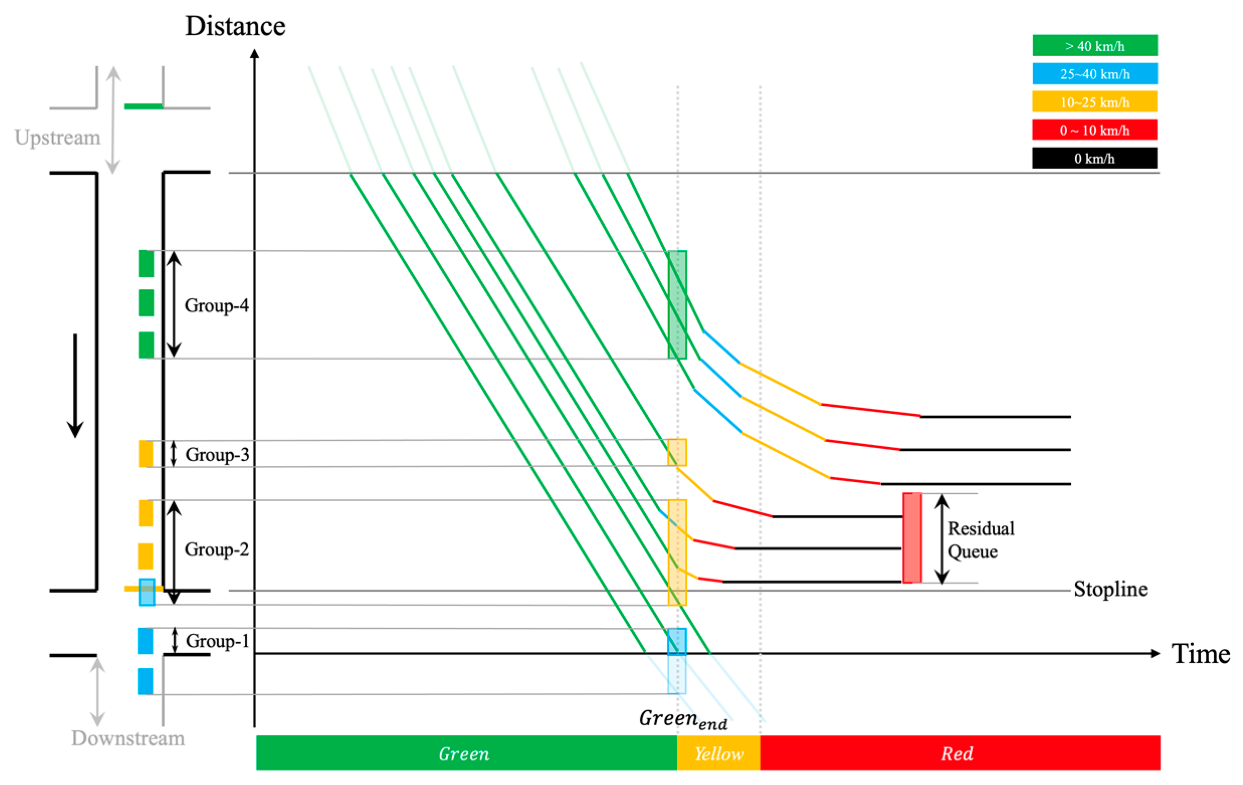
If the vehicles queuing up in the movement are not completely discharged at the end of the green time, which is shown in Figure 5, the residual queuing vehicles need to use the green time of the next cycle to pass the intersection. This green time reflects the degree of movement oversaturation in the temporal dimension. The ratio of it to the total green time is the temporal oversaturation severity index TOSI. TOSI > 0 means that the movement is oversaturated in temporal dimension due to the existence of residual queues. When TOSI > 1, it means that the residual queued vehicles cannot be completely dissipated within the green time of the next cycle, and two or more queue times occur.
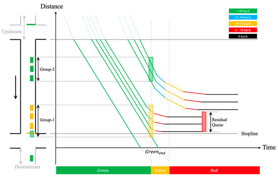
Figure 5.
Residual queue after the end of green time.
Different from the method of estimating the queue length according to the loop detector and the traffic shockwave theory and then calculating the TOSI, this paper calculates it according to the position of the vehicle formations. Denoted the moment of TOSI calculation as , and in the movement at , there are k vehicle formations, . Denoted the position of the stop line as . When TOSI exists, there is at least one formation that satisfies the constraints (the queue spans the stop line) .
Denoted that the speed set corresponding to each vehicle in the is , then the remaining number of vehicles that fail to pass the stop line and finally stop is:
Due to the discreteness of traffic flow in some cases (as shown in Figure 6), it is necessary to further determine the distance between the first vehicle in and the last vehicle of , and the average speed of . To judge whether the vehicles in belong to the residual queue, see as follows:
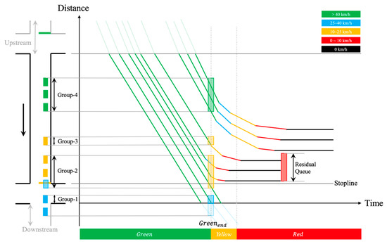
Figure 6.
Residual queue with discreteness of traffic flow after the end of green time.
In the equation set above, are the minimum distance threshold of the formation and the spatial average speed threshold. If or is smaller than its threshold, it can be considered that the vehicles belong to the residual queue. The final vehicle number of residual queue is .
TOSI is calculated as follows:
2.4.2. SOSI—Spatial Oversaturated Severity Index
When an overflow occurs at the downstream, vehicles at the upstream cannot pass through the intersection, even if they are in the green time, due to the spatial congestion caused by the overflow. The ratio of the unusable green time due to this reason, the total green time is the spatial oversaturation severity index SOSI, and SOSI > 0 reflects the spatial oversaturation degree of a certain movement.
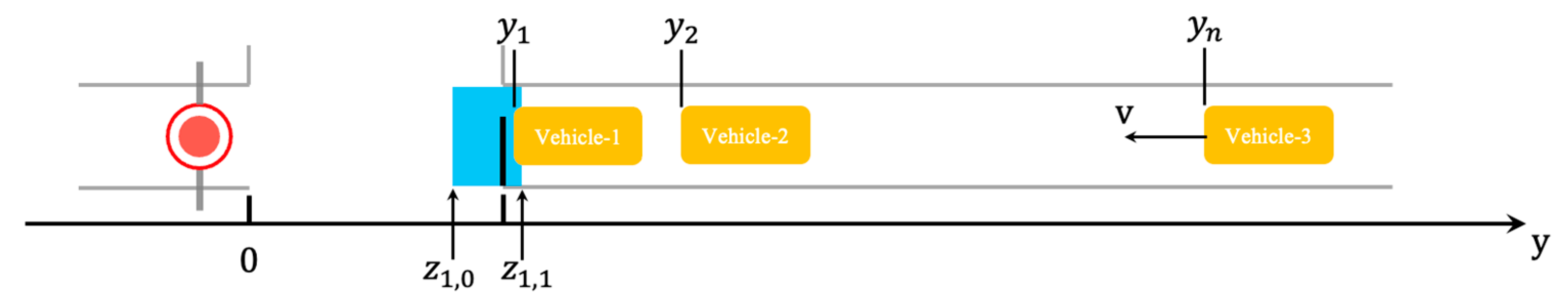
The calculation method of SOSI proposed in this paper relies on a stop-line detector. The layout of the detector should meet the following conditions:
- (a).
- When queuing, the first vehicle of the queued needs to activate the detector, but the subsequent vehicle cannot activate the detector; that is, , as shown in Figure 7;
 Figure 7. Detector layout requirements in queuing.
 - (b).
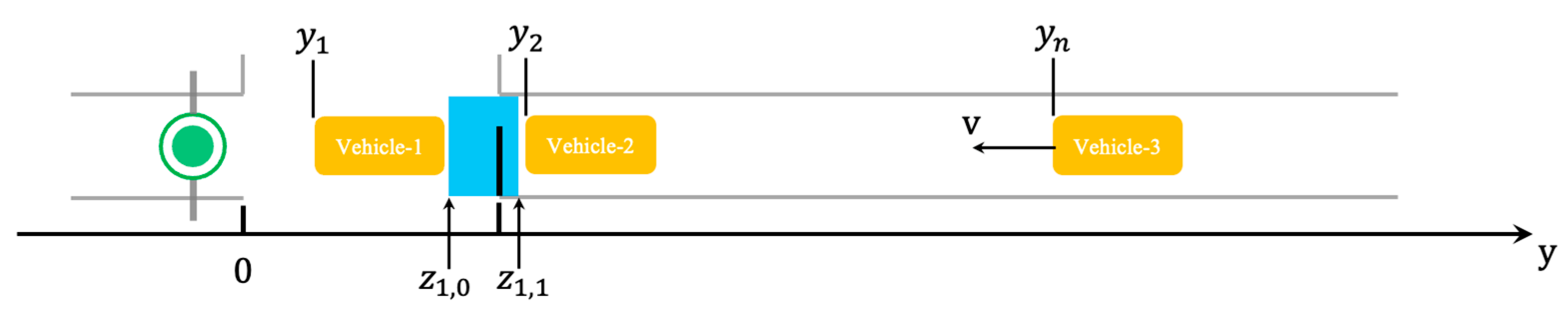
- When dissipating and the rear of the leading car leaving the detection area, the position of the head of the following car cannot make the detector active, that is: , as shown in Figure 8;
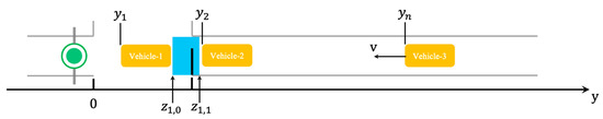 Figure 8. Detector layout requirements in dissipating.
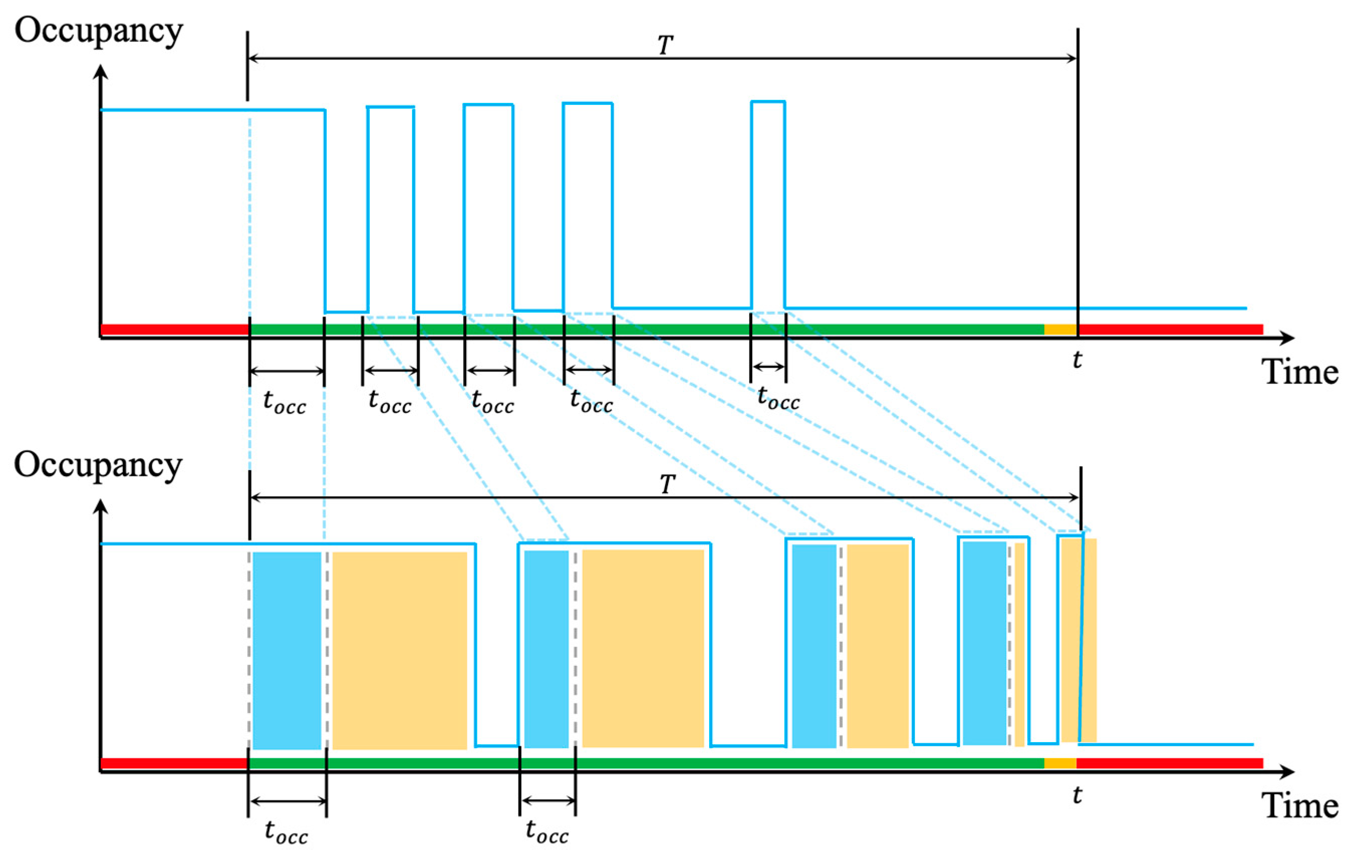
The number of activated and inactivated pulses (the blue line in Figure 9, activated is high and inactivate is low) in the statistical period are denoted as and , respectively, and the corresponding pulse response time series are denoted as and . The activated time a vehicle occupied when it passes through the detection area normally is denoted as (the blue shaded part in Figure 9), it is a dynamic value that depends on the speed of vehicle and the length of detection area. The detection period is from the beginning of green time to the end of yellow time ( and is the cycle length), and the span is . The value of SOSI is the sum of the time that exceeded the normally occupancy time (i.e., The sum of the yellow shaded part in Figure 9). The red, yellow, and green bar on the horizontal axis is a timing chart of the color change of the traffic signal lights.
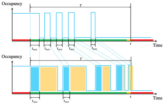
Figure 9.
Pulses of SOSI detectors in undersaturation and oversaturation traffic condition.
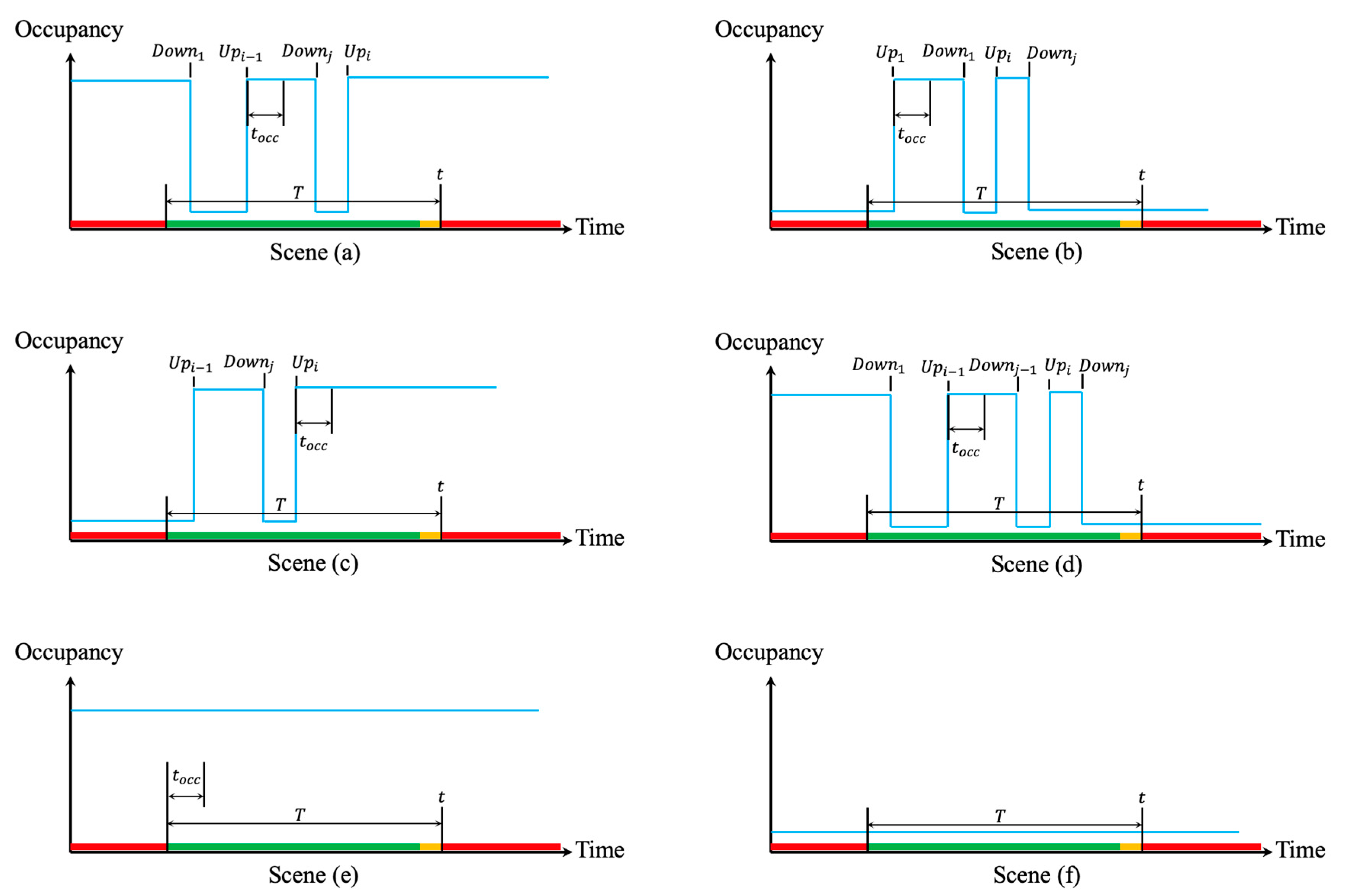
Under the detector layout described above, and according to the arrival and queuing conditions of the vehicle, the detector pulses in the statistical period can be divided into 6 scenes in Figure 10. The red, yellow, and green bar on the horizontal axis is a timing chart of the color change of the traffic signal lights, and the blue line is the value of the SOSI detector’s pulse (activated is high and inactivate is low). And the corresponding SOSI calculation methods are as follows.
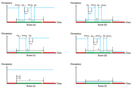
Figure 10.
Pulses of SOSI detectors in different scenes: (a) When the green light starts and there is a stop queue in stop line, the first vehicle can pass the stop line without being affected by the spillback, and after the green time, the last vehicle cannot pass the stop line due to spillback; (b) There is no stop queue before the green light starts and all vehicles can pass the stop line normally during the green time; (c) There is no stop queue before the green light starts but the last vehicles cannot pass the stop line due to spillback; (d) When the green light starts and there is a stop queue in stop line, all vehicles can pass the stop line normally during the green time; (e) When the green light starts and there is a stop queue in stop line, the first vehicle cannot pass the stop line even the green light becomes red due to spillback; (f) There is no stop queue before the green light starts and no vehicle passes the stop line during green time.
- (a).
- If and :
- (b).
- If and :
- (c).
- If :
- (d).
- If :
- (e).
- If and the detector is activated before the statistical period, but it never be inactivated during the statistical period;
- (f).
- If and the detector is inactivated before the statistical period, but it never be activated during the statistical period.
The SOSI of scenes (e) and (f) need to be considered in combination with the corresponding pulse response time series of the previous cycle statistics. Let the pulse response time series of all statistics before the statistical period be and , the number of their recorded time are and .
When at least one of the following conditions exists, then SOSI = 0:
- ;
- ;
- , and .
When at least one of the following conditions exists, then SOSI = 1:
- and ;
- , and .
2.5. Identification of Oversaturation Regime and Cause
2.5.1. Identification of Oversaturation Regime
When the number of vehicles in the movement is large, it may not be discharged completely in time during the green time, which will lead to the occurrence of temporal oversaturation and behave as a significant TOSI value.
When temporal oversaturation occurs, although some vehicles fail to leave the intersection during the green time, they can be completely dissipated in the next cycle, and the TOSI value will dissipate by itself after only one cycle. This situation is mainly related to the volatility of the input traffic volume from the upstream; that is, the input traffic volume from the upstream to a certain movement occasionally exceeds the dissipative capacity of this movement. At this time, this movement is in the loading regime of oversaturation, and if appropriate measures are taken, the oversaturation may not further aggravate and spread.
However, when the traffic volume which is input from the upstream to the movement, exceeds the dissipative capacity of this movement for several consecutive cycles, these inputs cannot be effectively dissipated during the green time of several consecutive cycles, showing continuous and significant TOSI, the degree of oversaturation begins to intensify at this time, and it is in the oversaturated operation regime.
When the input traffic volume from the upstream to the movement begins to decrease, the vehicles in this movement are gradually dissipated. At this time, although there is still a continuous TOSI value, there has been a significant decline compared to the previous TOSI. The oversaturation is now in the recovery regime.
Denoted the acceptable TOSI value as (take 35% in this paper), and if it exceeds this value, the TOSI might be high. Denoted as the end of green time, and the number of vehicles in a certain movement at is . Denoted the green time and saturation headway as and , when , it is considered that the number of vehicles in the movement is too large, and it cannot be completely dissipated after the green time of the next cycle. Denoted the occurrence of as an event . To sum up, according to the three characteristics of this movement at to identify the regime of the oversaturation:
- The value of TOSI;
- , the number of vehicles in this movement at ;
- Whether the event occur multiple times in consecutive cycles (this paper takes 2 or more occurrences in 4 cycles).
The conclusion is in Table 1.

Table 1.
Identification of oversaturated regime.
Case 6 in the table reflects that low and has not been dissipated completely for several consecutive cycles, and TOSI is low; theoretically, there is no corresponding traffic scene. Case 7 in the table reflects that low but is not dissipated completely in several consecutive cycles (appears alone), and TOSI is high; this case needs to be combined with SOSI value to be identified. If SOSI > 0 at this time, it means that overflow occurs at the downstream, so that even if there are few vehicles in the movement, it is still unable to pass the stop line, resulting in high TOSI, which often occurs in the oversaturated operation regime; if SOSI = 0 at this time, it occurs because there is an offset between the two intersections, which makes many vehicles approach the stop line when the green time is about to end, resulting in high TOSI. However, this situation often does not cause the aggravation of oversaturation and spread.
2.5.2. Analysis of the Cause of Oversaturation
As mentioned above, occasionally, when the inputs from the upstream exceed the dissipative capacity of a certain movement, a temporary oversaturation will occur, which will dissipate by itself in the next cycle. However, in this case, if the queued vehicles overflow out of the storage bay, in addition to the hidden danger of increased oversaturation in the movement, it may also block the storage bay, and cause phase starvation in the adjacent movement, then the degree of oversaturation will increase, even spread to other movements. Therefore, in addition to the overflow and spillback, the storage bay blocking is also an important reason for the loading, aggravation, and spread of oversaturation.
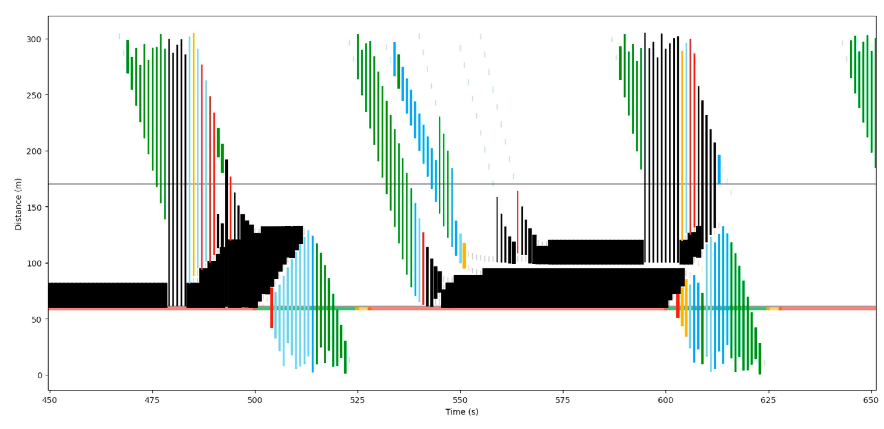
When a subsequently arriving vehicle on a movement is blocked outside the storage bay by vehicles overflowing from an adjacent movement, even if in the green time, there will be a growth queue in the upstream of the storage bay. As shown in Figure 11. In this figure, different color bars represent different vehicle formation groups, and the line is the trajectory of the vehicle, the darker the color, the slower the vehicle (Figure 12 is the same as Figure 11).
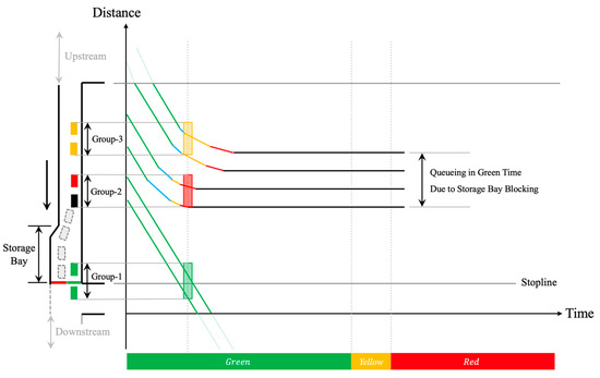
Figure 11.
Queue outside the storage bay due to the overflow from adjacent movement.
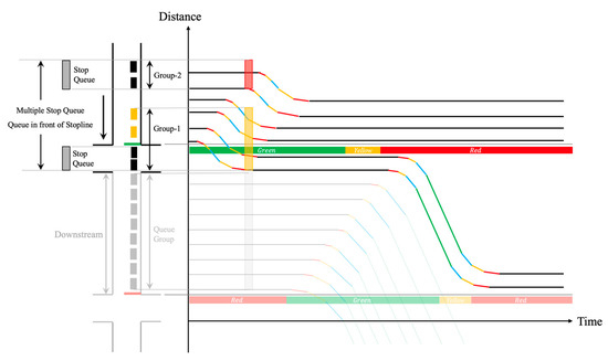
Figure 12.
Queuing due to spillback of downstream.
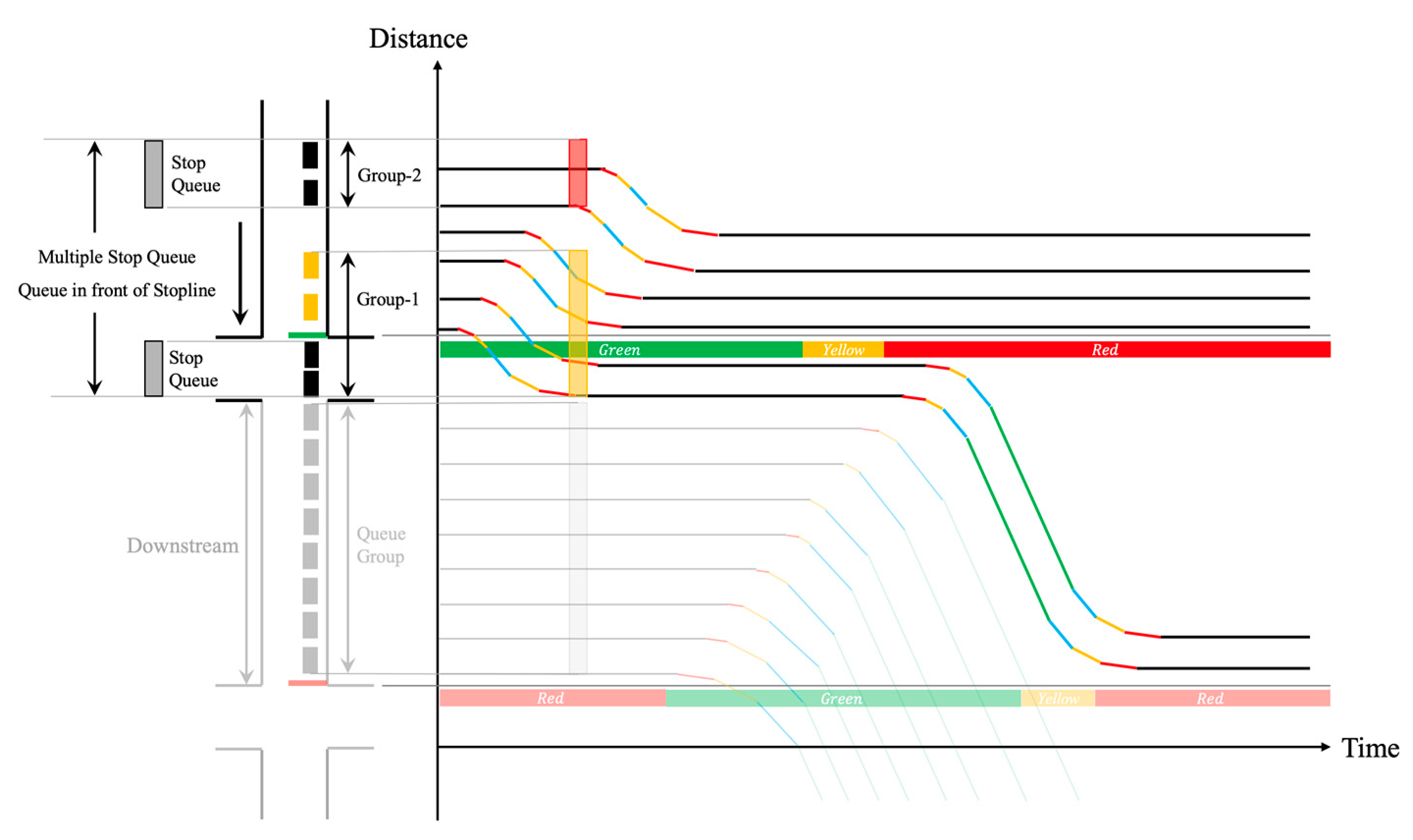
When a spillback occurs at the downstream, even if in the green time, there will be a growth queue in the downstream of the stop line. Even multiple formations of stop queues appear at the same time. As shown in Figure 12.
In the case of undersaturation and there is no overflow in the storage bay, if there are subsequent vehicles arriving, the maximum queue length of vehicles should reach the maximum value after a certain period when the green light starts; if no subsequent vehicles arrive, the maximum queue length should be equal to the queue length when the green time starts. There is no situation that “after the tail position of the stop queue in the upstream of stop line is less than the maximum queue length, the queue length increases again”.
To sum up, the characteristics of storage bay blocking and the spillback are as follows:
- (a).
- During the green time, the number of stop queues at is more than the number of stop queues at ;
- (b).
- During the green time, the length of a queue at is greater than the length of a queue at ;
During the green time, denoted the set of vehicle positions and corresponding speeds on the movement at as , . Denoted the stop queue set as , set a threshold , when the interval between vehicles is greater than this value, it is determined that there is another stop queue; otherwise, it will be classified into the front stop queue.
One of the following conditions can be determined as an abnormal stop queue:
- (a).
- The number of stop queues at is greater than the number of stop queues at :
- (b).
- If the number of stop queues at adjacent times is equal, the coordinate of the end of the queue at is greater than the coordinate of the end of the queue at :
The above judgment needs to be made during the green time, and there is at least one stop queue; the constraints are as follows:
To sum up, when there is no abnormal stop queue, if TOSI > 0, it is a temporary oversaturation caused by the residual queues (overflow in the movement) by excessive short-term traffic volume. When there is an abnormal stop queue, the cause of oversaturation is:
and are the positions of storage bay and stop line.
3. Results
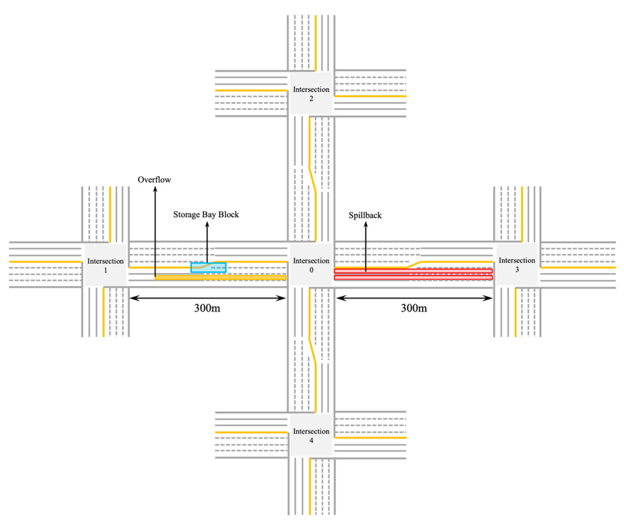
This paper used Vissim software for oversaturation simulation. The schematic diagram of the simulation design is shown in Figure 13. There are five intersections in the simulation, and Intersection 0 is the target intersection. Intersections 1~4 input vehicles periodically to Intersection 0 according to their traffic control signals. Taking the overflow and storage bay blocking in the westbound of Intersection 0, and the spillback from the westbound of Intersection 3 to Intersection 0 as an example, the analysis method of the oversaturation regimes is explained.
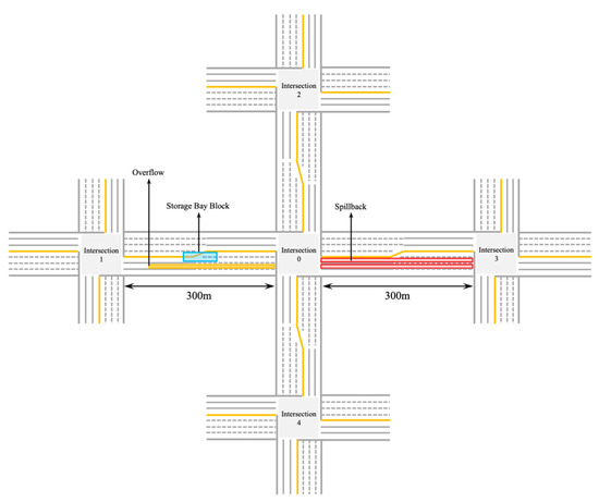
Figure 13.
Network of simulation.
The simulation time is 3600 s. From 0 s to 900 s, few vehicles are input to Intersection 0, and the indicators are analyzed under the condition of undersaturation. In 900 s~2700 s, increase the flow input from Intersections 1, make the westbound of Intersections 0 appear overflow and storage bay blocking, and increase the left turn and right turn at Intersections 2 and Intersections 4, respectively, so that there is a spillback from westbound of Intersections 3 to Intersections 0. From 2700 s, gradually reduce the flow input from Intersections 1~4 and observe the recovery of the oversaturation at Intersection 0.
3.1. Vehicle Formation and Virtual Detector
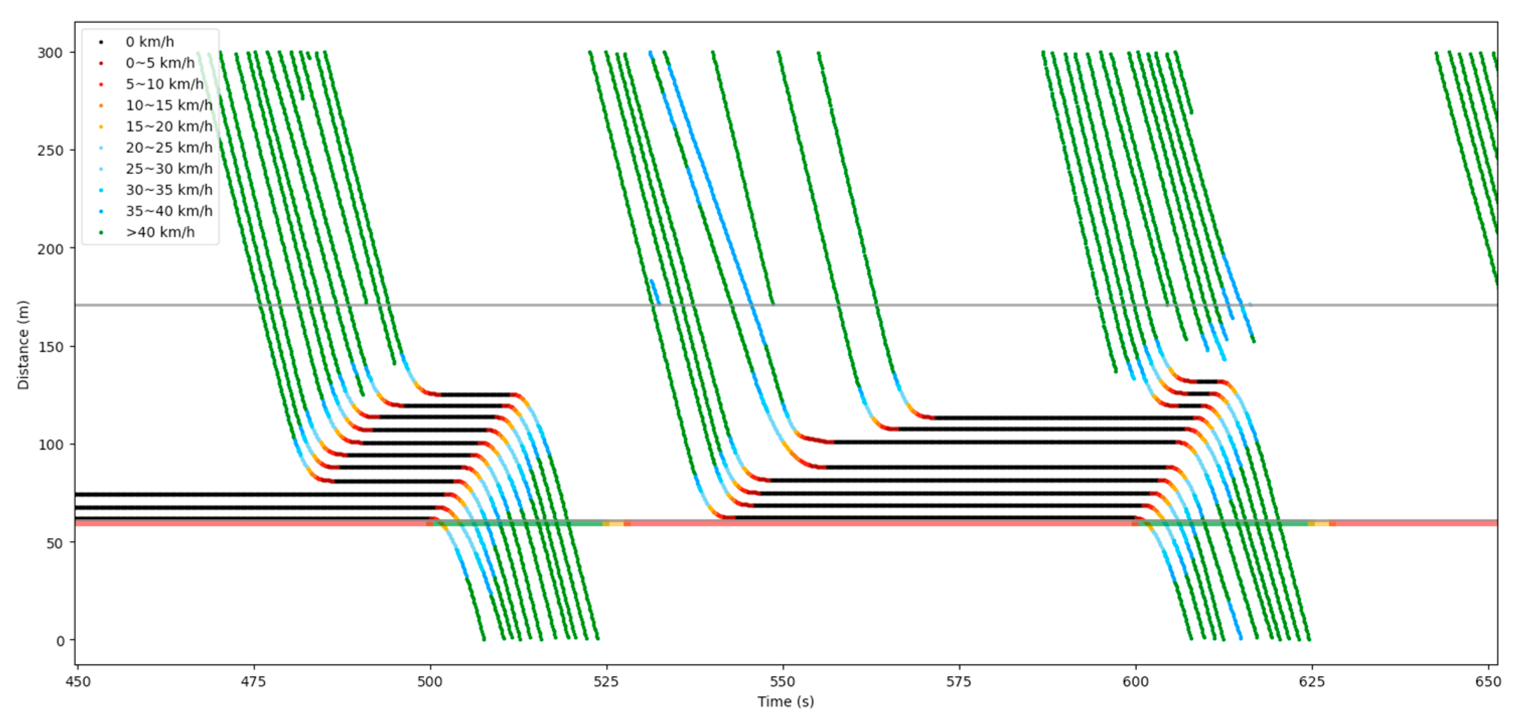
Figure 14 is a part of the space–time diagram of the trajectory of vehicles, each line is the trajectory of a corresponding vehicle. The different color lines in the figure represents the speed of each vehicle, the darker the color, the slower the vehicle, the speed values corresponding to each color are marked in the upper left corner of Figure 14. The position of the stop line is about 60 m (y = 60 in Figure 14, and the red, yellow, green of this line is the color change of the traffic signal lights in corresponding time), and the length of the storage bay is from 60 m to 170 m (the gray line in Figure 14). Some vehicles appear or disappear suddenly in this figure means that some vehicles drive in or out of the movement.

Figure 14.
A part of time–space diagram in simulation.
Figure 15 is the corresponding vehicle formation after the formation division of Figure 14, each vertical line is the queue of a corresponding vehicle formation. The different color vertical lines in the figure represents the speed of the vehicle formation, the darker the color, the slower the vehicle, the speed values corresponding to each color are marked in the upper left corner of Figure 14 (it should be noted that the black part represents the stop queue.). The thickness of each vertical line represents the density of the vehicle formation, and the length of the line represents the length of the vehicle formation. Since the speed of each vehicle in the movement is relatively independent, the distance between adjacent vehicles also changes accordingly, so the vehicle formation conforms to the dynamic change law presented in Figure 14.

Figure 15.
Corresponding vehicle formation of Figure 14.
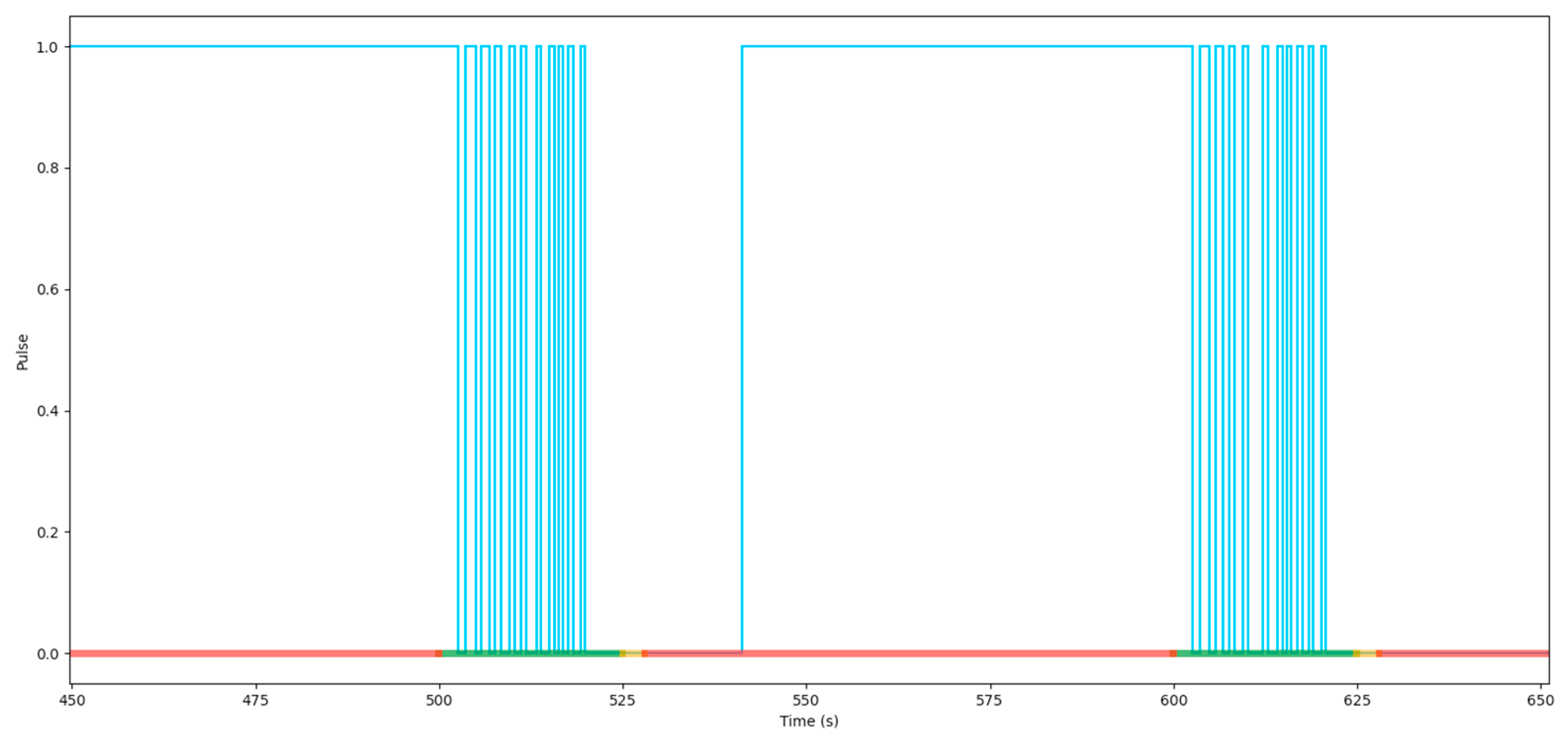
Figure 16 shows the corresponding pulses of the detector of Figure 14. The red, yellow, and green bar on the horizontal axis is a timing chart of the color change of the traffic signal lights. The position of the virtual detector is near the upstream of the stop line (about y = 61 m in Figure 14). The blue line in Figure 16 is the value of detector’s pulse. When the value of pulse is 1, it means that the detector is activated; 0 is inactivated on the contrary. SOSI can be calculated with the aid of this detector which accurately reflects the situation when the vehicle leaves the stop line during the green time.
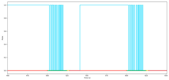
Figure 16.
Corresponding stop line virtual detector’s pulse of Figure 14.
3.2. Quantitative Analysis of Oversaturation
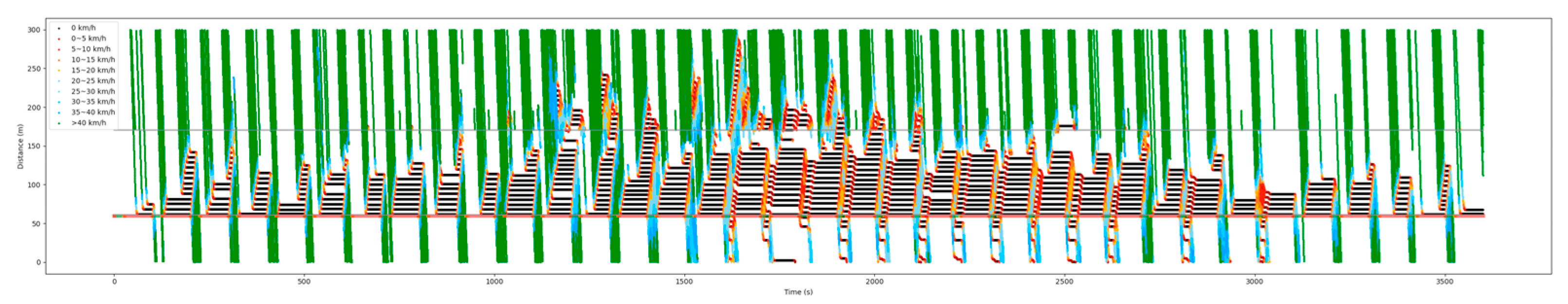
Figure 17 is the space–time diagram during the complete simulation. It reflects the trajectory of the vehicle in the movement, such as in Figure 14, but it is during the complete Vissim simulation. The darker the color and the denser the trajectories in this figure, the more serious the traffic congestion is.

Figure 17.
Time–space diagram of complete simulation.
Therefore, the evolution trend of traffic states can be seen in Figure 17. At the beginning of the simulation, the number of vehicles in the movement is small, but in a few cycles (fifth and eighth cycles), some vehicles approach the stop line at the end of the green time and lead to a residual queue, so there is a temporal oversaturation. However, the occurrence of the oversaturation is caused by the offset between the two intersections, so the oversaturation does not continue to the next cycle. When the traffic input at Intersections 1 and 4 is increased by 900 s, the dissipation capacity of the westbound at Intersection 0 cannot discharge these vehicles in time, and the degree of oversaturation in the temporal dimension begins to intensify. After several cycles, the vehicles on the westbound of Intersection 3 spillback to Intersection 0 and affected its straight westward flow, resulting in aggravation of spatial oversaturation. After 2000 s, the input from Intersection 1~4 decreased, and the westward straight flow of Intersection 0 began to dissipate slowly.
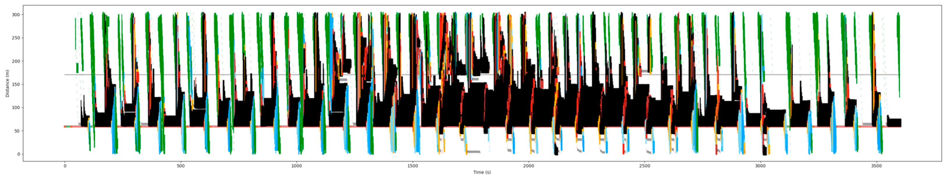
Figure 18, the corresponding vehicle formation figure of Figure 17, can reflect the vehicle formation division in the above time–space diagram to a certain extent (Like Figure 15 represents the vehicle formation of Figure 14). The black part is the vehicle formation which is stopped. The darker the color of the stop formation in the figure, the more serious the congestion is, and if the stop formation is discontinuous on the vertical axis, it means that there are multiple groups of parking queues at the same time. From the figure, the evolution of oversaturation from the beginning to the dissipation can be roughly seen, which preliminarily verifies the feasibility of quantifying the degree of oversaturation by vehicle formation.
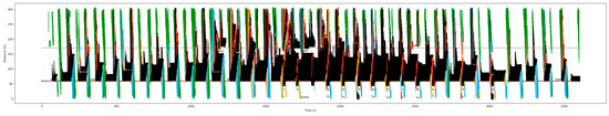
Figure 18.
Vehicle formation of complete simulation.
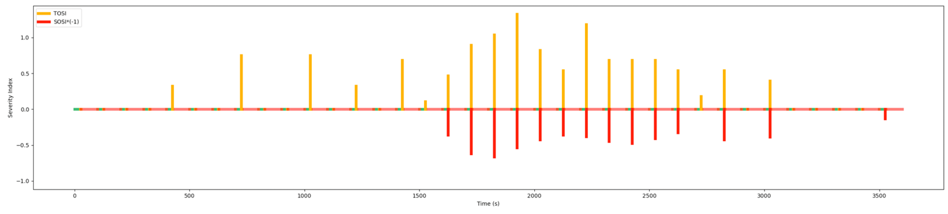
The degree of oversaturation calculated according to the vehicle formation is shown in Figure 19. In this figure, TOSI and SOSI show a process from low to high and then to low. The degree and change trend is consistent with the traffic conditions corresponding to the space–time diagram of the trajectory of the vehicle, the formation figure, and the simulation design, which verifies the accuracy of oversaturation quantification.
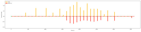
Figure 19.
Evolution of TOSI and SOSI.
3.3. Identification of Oversaturated Regimes
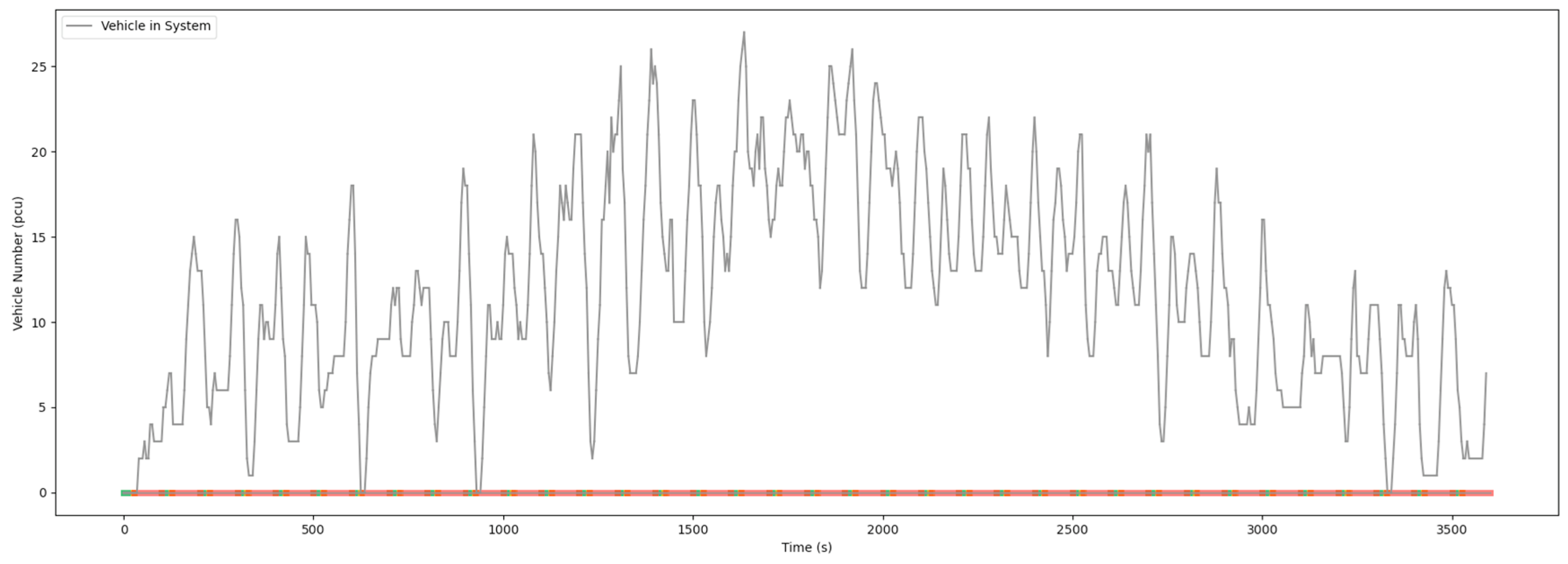
In the simulation, the green time for straight west at Intersection 0 is 25 s, and the saturated headway is 2.5 s. It can be calculated that when vehicles; there might be too many vehicles in this movement. And the change diagram of the number of vehicles in movement is shown in Figure 20.

Figure 20.
Number of vehicles in movement.
In the first 1000 s of the simulation, although some vehicles failed to pass the stop line during the green time, resulting in TOSI > , it dissipated by itself after only one cycle, and SOSI = 0, , which conforms to the description of Case 7 in Table 1.
From 1000 s to 1600 s, the number of vehicles in the movement has increased, and the oversaturation is still in the loading regime but not intensifying, which is in line with the descriptions of Cases 3 and 5 in Table 1. From 1600 s to 2700 s, the oversaturation began to intensify. and event occurred many times in a continuous cycle accompanied by TOSI > , as described in Case 1 in Table 1.
After 2700 s, the input from the upstream decreases, and the vehicles in the movement gradually dissipate and reduce, , the TOSI value decreases, and the event tends to be independent. The oversaturation in the movement is in the recovery regime, as described in Cases 2 and 4 in Table 1.
3.4. Analysis of Cause of Oversaturation
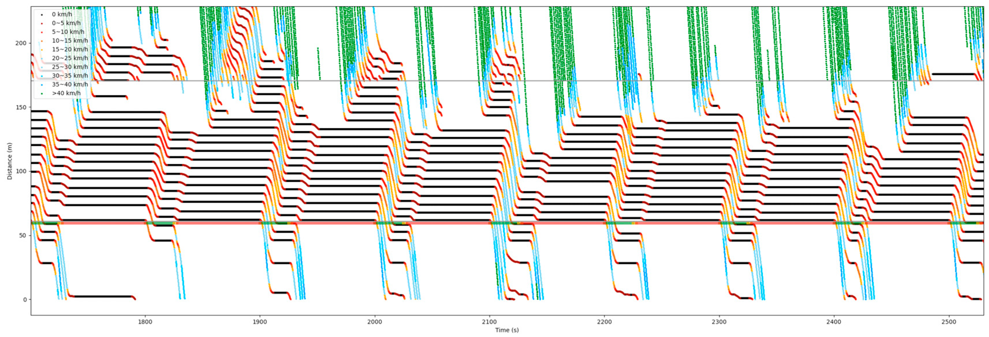
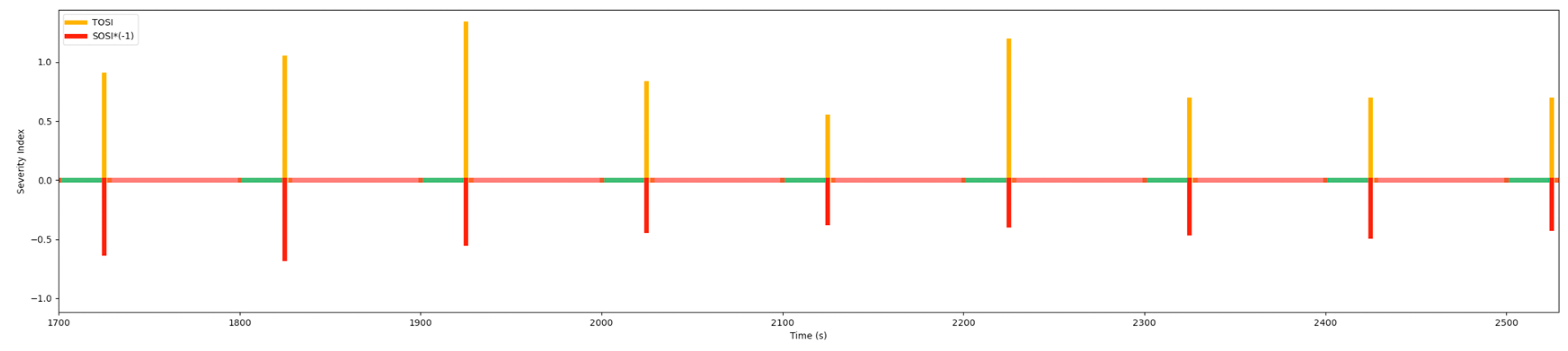
The oversaturated operation of the movement is intercepted for analysis. From Figure 21 and Figure 22, oversaturation occurs in temporal and spatial (i.e., spillback from downstream) dimensions simultaneously in this period, and there is overflow in the westbound.
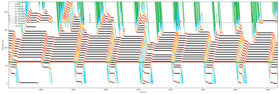
Figure 21.
Time–space diagram in oversaturation.
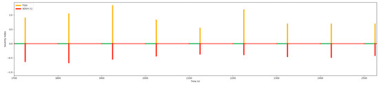
Figure 22.
Corresponding TOSI and SOSI of Figure 21.
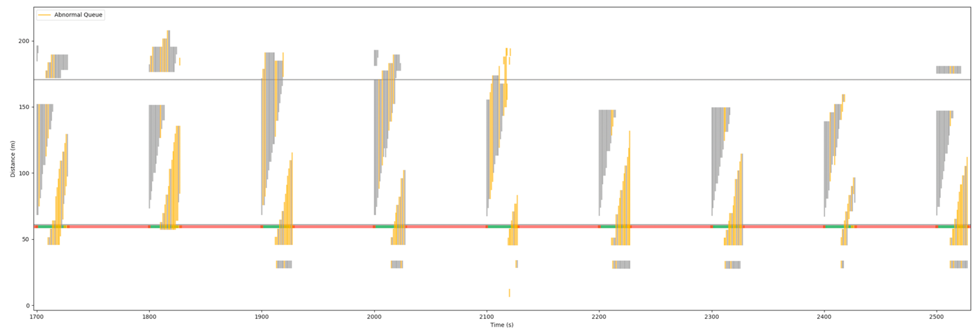
According to the analysis method of the causes of oversaturation in Section 2.5.2, the moment when there is an abnormal stop queue is represented by a yellow vertical line; otherwise, it is represented by a gray vertical line. The horizontal gray line (y is about 170) is the position of storage bay, and the horizontal colorful line (y is about 60 m, the position of stop line) represents the switching of the color of the signal light. When an abnormal queue occurs, if the abnormal conditions are determined to be the same at the next moment, it will be represented by a gray vertical line. That is, when determines that the abnormal stop queue has changed compared with the time , it is highlighted with a yellow line. It can be seen from Figure 23 that no matter whether the overflow comes from the downstream or the storage bay, it can be effectively identified, which is in line with expectations.
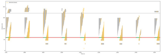
Figure 23.
Identification of abnormal queue in oversaturation.
4. Discussion
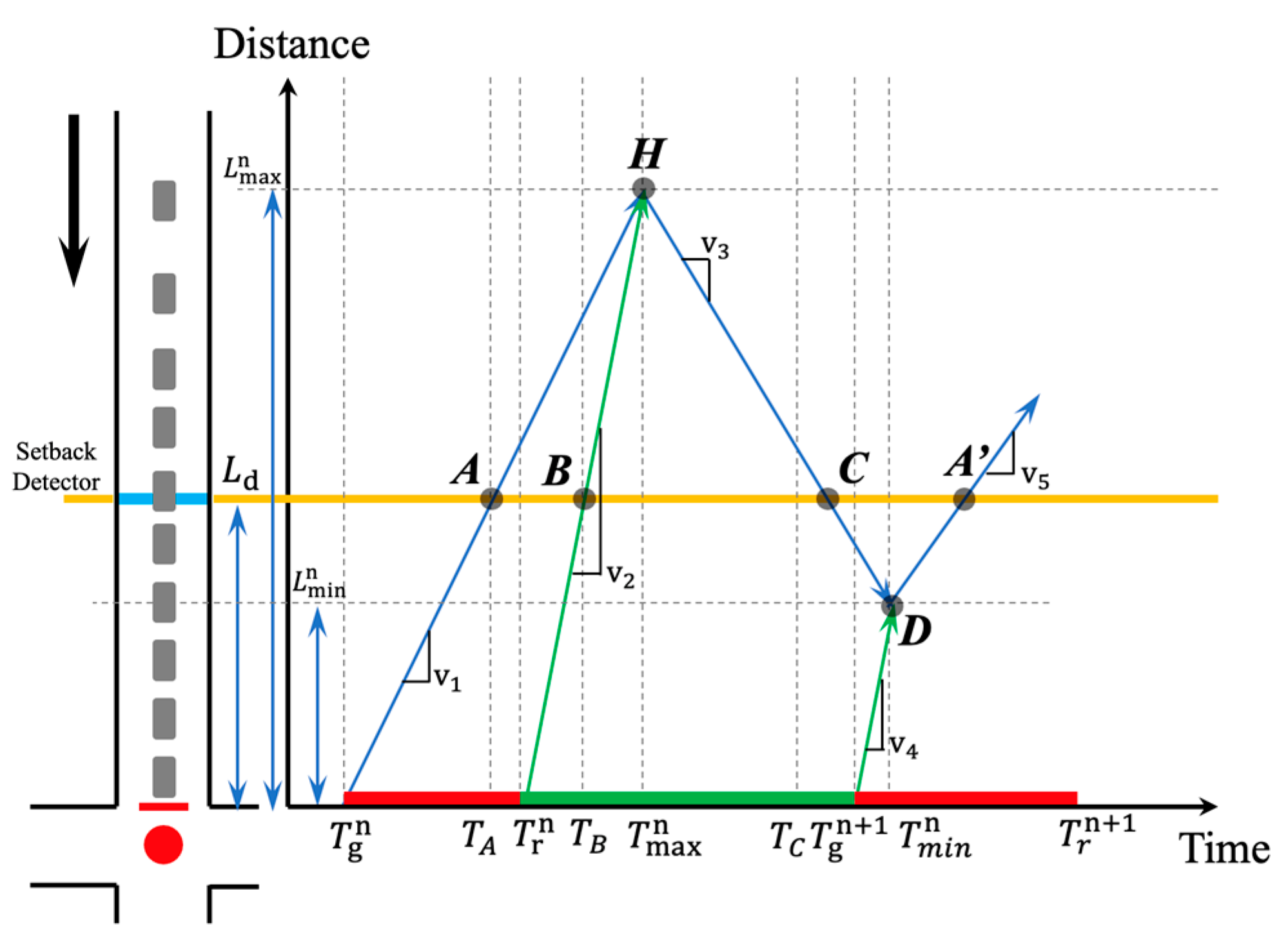
The existing TOSI calculation method relies on the high-resolution data obtained by the loop detector [21,22]. By setting a setback detector, the dissipation rate could be calculated according to the flow and density corresponding to the traffic state before and after . Then combined with the shockwave theory, TOSI could be calculated by estimating the residual queue length at point D in Figure 24. In this figure, the blue and green lines and their arrows represent the queuing growth and dissipation trends of vehicles, respectively. And the red dot on the left in Figure 24 indicates that the traffic signal light at the movement is red currently.
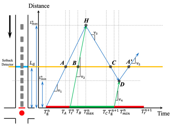
Figure 24.
Shockwave profile within a cycle.
In Figure 24, the arrival rate , the dissipation rate and need to be linearly fitted, which cannot fully match the arrival and dissipation rate of the actual traffic flow. There will be a certain error in the TOSI result calculated by this method.
In the comparison experiment, the green time is 25 s, calculated based on the saturated headway of 2.5 s, and a maximum of 10 vehicles can pass through the stop line during the green time. Therefore, the detector is set at 75 m upstream of the stop line (still within the storage bay). The residual queue length is estimated by this setback detector and then calculated TOSI.
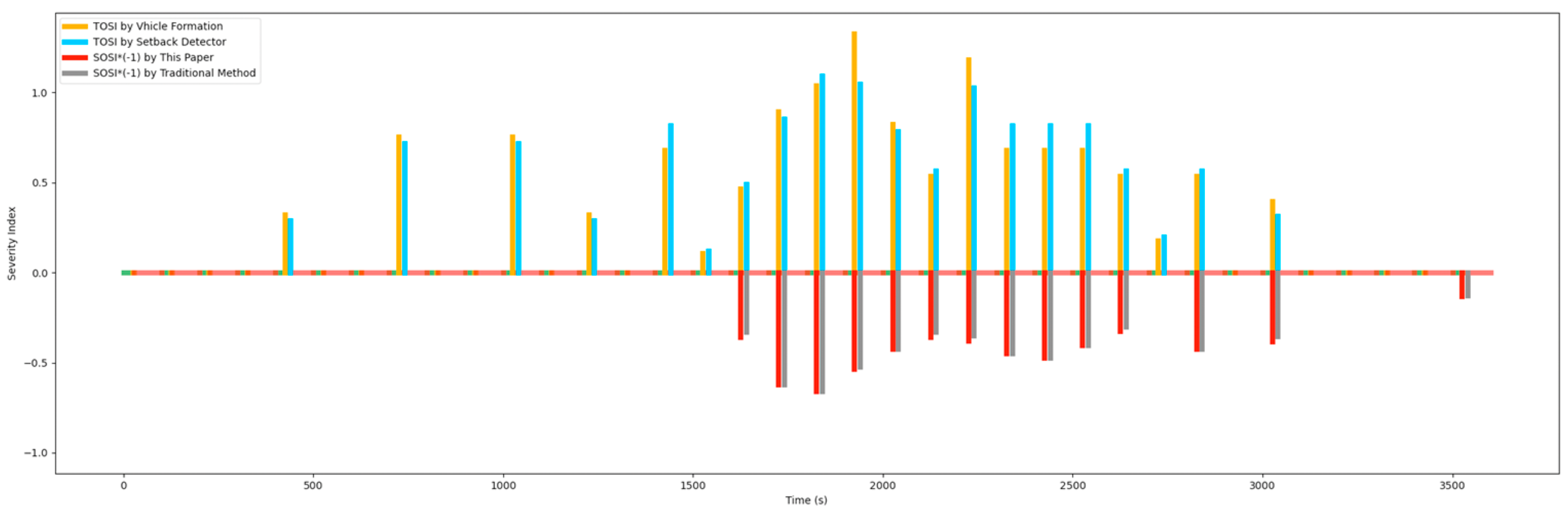
In Figure 25, it can be seen from the comparison results that the TOSI calculation method based on the vehicle formation proposed in this paper is relatively close to the results obtained by the traditional TOSI calculation method, which relies on a setback detector. The evolution trend of the oversaturation state reflected is the same. This further demonstrates the feasibility of using vehicle formations for TOSI calculations when multi-objective data are available.

Figure 25.
Comparison results of oversaturation severity index.
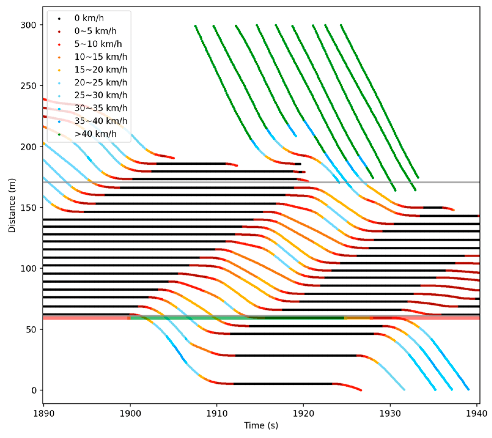
The main difference between the two methods is that in the case of downstream intersection spillback (SOSI > 0), if the estimated residual queue exceeds the setback detector’s position and occurs in multiple queues (TOSI > 1), the traditional method cannot obtain a more accurate residual queuing. In this paper, based on the data of multi-objective vehicles, the position and speed of each vehicle can be accurately known, and the vehicle formation can be obtained according to its position to obtain a more accurate residual queue length. Therefore, the calculated TOSI can more accurately reflect the degree of oversaturation in the temporal dimension. For example, at 1925 s of the simulation, the trajectory space-time diagram corresponding to the traffic state is shown in Figure 26. The TOSI calculated by the method in this paper was 1.34, while the value calculated by the traditional method was 1.06, as shown in Figure 25 where time is 1925. It can be seen from the time–space diagram that using multi-objective data to form vehicles to calculate TOSI can more accurately reflect the degree of oversaturation.
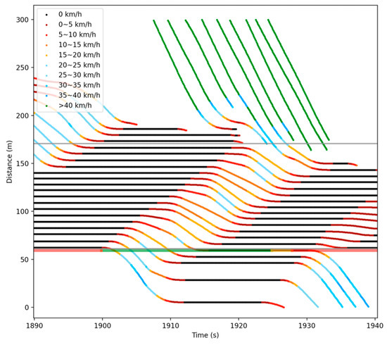
Figure 26.
Identification of abnormal queue in oversaturation (the trajectory space-time diagram corresponding to the traffic state).
The SOSI calculation in this paper is like the traditional method, and the comparison of the results also reflects the consistency of the conclusions of the two methods. In addition, this paper identified the regimes of oversaturation based on traffic volume and identified the cause of oversaturation based on abnormal queuing. In the follow-up work, we can further study the traffic control method under oversaturation according to the calculated oversaturation degree according to the regime and its cause.
Qin [35] built a traffic flow network model to investigate traffic congestion problems based on GPS trajectories. Though this method effectively identified the traffic congestion area and can help make decisions in traffic planning, it ultimately failed to provide specific quantitative results or parameters that could be directly used in traffic control, such as TOSI or SOSI. Tisljaric [36] proposed a method based on Speed Transition Matrix (STM) for traffic state estimation on a citywide scale using the novel traffic data representation. Though this method indicated the possible application for the traffic state estimation on macro- and micro-locations in the city area, it is still difficult to explain the extent and causes of traffic congestion or oversaturation such as the method this paper proposed.
5. Conclusions
The existing oversaturated traffic regime identification focuses on queue length or volume to capacity ratio, etc. When these indicators exceed a certain threshold, the traffic state is in a certain oversaturation regime, but the threshold does not form a unified standard. In addition, the existing oversaturated regime analysis is often based on loop detectors, and its detection accuracy has certain limitations. Based on the existing research, this paper analyzes the multi-objective data based on the advanced traffic detection methods, then quantifies the three oversaturation phenomena—residual queuing (overflow in movement), storage bay blocking, and spillback from temporal and spatial dimensions. Finally, combined with traffic volume analysis, a method for identifying the oversaturation regime is proposed, and the causes of oversaturation are identified based on abnormal growth queues, which can further determine the causes of oversaturation. The research objective of this paper is focused on the traffic movement in the intersection, which has certain reference significance for the in-depth research on the loading, oversaturated operation, and recovery of the oversaturated regimes. At the same time, the conclusions of this paper provide direct control parameters for the control strategy under the condition of traffic congestion, which can alleviate traffic congestion more accurately and achieve more efficient traffic operation efficiency and lower carbon emissions.
Author Contributions
Conceptualization, F.Z.; methodology, B.H. All authors have read and agreed to the published version of the manuscript.
Funding
This research received no external funding.
Institutional Review Board Statement
Not applicable.
Informed Consent Statement
Not applicable.
Data Availability Statement
The data presented in this study are available on request from the authors.
Conflicts of Interest
The authors declare no conflict of interest.
References
- Neufville, R.; Abdalla, H.; Abbas, A. Potential of connected fully autonomous vehicles in reducing congestion and associated carbon emissions. Sustainability 2022, 14, 6910. [Google Scholar] [CrossRef]
- Baghestani, A.; Tayarani, M.; Allahviranloo, M.; Gao, H.O. Evaluating the traffic and emissions impacts of congestion pricing in New York City. Sustainability 2020, 12, 3655. [Google Scholar] [CrossRef]
- Abdur-Rouf, K.; Shaaban, K. Measuring, mapping, and evaluating daytime traffic noise levels at urban road intersections in Doha. Qatar. Future Transp. 2022, 2, 625–643. [Google Scholar] [CrossRef]
- Hong, R.; Liu, H.; An, C.; Wang, B.; Lu, Z.; Xia, J. An MFD construction method considering multi-source data reliability for urban road networks. Sustainability 2022, 14, 6188. [Google Scholar] [CrossRef]
- González, S.S.; Bedoya-Maya, F.; Calatayud, A. Understanding the effect of traffic congestion on accidents using big data. Sustainability 2021, 13, 7500. [Google Scholar] [CrossRef]
- Padrón, J.D.; Soler, D.; Calafate, C.T.; Cano, J.-C.; Manzoni, P. Improving air quality in urban recreational areas through smart traffic management. Sustainability 2022, 14, 3445. [Google Scholar] [CrossRef]
- Wang, J.; Li, Y.; Zhang, Y. Research on carbon emissions of road traffic in Chengdu City based on a LEAP model. Sustainability 2022, 14, 5625. [Google Scholar] [CrossRef]
- Noaeen, M.; Mohajerpoor, R.; Far, B.H.; Ramezani, M. Real-time decentralized traffic signal control for congested urban networks considering queue spillbacks. Transp. Res. Part C Emerg. Technol. 2021, 133, 103407. [Google Scholar] [CrossRef]
- Sun, W.; Wang, Y.; Yu, G.; Liu, H.X. Quasi-optimal feedback control for an isolated intersection under oversaturation. Transp. Res. Part C Emerg. Technol. 2016, 67, 109–130. [Google Scholar] [CrossRef] [Green Version]
- Ding, H.; Guo, F.; Zheng, X.; Zheng, W. Traffic guidance–perimeter control coupled method for the congestion in a macro network. Transp. Res. Part C Emerg. Technol. 2017, 81, 300–316. [Google Scholar] [CrossRef]
- Mariotte, G.; Leclercq, L. Flow exchanges in multi-reservoir systems with spillbacks. Transp. Res. Part B Methodol. 2019, 122, 327–349. [Google Scholar] [CrossRef]
- Keyvan-Ekbatani, M.; Carlson, R.C.; Knoop, V.L.; Papageorgiou, M. Optimizing distribution of metered traffic flow in perimeter control: Queue and delay balancing approaches. Control. Eng. Pract. 2021, 110, 104762. [Google Scholar] [CrossRef]
- Mo, X.; Jin, X.; Tian, J.; Shao, Z.; Han, G. Research on the division method of signal control sub-region based on macroscopic fundamental diagram. Sustainability 2022, 14, 8173. [Google Scholar] [CrossRef]
- Kii, M.; Goda, Y.; Vichiensan, V.; Miyazaki, H.; Moeckel, R. Assessment of spatiotemporal peak shift of intra-urban transportation taking a case in Bangkok, Thailand. Sustainability 2021, 13, 6777. [Google Scholar] [CrossRef]
- Wu, A.; Yin, W.; Yang, X. Research on the Real-time Traffic Status Identification of Signalized Intersections Based on Floating Car Data. Procedia-Soc. Behav. Sci. 2013, 96, 1578–1584. [Google Scholar] [CrossRef] [Green Version]
- Lian, X.; Jiang, W. Traffic condition evaluation of urban trunk road. Mod. Transp. Technol. 2020, 17, 54–59. [Google Scholar]
- Wang, L.; Zhang, L.; Min, L.; Haibo, Z. Precise judging method study of intersection traffic state. Sci. Technol. Eng. 2016, 16, 290–295. [Google Scholar]
- Chen, Z.; Liu, X.; Wu, W.; Tang, S. Identification method of traffic state and its authenticity combined with signal control. J. Chongqing Jiaotong Univ. (Nat. Sci.) 2016, 35, 95–100. [Google Scholar]
- Xu, J.; Wei, J.; Shou, Y. Comprehensive evaluation of urban road traffic operation status based on game theory-cloud model. J. Guangxi Norm. Univ. Nat. Sci. Ed. 2020, 38, 1–10. [Google Scholar]
- Zhang, L.; Wang, L.; Pan, K.; Li, Z. Intersection traffic state distinguish method based on comprehensive projection. J. Transp. Syst. Eng. Inf. Technol. 2016, 16, 83–91. [Google Scholar]
- Yao, J.; Tang, K. Cycle-based queue length estimation considering spillover conditions based on low-resolution point detector data. Transp. Res. Part C Emerg. Technol. 2019, 109, 1–18. [Google Scholar] [CrossRef]
- Cheng, Q.; Liu, Z.; Guo, J.; Wu, X.; Pendyala, R.; Belezamo, B.; Zhou, X. Estimating key traffic state parameters through parsimonious spatial queue models. Transp. Res. Part C Emerg. Technol. 2022, 137, 103596. [Google Scholar] [CrossRef]
- Yuan, S.; Zhao, X.; An, Y. Identification and optimization of traffic bottleneck with signal timing. J. Traffic Transp. Eng. Engl. Ed. 2014, 1, 353–361. [Google Scholar] [CrossRef] [Green Version]
- Aljamal, M.A.; Abdelghaffar, H.M.; Rakha, H.A. Estimation of traffic stream density using connected vehicle data: Linear and nonlinear filtering approaches. Sensors 2020, 20, 4066. [Google Scholar] [CrossRef]
- Gazis, D.C.; Potts, R.B. The Oversaturated Intersection; Highway Safety Research Institute: London, UK, 1963. [Google Scholar]
- Abu-Lebdeh, G.; Benekohal, R.F. Signal Coordination and Arterial Capacity in Oversaturated Conditions. Transp. Res. Rec. J. Transp. Res. Board 2000, 1727, 68–76. [Google Scholar] [CrossRef]
- Abu-Lebdeh, G.; Benekohal, R.F. Design and evaluation of dynamic traffic management strategies for congested conditions. Transp. Res. Part A 2003, 37, 109–127. [Google Scholar] [CrossRef]
- Roess, R.P.; Prassas, E.S.; McShane, W.R. Traffic Engineering; Pearson Education, Inc.: Upper Saddle River, NJ, USA, 2004. [Google Scholar]
- Lieberman, E.B.; Messer, C.J. Internal Metering Policy for Oversaturation Networks; Transportation Research Board: Washington, DC, USA, 1992. [Google Scholar]
- National Academies of Sciences, Engineering, and Medicine. Operation of Traffic Signal Systems in Oversaturated Conditions; Final Report; The National Academies Press: Washington, DC, USA, 2014; Volume 2. [Google Scholar] [CrossRef]
- Qian, Z.; Xu, J. Identification of oversaturated traffic conditions based on loop detection. J. South China Univ. Technol. Nat. Sci. Ed. 2013, 41, 99–104. [Google Scholar]
- Wu, X.; Liu, H.X.; Gettman, D. Identification of oversaturated intersections using high-resolution traffic signal data. Transp. Res. Part C Emerg. Technol. 2010, 18, 626–638. [Google Scholar] [CrossRef]
- Morozov, V.; Iarkov, S. Formation of the traffic flow rate under the influence of traffic flow concentration in time at controlled intersections in Tyumen, Russian Federation. Sustainability 2021, 13, 8324. [Google Scholar] [CrossRef]
- Wang, F.; Gu, D.; Chen, A. Analysis of traffic operation characteristics and calculation model of the length of the connecting section between ramp and intersection. Sustainability 2022, 14, 629. [Google Scholar] [CrossRef]
- Qin, J.; Mei, G.; Xiao, L. Building the traffic flow network with taxi GPS trajectories and its application to identify urban congestion areas for traffic planning. Sustainability 2021, 13, 266. [Google Scholar] [CrossRef]
- Tišljarić, L.; Carić, T.; Abramović, B.; Fratrović, T. Traffic state estimation and classification on citywide scale using speed transition matrices. Sustainability 2020, 12, 7278. [Google Scholar] [CrossRef]


Publisher’s Note: MDPI stays neutral with regard to jurisdictional claims in published maps and institutional affiliations. |
© 2022 by the authors. Licensee MDPI, Basel, Switzerland. This article is an open access article distributed under the terms and conditions of the Creative Commons Attribution (CC BY) license (https://creativecommons.org/licenses/by/4.0/).