
Spatial Differences and Influencing Factors of Industrial Green Total Factor Productivity in Chinese Industries


Abstract
:1. Introduction
2. Literature Review
3. Research Methodology
3.1. GML Index
3.2. Dagum Gini Coefficient
3.3. GTWR (Spatial-Temporal Weighted Regression Model)
4. Variable Specification and Data
4.1. Input-Output
- (1)
- Capital stock. We use the fixed assets value of industrial enterprises to represent the capital stock. There are no direct data of depreciation rate and fixed asset investment in the statistical yearbooks, but China’s Industry Statistical Yearbook provides the amount of accumulated depreciation. The depreciation rate (δit) is measured by the ratio of current year’s depreciation to last year’s fixed asset value, where the current year’s depreciation equals the current year’s accumulated depreciation minus the previous year’s accumulated depreciation. The fixed assets investment sequence is calculated by the difference between the current year’s fixed assets value and the last year’s fixed assets value. Finally, the industrial value-added series and fixed asset investment series (Iit) are deflated by the industrial producer price index and fixed asset investment price index, and uniformly converted into 2002 constant prices. The capital stock is estimated using the perpetual inventory method:where and respectively represent the capital stock in year t and year t − 1 in region i; is the depreciation rate in year t and region i; and is the capital input in year t and region i.
- (2)
- Labor input. Under normal circumstances, labor input refers to the actual number of workers engaged in a production process and their average time of labor service. This paper uses the average employment of industrial enterprises above a designated size (with operating revenue more than CNY 20 million) as a proxy variable of labor input.
- (3)
- Energy consumption. The energy input is measured by total amount of coal and other fossil energy used.
- (4)
- Expected output. We choose industrial value added as the expected output in the production process and adjust it to 2002 constant prices.
- (5)
- Undesired output. Industrial production generates a large amount of industrial waste, which will pollute the environment. Meanwhile, a large amount of carbon dioxide generated in the industrial production process will also harm the atmosphere. Therefore, we choose industrial sulfur dioxide emissions and carbon emissions as undesirable outputs. Following related studies [6,40,41], we select the fossil energy consumption and emission coefficient publicized in the Official Database of China (CEADs) and measured by the IPCC sub-sector emission accounting method as the proxy variable of carbon emissions.
4.2. Influencing Factors
- (1)
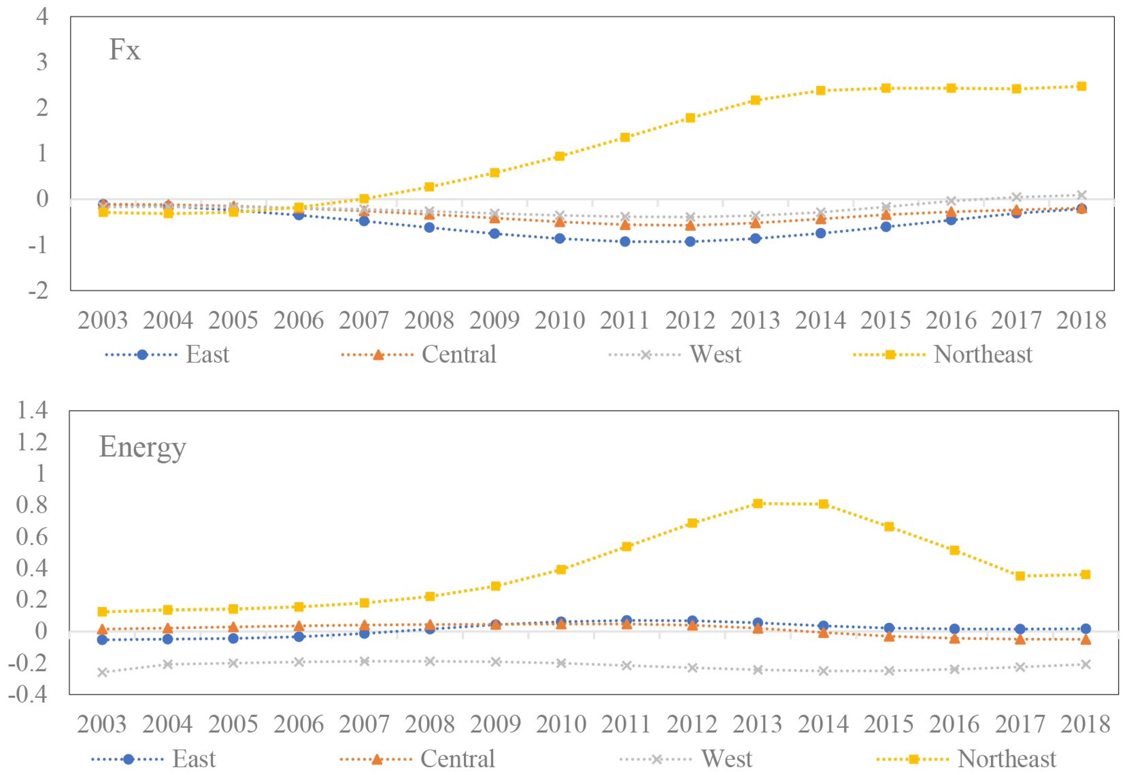
- Factor supply. The influence of factor supply on industrial GTFP regional differences is analyzed via the effect of capital and energy input. Capital input (Fx) is measured by the ratio of fixed capital input of industrial enterprises to GDP in that year. Energy structure (Energy) is measured by the ratio of coal consumption to total energy consumption.
- (2)
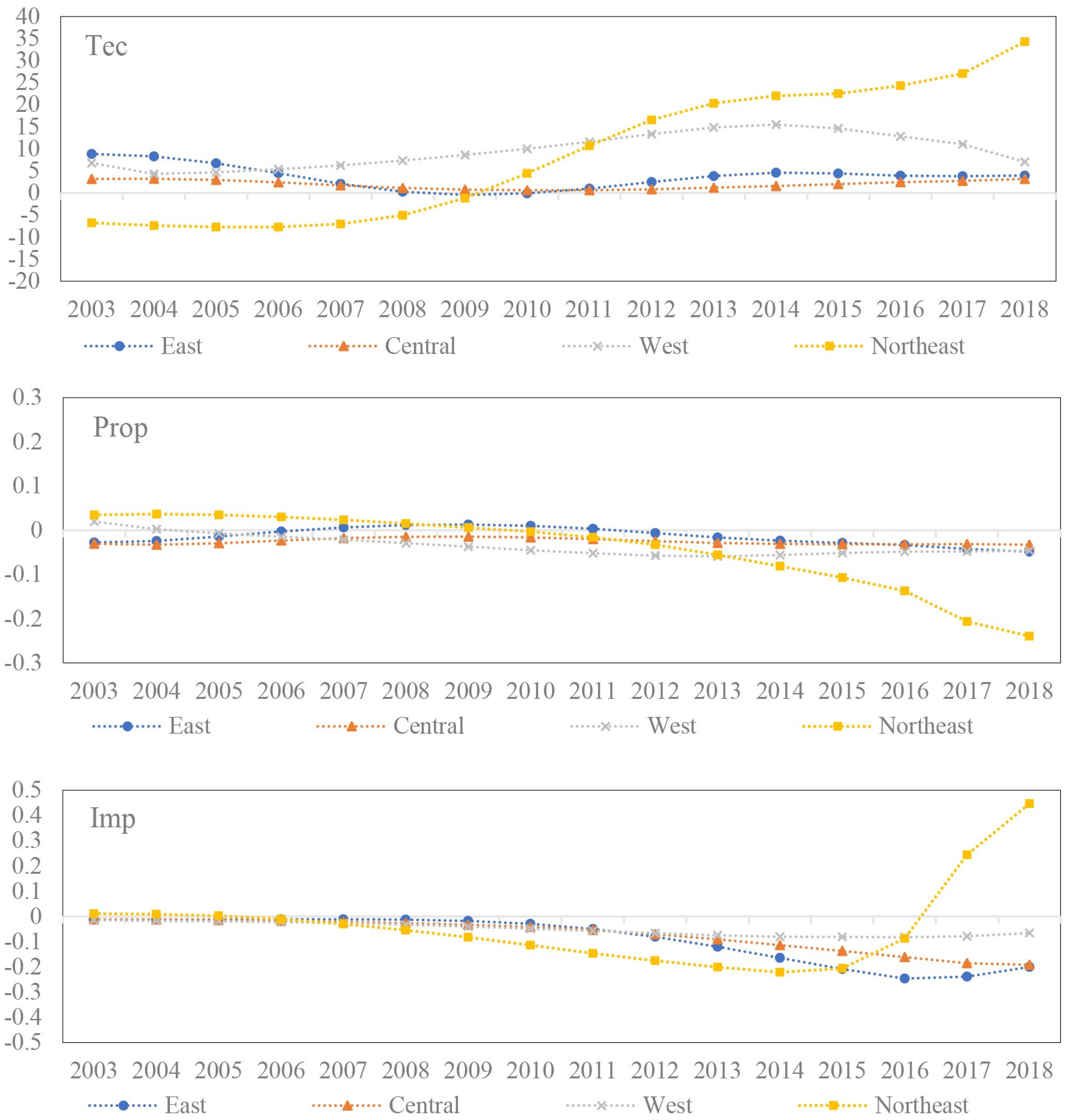
- Technological progress. We analyze the impact of technological progress on GTFP at three levels: R&D investment (Tec), measured by internal R&D expenditure as a percentage of GDP; patent applications (Prop), measured by the log of patent applications made by industrial enterprises above a designated size with a lag of one year; and technical modification and transformation (Imp), measured by the ratio of total funds devoted to technology introduction, adaptation, and absorption, and other aspects to GDP of industrial enterprises above regional scale, which also reflects the degree of industrial enterprises’ foreign technology dependence in this region.
- (3)
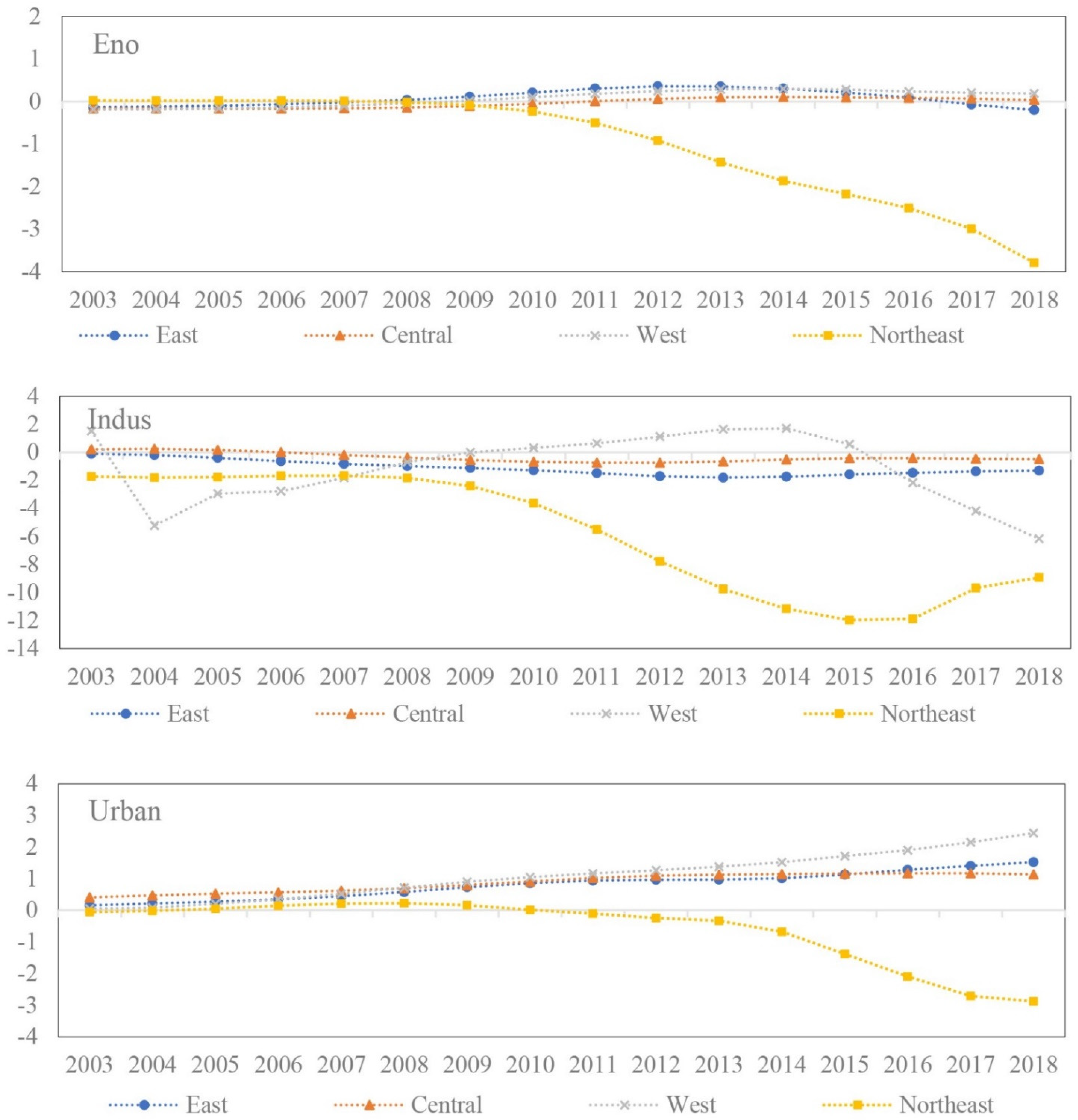
- Structural factors. The influence of structural factors on industrial GTFP is analyzed in three dimensions. First is the urban environmental governance level (Eno), measured by the proportion of investment in local industrial pollution control to GDP. Second is the agglomeration (clustering) level (Indus), measured by the location quotient index, which is calculated as follows:where and represent the number of employees of industrial enterprises above a designated size in region i at time t and the total number of employees in region i at time t. and represent the employment of China’s industrial enterprises and national total employment at time t. The larger the value of , the higher the agglomeration degree of industrial enterprises in this region. Thirdly, the urbanization level (Urban) measures the urbanization rate. A higher level of urbanization can bring more labor force to enterprises and is particularly conducive to attracting high-tech talents and promoting industrial development.
- (4)
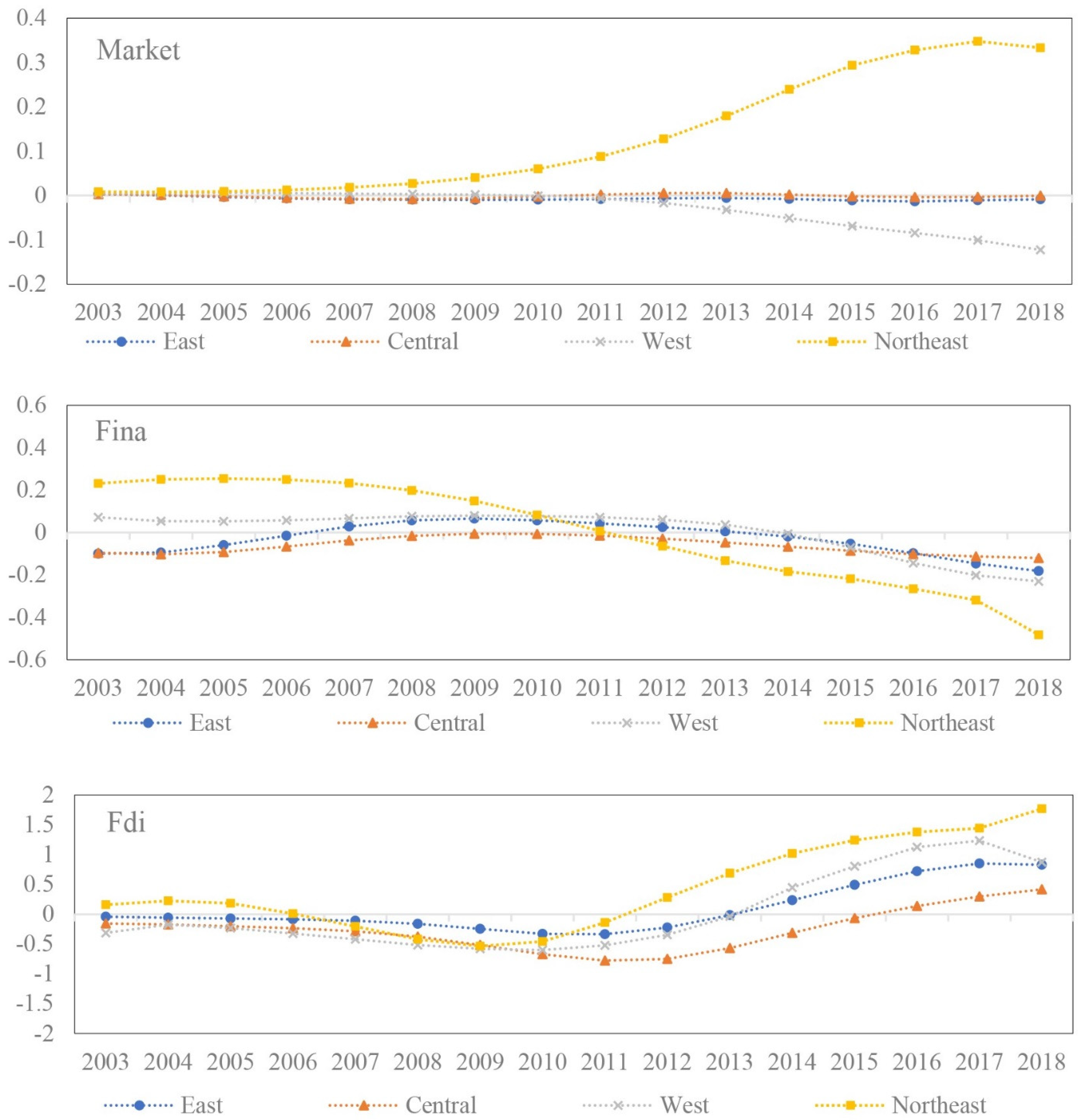
- Market environment. The influence of the market environment on GTFP is analyzed in three dimensions. First, the degree of marketization (Market). The marketization level plays an important role in stimulating market vitality and optimizing resource allocation efficiency. We adopt the marketization index from the research report “China’s Marketization Index—NERI Index of Marketization of China’s Provinces 2018 Report” to analyze the dynamic impact of the degree of marketization reform on GTFP in different regions. To remedy data deficiency, we reckoned the marketization index of 2017 and 2018 by the growth rate of the previous three years. In addition, industrial development cannot go without the provision of capital and financing. We analyze the spatial-temporal heterogeneity of the impact of capital investment on industrial GTFP from the perspective of regional financial development and foreign direct investment. Financial development (Fina) is measured by the ratio of outstanding loans of financial institutions to GDP. Foreign direct investment (FDI) is measured by the ratio of total foreign investment to GDP.
5. Empirical Analysis
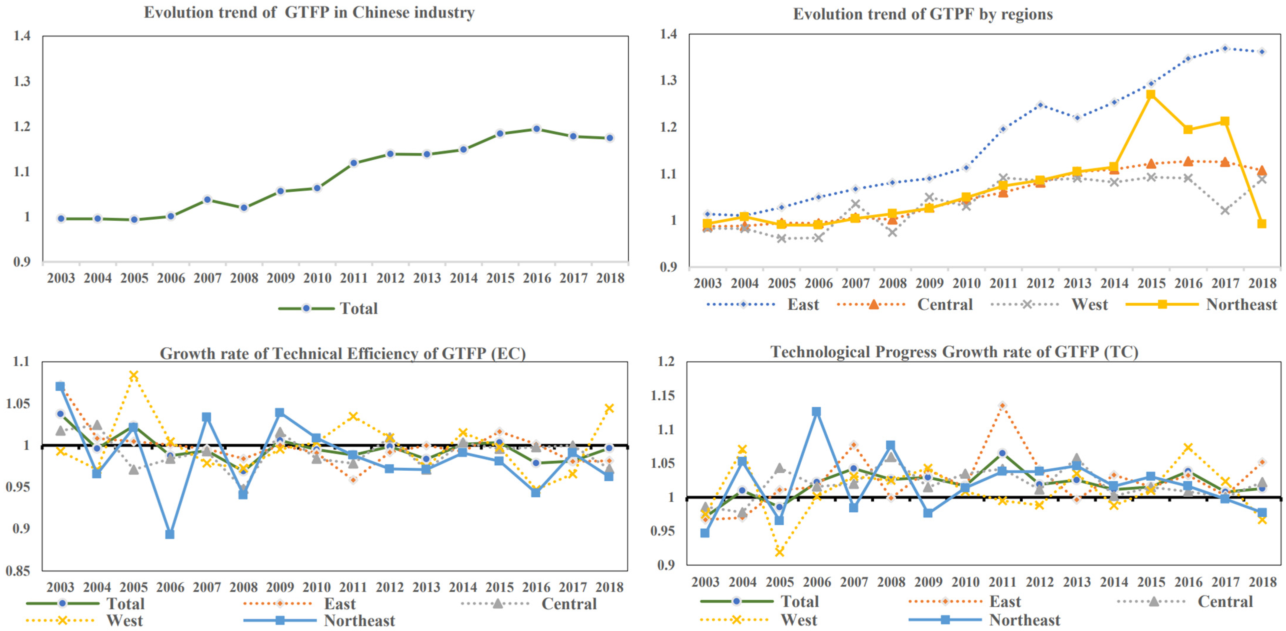
5.1. The Trend and Decomposition of GTFP in China’s Industrial Sectors
5.2. Analysis of Spatial Differences of China’s Industrial GTFP
5.2.1. Overall Differences
5.2.2. Intra-Regional Differences
5.2.3. Inter-Regional Differences
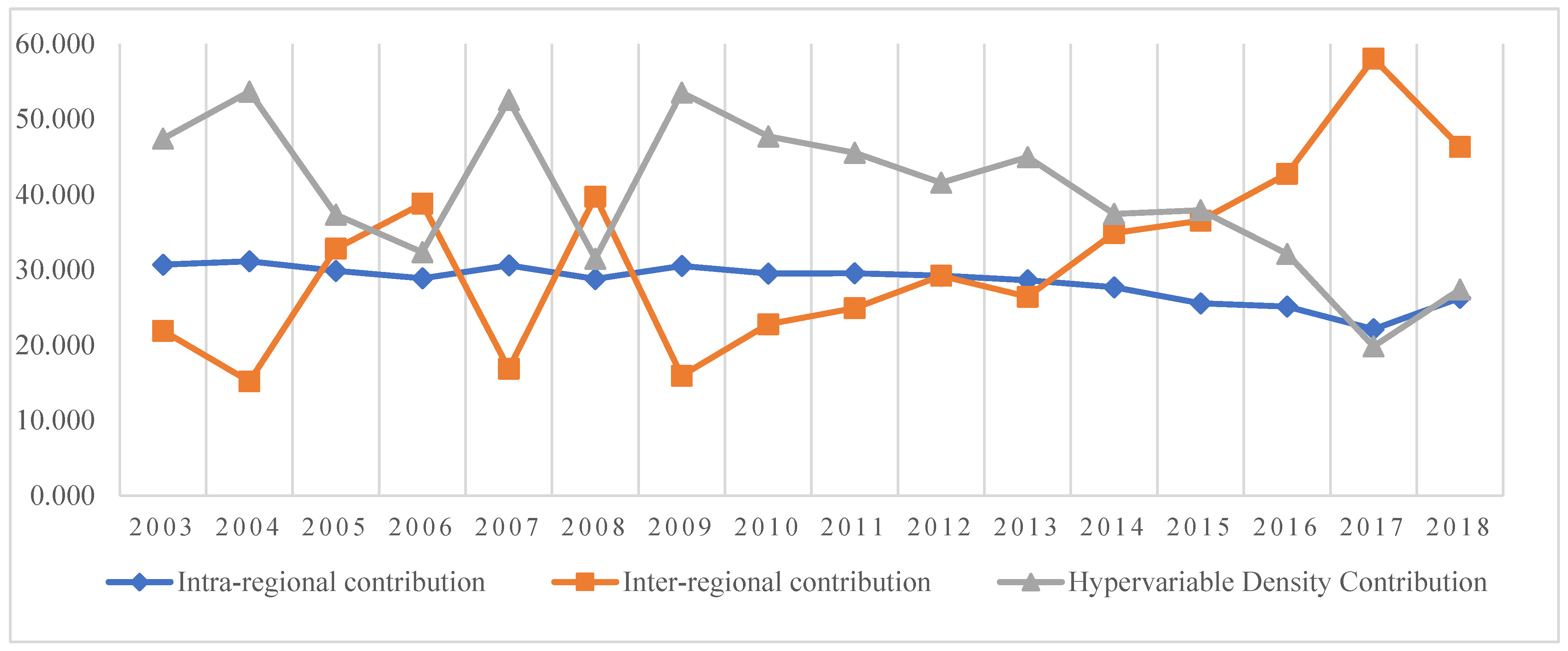
5.2.4. Sources of Differences
5.3. Spatial-Temporal Heterogeneity Analysis of Influencing Factors of GTFP in Chinese Industry
6. Conclusions and Policy Recommendations
6.1. Summary and Conclusions
- (1)
- From 2003 to 2018, China’s industrial GTFP exhibited an overall dynamic trend of “growth-steady growth-decline”. The growth rate of eastern China was much higher than that of other regions, and the GTFP of northeast and western China fluctuated widely after 2016. The decomposition analysis reveals that the technical efficiency of China’s industrial sector has lowered the GTFP, and technological progress is an essential source of promoting the growth of China’s industrial GTFP.
- (2)
- The western region has the greatest intra-regional differences in GTFP growth, followed by the eastern and northeast regions, and the central region has the smallest intra-regional differences. The primary source of the uneven distribution of GTFP in industry is inter-regional difference, with the average contribution rate to Gini coefficient at 71.617%. The regional difference in GTFP is gradually widening.
- (3)
- From the perspective of factor supply, technological innovation, government regulation, and external environment, there is significant spatial and temporal heterogeneity in the impact of different factors on industrial GTFP in China’s four regions. For the eastern, central, and western regions, (i) the input of science and technology and the level of urbanization have a long-term promoting effect on GTFP. (ii) The influence of FDI on GTFP has experienced an “N-type” fluctuation of first promoting, then inhibiting, and then promoting. (iii) Capital input, patent output, and technology import have a long-term negative impact on GTFP. (iv) Environmental governance and financial support have a “U-shaped” impact on the eastern, central, and western regions. In northeast China, (i) capital drive, energy structure, and marketization process exert a positive impact, (ii) while environmental governance and urbanization have a strong negative impact. (iii) Scientific and technological input has a U-shaped influence on GTFP, and (iv) financial support has the inverse U-shape effect.
6.2. Policy Recommendations
- (1)
- Promote coordinated development across regions and form an industrial layout connecting regions with complementary advantages and reasonable division of labor. Initiate a new round of urbanization to accelerate industrial transfer, to promote employment and infrastructure construction (such as transportation, logistics, medical services, and environmental protection), and to optimize urban spatial planning and promote the cross-regional flow of factors of production. In particular, more attention should be paid to mitigating the impact of population loss in northeast China.
- (2)
- Accelerate industrial transformation and structural upgrading, and through technological innovation, drive high-quality industrial development. In addition, increase the share of advanced manufacturing in industry and strengthen financial support for the real economy to ease the difficulty faced by industrial enterprises in obtaining loans. Meanwhile, promote sustained innovation by enterprises and encourage high-quality industrial development through boosting investment in scientific and technological innovation and taking measures to accelerate the application of scientific and technological achievements.
- (3)
- Diversify environmental regulation policies (again, considering regional heterogeneities) and vigorously promote cleaner production. As the marginal effect of environmental governance energy efficiency decreases in the eastern and central regions, the development mode needs to be changed by starting from the technology source and adopting the “three-pronged” management mode of energy saving, carbon reduction, and pollution control.
- (4)
- Promote industrial clustering and improve the efficiency of intensive land use. Industrial agglomeration without scale efficiency is a common problem in all major regions of China. The first step to address the problem of low FDI utilization efficiency in the central region is to establish an effective exchange platform so as to expedite local absorption of FDI advanced production technology. Second, promote effective agglomeration of upstream and downstream enterprises of the industrial chain, reduce logistics costs, further improve industrial production efficiency, and fully transform technological advantages into economic advantages.
Author Contributions
Funding
Institutional Review Board Statement
Informed Consent Statement
Data Availability Statement
Acknowledgments
Conflicts of Interest
References
- Rahman, M.M.; Kashem, M.A. Carbon emissions, energy consumption and industrial growth in Bangladesh: Empirical evidence from ARDL cointegration and Granger causality analysis. Energy Policy 2017, 110, 600–608. [Google Scholar] [CrossRef]
- Shahbaz, M.; Lean, H.H.; Shabbir, M.S. Environmental Kuznets Curve hypothesis in Pakistan: Cointegration and Granger causality. Renew. Sustain. Energy Rev. 2012, 16, 2947–2953. [Google Scholar] [CrossRef] [Green Version]
- Waheed, R.; Sarwar, S.; Wei, C. The survey of economic growth, energy consumption and carbon emission. Energy Rep. 2019, 5, 1103–1115. [Google Scholar] [CrossRef]
- Jiang, T.; Huang, S.; Yang, J. Structural carbon emissions from industry and energy systems in China: An input-output analysis. J. Clean. Prod. 2019, 240, 118116. [Google Scholar] [CrossRef]
- Li, K.; Lin, B. Impact of energy conservation policies on the green productivity in China’s manufacturing sector: Evidence from a three-stage DEA model. Appl. Energy 2016, 168, 351–363. [Google Scholar] [CrossRef]
- Yang, Z.; Fan, M.; Shao, S.; Yang, L. Does carbon intensity constraint policy improve industrial green production performance in China? A quasi-DID analysis. Energy Econ. 2017, 68, 271–282. [Google Scholar] [CrossRef]
- Cheng, M.; Shao, Z.; Gao, F.; Yang, C.; Tong, C.; Yang, J.; Zhang, W. The effect of research and development on the energy conservation potential of China’s manufacturing industry: The case of east region. J. Clean. Prod. 2020, 258, 120558. [Google Scholar] [CrossRef]
- Wang, Q.; Zhao, C. Regional difference and driving factors of industrial carbon emissions performance in China. Alex. Eng. J. 2021, 60, 301–309. [Google Scholar] [CrossRef]
- Fu, S.; Ma, Z.; Ni, B.; Peng, J.; Zhang, L.; Fu, Q. Research on the spatial differences of pollution-intensive industry transfer under the environmental regulation in China. Ecol. Indic. 2021, 129, 107921. [Google Scholar] [CrossRef]
- Yalçınkaya, Ö.; Hüseyni, İ.; Çelik, A.K. The Impact of Total Factor Productivity on Economic Growth for Developed and Emerging Countries: A Second-generation Panel Data Analysis. Margin J. Appl. Econ. Res. 2017, 11, 404–417. [Google Scholar] [CrossRef]
- Chen, S.Y. Green industrial revolution in China: A perspective from the change of environmental total factor productivity. Econ. Res. J. 2010, 45, 21–34. [Google Scholar]
- Chen, S.; Golley, J. ‘Green’ productivity growth in China’s industrial economy. Energy Econ. 2014, 44, 89–98. [Google Scholar] [CrossRef]
- Zhang, J.; Tan, W. Study on the green total factor productivity in main cities of China. Zb. Rad. Ekon. Fak. Rijeci Časopis Ekon. Teor. Praksu 2016, 34, 215–234. [Google Scholar]
- Wang, K.; Wei, Y.-M. Sources of energy productivity change in China during 1997–2012: A decomposition analysis based on the Luenberger productivity indicator. Energy Econ. 2016, 54, 50–59. [Google Scholar] [CrossRef]
- Xia, F.; Xu, J. Green total factor productivity: A re-examination of quality of growth for provinces in China. China Econ. Rev. 2020, 62, 101454. [Google Scholar] [CrossRef]
- Yin, J.-Y.; Cao, Y.-F.; Tang, B.-J. Fairness of China’s provincial energy environment efficiency evaluation: Empirical analysis using a three-stage data envelopment analysis model. Nat. Hazards 2019, 95, 343–362. [Google Scholar] [CrossRef]
- Wang, C. Decomposing energy productivity change: A distance function approach. Energy 2007, 32, 1326–1333. [Google Scholar] [CrossRef]
- Wang, Z.; Feng, C. Sources of production inefficiency and productivity growth in China: A global data envelopment analysis. Energy Econ. 2015, 49, 380–389. [Google Scholar] [CrossRef]
- Yang, L.; Ouyang, H.; Fang, K.; Ye, L.; Zhang, J. Evaluation of regional environmental efficiencies in China based on super-efficiency-DEA. Ecol. Indic. 2015, 51, 13–19. [Google Scholar]
- Wang, F.; Li, R.; Yu, C.; Xiong, L.; Chang, Y. Temporal-Spatial Evolution and Driving Factors of the Green Total Factor Productivity of China’s Central Plains Urban Agglomeration. Front. Environ. Sci. 2021, 9, 193. [Google Scholar] [CrossRef]
- Chung, Y.H.; Färe, R.; Grosskopf, S. Productivity and Undesirable Outputs: A Directional Distance Function Approach. J. Environ. Manag. 1997, 51, 229–240. [Google Scholar] [CrossRef] [Green Version]
- Oh, D.-H.; Heshmati, A. A sequential Malmquist–Luenberger productivity index: Environmentally sensitive productivity growth considering the progressive nature of technology. Energy Econ. 2010, 32, 1345–1355. [Google Scholar]
- Oh, D.-h. A global Malmquist-Luenberger productivity index. J. Product. Anal. 2010, 34, 183–197. [Google Scholar] [CrossRef]
- Liu, G.; Wang, B.; Zhang, N. A coin has two sides: Which one is driving China’s green TFP growth? Econ. Syst. 2016, 40, 481–498. [Google Scholar]
- Hu, J.-L.; Sheu, H.-J.; Lo, S.-F. Under the shadow of Asian Brown Clouds: Unbalanced regional productivities in China and environmental concerns. Int. J. Sustain. Dev. World Ecol. 2009, 12, 429–442. [Google Scholar] [CrossRef]
- Dan, S. Regional Differences in China’s Energy Efficiency and Conservation Potentials. China World Econ. 2007, 15, 96–115. [Google Scholar]
- Du, J.L.; Liu, Y.; Diao, W.X. Assessing Regional Differences in Green Innovation Efficiency of Industrial Enterprises in China. Int. J. Environ. Res. Public Health 2019, 16, 940. [Google Scholar]
- Chen, Y.; Yin, G.; Liu, K. Regional differences in the industrial water use efficiency of China: The spatial spillover effect and relevant factors. Resour. Conserv. Recycl. 2021, 167, 105239. [Google Scholar]
- Wang, D.T.; Gu, F.F.; Tse, D.K.; Yim, C.K. When does FDI matter? The roles of local institutions and ethnic origins of FDI. Int. Bus. Rev. 2013, 22, 450–465. [Google Scholar]
- Xu, B.; Lin, B.Q. Regional differences in the CO2 emissions of China’s iron and steel industry: Regional heterogeneity. Energy Policy 2016, 88, 422–434. [Google Scholar]
- Yan, Z.; Zou, B.; Du, K.; Li, K. Do renewable energy technology innovations promote China’s green productivity growth? Fresh evidence from partially linear functional-coefficient models. Energy Econ. 2020, 90, 104842. [Google Scholar] [CrossRef]
- Gao, Y.; Zhang, M.; Zheng, J. Accounting and determinants analysis of China’s provincial total factor productivity considering carbon emissions. China Econ. Rev. 2021, 65, 101576. [Google Scholar] [CrossRef]
- Wei, W.; Zhang, W.-L.; Wen, J.; Wang, J.-S. TFP growth in Chinese cities: The role of factor-intensity and industrial agglomeration. Econ. Model. 2020, 91, 534–549. [Google Scholar] [CrossRef]
- Fotheringham, A.S.; Crespo, R.; Yao, J. Geographical and Temporal Weighted Regression (GTWR). Geogr. Anal. 2015, 47, 431–452. [Google Scholar] [CrossRef] [Green Version]
- Tao, F.; Zhang, H.; Hu, J.; Xia, X.H. Dynamics of green productivity growth for major Chinese urban agglomerations. Appl. Energy 2017, 196, 170–179. [Google Scholar] [CrossRef]
- Fare, R.; Grosskopf, S.; Pasurkajr, C. Environmental production functions and environmental directional distance functions. Energy 2007, 32, 1055–1066. [Google Scholar] [CrossRef]
- Lin, B.; Chen, Z. Does factor market distortion inhibit the green total factor productivity in China? J. Clean. Prod. 2018, 197, 25–33. [Google Scholar] [CrossRef]
- Dagum, C. A new approach to the decomposition of the Gini income inequality ratio. Empir. Econ. 1997, 22, 515–531. [Google Scholar] [CrossRef]
- Huang, B.; Zhang, L.; Wu, B. Spatiotemporal analysis of rural-urban land conversion. Int. J. Geogr. Inf. Sci. 2009, 23, 379–398. [Google Scholar] [CrossRef]
- Shao, S.; Yang, L.; Yu, M.; Yu, M. Estimation, characteristics, and determinants of energy-related industrial CO2 emissions in Shanghai (China), 1994–2009. Energy Policy 2011, 39, 6476–6494. [Google Scholar] [CrossRef]
- Fan, M.; Shao, S.; Yang, L. Combining global Malmquist–Luenberger index and generalized method of moments to investigate industrial total factor CO2 emission performance: A case of Shanghai (China). Energy Policy 2015, 79, 189–201. [Google Scholar] [CrossRef]
- Wang, K.L.; Pang, S.Q.; Ding, L.L.; Miao, Z. Combining the biennial Malmquist-Luenberger index and panel quantile regression to analyze the green total factor productivity of the industrial sector in China. Sci. Total Environ. 2020, 739, 140280. [Google Scholar] [CrossRef]
- Ren, Y. Research on the green total factor productivity and its influencing factors based on system GMM model. J. Ambient. Intell. Humaniz. Comput. 2019, 11, 3497–3508. [Google Scholar] [CrossRef]
- Wang, K.; Wei, Y.-M. China’s regional industrial energy efficiency and carbon emissions abatement costs. Appl. Energy 2014, 130, 617–631. [Google Scholar] [CrossRef]
- Ma, X.; Zhang, J.; Ding, C.; Wang, Y. A geographically and temporally weighted regression model to explore the spatiotemporal influence of built environment on transit ridership. Comput. Environ. Urban Syst. 2018, 70, 113–124. [Google Scholar] [CrossRef]
- Yuan, H.; Feng, Y.; Lee, J.; Liu, H. The Spatio-Temporal Heterogeneity of Financial Agglomeration on Green Development in China Cities Using GTWR Model. Sustainability 2020, 12, 6660. [Google Scholar] [CrossRef]


| First Level Indicators | Second Level Indicators | Variable | Measuring Method |
|---|---|---|---|
| Factor supply | Capital input | Fx | Ratio of new fixed capital input of industrial enterprises to GDP |
| Energy structure | Energy | Ratio of coal consumption to energy consumption | |
| Technological progress | R&D investment | Tec | Ratio of R&D internal expenditure to GDP |
| Patent applications | Prop | Logarithm of patent applications of industrial enterprises above designated size with one year lag | |
| Technical modification | Imp | Ratio of total expenditure of industrial enterprises above designated size in technology introduction, adaptation, and absorption to GDP | |
| Structural factors | Environmental governance | Eno | Ratio of investment in local industrial pollution control to GDP |
| Industrial clustering | Indus | Location quotient | |
| Urbanization level | Urban | Urbanization rate | |
| Market environment | Degree of marketization | Market | Marketization index |
| Financial development | Fina | Ratio of outstanding loans of financial institutions to GDP | |
| Foreign direct investment | FDI | Ratio of total foreign investment to GDP |
| VarName | Obs | Mean | SD | Min | Median | Max |
|---|---|---|---|---|---|---|
| Capital stock | 510 | 7369.4588 | 6478.345 | 290.09 | 5676.46 | 35,890.02 |
| Labor input | 510 | 278.7029 | 304.838 | 10.42 | 169.04 | 1568.00 |
| Energy consumption | 510 | 7029.6566 | 5035.299 | 186.92 | 6104.01 | 26,726.53 |
| Expected output | 510 | 4890.9367 | 5509.606 | 83.78 | 3102.05 | 34,421.81 |
| So2 | 510 | 65.6223 | 44.129 | 1.06 | 55.64 | 200.30 |
| Co2 | 510 | 258.3891 | 185.188 | 14.00 | 205.80 | 912.20 |
| Gtfp | 480 | 1.0894 | 0.2098 | 0.5607 | 1.0440 | 1.8312 |
| Fx | 480 | 0.5049 | 0.1845 | 0.2253 | 0.4657 | 1.3264 |
| Energy | 480 | 0.9567 | 0.3906 | 0.0380 | 0.8959 | 2.4229 |
| Tec | 480 | 0.0139 | 0.0106 | 0.0017 | 0.0109 | 0.0617 |
| Prop | 480 | 7.3130 | 1.9707 | 1.9459 | 7.3019 | 12.5750 |
| Imp | 480 | 0.9925 | 0.8460 | 0.0664 | 0.7167 | 5.7127 |
| Eno | 480 | 0.0016 | 0.0013 | 0.0001 | 0.0013 | 0.0099 |
| Indus | 480 | 0.0134 | 0.0235 | 0.0000 | 0.0043 | 0.1322 |
| Urban | 480 | 0.5238 | 0.1441 | 0.2566 | 0.5050 | 0.8960 |
| Market | 480 | 6.4613 | 1.8996 | 2.3300 | 6.2700 | 11.7100 |
| Fina | 480 | 1.1943 | 0.4156 | 0.5372 | 1.1183 | 2.5847 |
| FDI | 480 | 0.0583 | 0.0695 | 0.0066 | 0.0307 | 0.7503 |
| Year | Total | East | Central | West | Northeast |
|---|---|---|---|---|---|
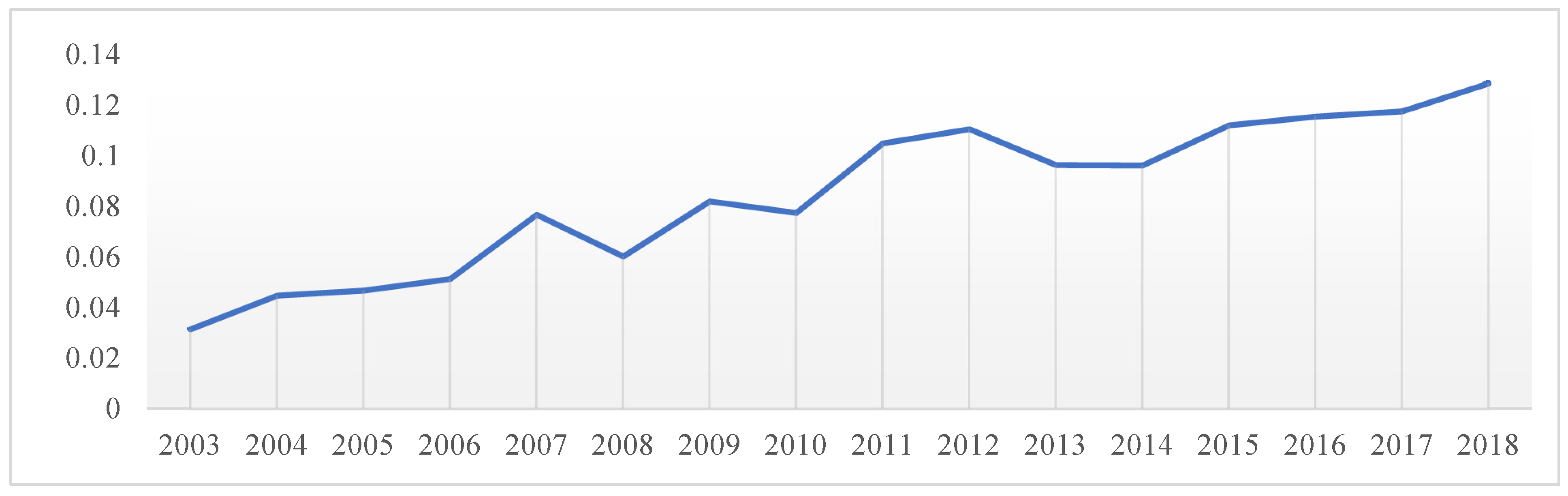
| 2003 | 0.0314 | 0.0112 | 0.0137 | 0.0580 | 0.0116 |
| 2004 | 0.0447 | 0.0160 | 0.0189 | 0.0851 | 0.0073 |
| 2005 | 0.0467 | 0.0325 | 0.0379 | 0.0659 | 0.0114 |
| 2006 | 0.0512 | 0.0371 | 0.0358 | 0.0686 | 0.0170 |
| 2007 | 0.0767 | 0.0428 | 0.0353 | 0.1263 | 0.0253 |
| 2008 | 0.0601 | 0.0515 | 0.0243 | 0.0777 | 0.0308 |
| 2009 | 0.0819 | 0.0499 | 0.0295 | 0.1330 | 0.0359 |
| 2010 | 0.0773 | 0.0558 | 0.0289 | 0.1134 | 0.0409 |
| 2011 | 0.1048 | 0.0823 | 0.0276 | 0.1502 | 0.0452 |
| 2012 | 0.1104 | 0.1007 | 0.0238 | 0.1446 | 0.0595 |
| 2013 | 0.0962 | 0.0696 | 0.0213 | 0.1380 | 0.0660 |
| 2014 | 0.0961 | 0.0755 | 0.0257 | 0.1242 | 0.0738 |
| 2015 | 0.1120 | 0.0813 | 0.0314 | 0.1289 | 0.1444 |
| 2016 | 0.1154 | 0.0874 | 0.0373 | 0.1239 | 0.1400 |
| 2017 | 0.1175 | 0.0958 | 0.0318 | 0.0924 | 0.1572 |
| 2018 | 0.1285 | 0.1061 | 0.0464 | 0.1438 | 0.0475 |
| Year | East-Central | East-West | East-Northeast | Central-West | Central-Northeast | West-Northeast |
|---|---|---|---|---|---|---|
| 2003 | 0.0165 | 0.0380 | 0.0145 | 0.0404 | 0.0135 | 0.0391 |
| 2004 | 0.0198 | 0.0579 | 0.0133 | 0.0579 | 0.0155 | 0.0551 |
| 2005 | 0.0387 | 0.0543 | 0.0312 | 0.0537 | 0.0289 | 0.0440 |
| 2006 | 0.0439 | 0.0618 | 0.0397 | 0.0547 | 0.0300 | 0.0494 |
| 2007 | 0.0485 | 0.0955 | 0.0464 | 0.0873 | 0.0330 | 0.0845 |
| 2008 | 0.0530 | 0.0759 | 0.0528 | 0.0548 | 0.0314 | 0.0595 |
| 2009 | 0.0488 | 0.1027 | 0.0521 | 0.0919 | 0.0354 | 0.0952 |
| 2010 | 0.0558 | 0.0959 | 0.0580 | 0.0812 | 0.0380 | 0.0872 |
| 2011 | 0.0820 | 0.1315 | 0.0840 | 0.1032 | 0.0433 | 0.1133 |
| 2012 | 0.0924 | 0.1394 | 0.1011 | 0.0981 | 0.0526 | 0.1149 |
| 2013 | 0.0702 | 0.1220 | 0.0822 | 0.0931 | 0.0558 | 0.1119 |
| 2014 | 0.0784 | 0.1231 | 0.0911 | 0.0848 | 0.0628 | 0.1077 |
| 2015 | 0.0874 | 0.1343 | 0.1328 | 0.0903 | 0.1230 | 0.1558 |
| 2016 | 0.1018 | 0.1398 | 0.1419 | 0.0893 | 0.1237 | 0.1479 |
| 2017 | 0.1092 | 0.1543 | 0.1573 | 0.0727 | 0.1390 | 0.1587 |
| 2018 | 0.1282 | 0.1632 | 0.1672 | 0.1040 | 0.0646 | 0.1127 |
| Year | Intraregional Contribution Rate | Interregional Net Difference Contribution | Hypervariable Density Contribution Rate |
|---|---|---|---|
| 2003 | 30.685 | 21.896 | 47.419 |
| 2004 | 31.150 | 15.181 | 53.669 |
| 2005 | 29.869 | 32.801 | 37.330 |
| 2006 | 28.870 | 38.785 | 32.346 |
| 2007 | 30.600 | 16.848 | 52.552 |
| 2008 | 28.788 | 39.733 | 31.479 |
| 2009 | 30.514 | 15.941 | 53.545 |
| 2010 | 29.506 | 22.776 | 47.717 |
| 2011 | 29.545 | 24.907 | 45.548 |
| 2012 | 29.226 | 29.208 | 41.566 |
| 2013 | 28.616 | 26.420 | 44.964 |
| 2014 | 27.682 | 34.889 | 37.430 |
| 2015 | 25.553 | 36.529 | 37.919 |
| 2016 | 25.122 | 42.750 | 32.128 |
| 2017 | 22.118 | 58.053 | 19.829 |
| 2018 | 26.285 | 46.314 | 27.401 |
| Variable | Urban | Market | Tec | Prop | Fina | Fx |
| VIF | 4.911 | 4.092 | 3.309 | 3.279 | 2.382 | 2.131 |
| 1/VIF | 0.204 | 0.244 | 0.302 | 0.305 | 0.42 | 0.469 |
| Variable | Imp | FDI | Energy | Indus | Eno | Mean |
| VIF | 1.93 | 1.919 | 1.832 | 1.761 | 1.693 | 2.658 |
| 1/VIF | 0.518 | 0.521 | 0.546 | 0.568 | 0.591 | / |
| Variable | 2 × SE (OLS) | Interquartile (GTWR) |
| Fx | −0.1250 | −0.4876 |
| Energy | −0.0548 | −0.2328 |
| Tec | −2.7208 | −12.1396 |
| Prop | −0.0146 | −0.0513 |
| Imp | −0.0260 | −0.0873 |
| Eno | −15.3872 | −27.1309 |
| Indus | −0.8944 | −1.9918 |
| Urban | −0.2432 | −0.8639 |
| Market | −0.0168 | −0.0214 |
| Fina | −0.0588 | −0.1220 |
| FDI | −0.3152 | −0.7140 |
| Variable | TWR | GWR | GTWR | ||||||
| First Quartile | Median | Third Quartile | First Quartile | Median | Third Quartile | First Quartile | Median | Third Quartile | |
| Fx | −0.263 | −0.195 | −0.069 | −0.766 | −0.463 | −0.116 | −0.554 | −0.318 | −0.066 |
| Energy | 0.004 | 0.015 | 0.022 | −0.212 | −0.056 | 0.048 | −0.169 | −0.011 | 0.064 |
| Tec | −2.258 | −0.166 | 0.773 | −1.877 | 0.914 | 12.581 | −1.371 | 1.729 | 10.768 |
| Prop | −0.063 | −0.030 | −0.019 | −0.029 | 0.004 | 0.029 | −0.048 | −0.020 | 0.003 |
| Imp | −0.211 | −0.096 | −0.033 | −0.033 | −0.021 | −0.003 | −0.100 | −0.041 | −0.013 |
| Eno | −0.581 | 14.636 | 19.365 | −10.017 | 7.291 | 17.088 | −13.269 | 0.316 | 13.862 |
| Indus | 0.063 | 0.204 | 1.078 | −1.881 | −1.207 | 0.211 | −1.877 | −0.857 | 0.115 |
| Urban | 0.656 | 0.993 | 1.164 | 0.370 | 0.637 | 1.175 | 0.338 | 0.681 | 1.202 |
| Market | −0.009 | −0.004 | −0.001 | −0.018 | −0.005 | 0.006 | −0.011 | −0.002 | 0.010 |
| Fina | −0.078 | −0.045 | −0.002 | −0.045 | −0.001 | 0.066 | −0.106 | −0.044 | 0.016 |
| FDI | −0.201 | −0.070 | 0.225 | −0.409 | −0.221 | 0.087 | −0.428 | −0.117 | 0.286 |
| Variable | Globe-OLS | TWR | GWR | GTWR |
| R2 | 0.3353 | 0.5142 | 0.8025 | 0.9009 |
| Adj. R2 | / | 0.5023 | 0.7979 | 0.8985 |
| RSS | 14.013 | 10.263 | 4.1723 | 2.0942 |
| AICc | / | −412.183 | −715.875 | −862.824 |
| Bandwidth | / | 0.2357 | 0.1150 | 0.1150 |
Publisher’s Note: MDPI stays neutral with regard to jurisdictional claims in published maps and institutional affiliations. |
© 2022 by the authors. Licensee MDPI, Basel, Switzerland. This article is an open access article distributed under the terms and conditions of the Creative Commons Attribution (CC BY) license (https://creativecommons.org/licenses/by/4.0/).
Share and Cite
Xiao, S.; Wang, S.; Zeng, F.; Huang, W.-C. Spatial Differences and Influencing Factors of Industrial Green Total Factor Productivity in Chinese Industries. Sustainability 2022, 14, 9229. https://doi.org/10.3390/su14159229
Xiao S, Wang S, Zeng F, Huang W-C. Spatial Differences and Influencing Factors of Industrial Green Total Factor Productivity in Chinese Industries. Sustainability. 2022; 14(15):9229. https://doi.org/10.3390/su14159229
Chicago/Turabian StyleXiao, Suyang, Susu Wang, Fanhua Zeng, and Wei-Chiao Huang. 2022. "Spatial Differences and Influencing Factors of Industrial Green Total Factor Productivity in Chinese Industries" Sustainability 14, no. 15: 9229. https://doi.org/10.3390/su14159229
APA StyleXiao, S., Wang, S., Zeng, F., & Huang, W.-C. (2022). Spatial Differences and Influencing Factors of Industrial Green Total Factor Productivity in Chinese Industries. Sustainability, 14(15), 9229. https://doi.org/10.3390/su14159229