Abstract
Regional flood frequency analysis (RFFA) is a powerful method for interrogating hydrological series since it combines observational time series from several sites within a region to estimate risk-relevant statistical parameters with higher accuracy than from single-site series. Since RFFA extreme value estimates depend on the shape of the selected distribution of the data-generating stochastic process, there is need for a suitable goodness-of-distributional-fit measure in order to optimally utilize given data. Here we present a novel, least-squares-based measure to select the optimal fit from a set of five distributions, namely Generalized Extreme Value (GEV), Generalized Logistic, Gumbel, Log-Normal Type III and Log-Pearson Type III. The fit metric is applied to annual maximum discharge series from six hydrological stations along the Sava River in South-eastern Europe, spanning the years 1961 to 2020. Results reveal that (1) the Sava River basin can be assessed as hydrologically homogeneous and (2) the GEV distribution provides typically the best fit. We offer hydrological-meteorological insights into the differences among the six stations. For the period studied, almost all stations exhibit statistically insignificant trends, which renders the conclusions about flood risk as relevant for hydrological sciences and the design of regional flood protection infrastructure.
1. Introduction
Floods are among the most impactful natural disasters and can cause significant human casualties and economic damage [1,2]. In Europe, numerous large rivers have been affected by extreme flood events since the 1990s, causing billions of Euros in damages [3,4,5]. Such impacts are expected to increase in the future partly due to climate change, and partly due to exposure of larger populations and economic growth [6,7].
The following list of works on observed river floods during the past decades and centuries may help the reader to put the current analysis into a wider geographical context: [4,8,9,10,11,12,13,14,15,16,17,18,19,20]. These papers include analyses of meteorological and demographic causes of extreme river flooding effects and also provide additional costs estimates.
The State of the Global Climate 2020 report [21] (WMO, 2021) marked that year as exceptional for worldwide flooding and other hydro-meteorological extremes. Such major events are expected to become more common in the future due to the increase of water vapour in the atmosphere (i.e., the Clausius-Clapeyron equation) leading to more intense precipitation events and, as a consequence, to more floods [22,23,24,25]. This has been confirmed by high-resolution regional climate modelling for Europe [26,27]. Moreover, expansion of cities, construction of roads and bridges across rivers, can all affect floodplain hydraulics and thereby change flood risks for exposed populations and assets [4,28]. Thus, for flood risk management purposes it is important that periodic assessments of rivers are conducted, especially regarding long-term discharge patterns. This can be achieved via flood frequency analysis (FFA), which can offer important information regarding river hydrological behaviour, also in changing environment [29,30,31,32].
For the determination of flood magnitude with a given return period, the most commonly applied statistical data-based approach is FFA. The standard method of FFA fits mathematical functions to available data and extrapolates the tails of the distribution to estimate the probability and magnitude of extreme events [33]. When sufficient data are available at a single gauging station, an extreme value distribution is typically fitted to the observed data, indicating an at-site FFA or local model [34]. However, for stations with incomplete or short data series, as well as for ungauged sites, data from comparably situated or nearby gauging stations can be used. This approach is known as regional flood frequency analysis (RFFA) [34]. Reliable estimates of magnitude and frequency of floods are essential for the design of different hydraulic structures such as spillways, levees, bridges, dams, irrigation ditches, bridges and urban drainage systems [35].
In recent years, many at-site FFA of different hydrological variables have been conducted for Europe and other parts of the world [22,29,35,36,37].
However, there is growing interest in the use of RFFA across Europe as evidenced by research in Germany [38], Norway [39], Poland [40], the Pannonian basin [31], the Tisza River basin [41] and the Danube River basin [42]. This is because accuracy can be improved by drawing on the information content of multiple sites [43]. Moreover, RFFA techniques offer opportunities for further development and application in decision-making [35,44].
Floods in Serbia are mostly caused by either (1) flow of humid air masses originating from the Atlantic Ocean, or (2) rapid snow melt from the Dinaric mountains associated with föhn winds in early spring. In addition, we note that the formation of floods in further downstream parts of the study area is influenced by erosion processes and the presence of a dense river network (note that the average river length per area in Serbia is 747 m/km2), see for example [28]. In the spring of 2014, Croatia, Bosnia and Herzegovina, and Serbia, were impacted by a flood event unparalleled in the hydrological records of the region [45,46]. The major cause of this flood was a Vb-type cyclonic weather system [5] that remained stationary over South-eastern Europe for several days causing rainfall accumulations of up to 300 mm in three days [45,47]. In Serbia alone, these floods affected the territories of 24 municipalities and caused EUR 1.525 billion in damages [48]. Before the 2014 event, there were other widespread floods such as in 1933, 1937, 1940, 1947, 1964, 1974 and 2007 [49]. The most remarkable of these occurred in 1974, when historical record water levels and discharges were exceeded at all stations downstream of the Drina River confluence. These extremes were exceeded by the 2014 flood event.
Given that extreme floods in the Sava River are expected to occur more frequently with climate change, reliable FFA is essential for engineering practice. Accordingly, this paper concentrates on the estimation of extreme river discharges as follows. First, the research area is described with emphasis on the Sava River basin (Section 2). Next, we present the data (Section 3) and methods (Section 4) applied. In the discussion (Section 5), we compare our results with those obtained in similar studies. In particular, we address the following questions. (1) What is the appropriate regional frequency distribution for selected gauging stations along the Sava River? (2) Which frequency distribution should be used for RFFA for ungauged rivers within the Sava River basin? This paper is, to the best of our knowledge, the first RFFA for the Sava River basin. Hence, we also address the question (3) after the study’s novelty and limitations and the practical consequences that can be drawn for decision makers.
2. Research Area
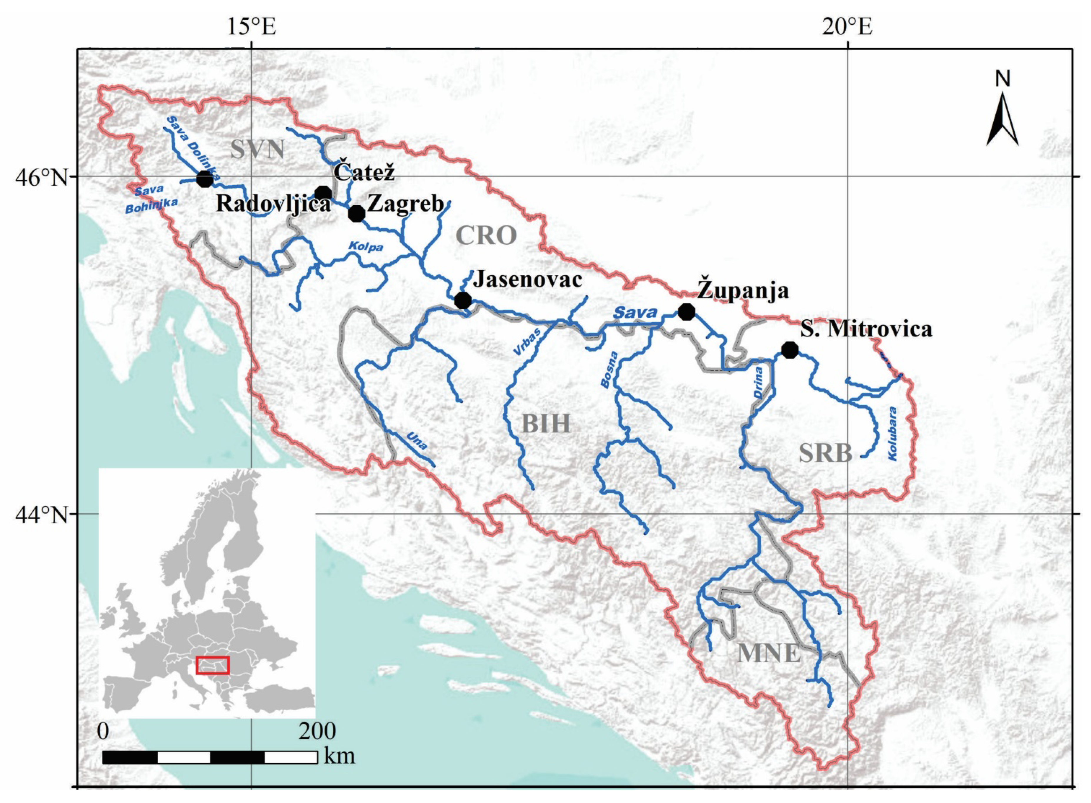
The Sava River basin, with a total area of around 97,000 km2, is the largest river catchment in South-eastern Europe and the second-largest sub-basin of the Danube River basin (Figure 1). It is shared by Slovenia, Croatia, Bosnia and Herzegovina, and Serbia; and a small part of 0.2% of the basin lies within Albania [50]. The Sava River originates in Slovenia, where two mountainous streams, Sava Dolinka and Sava Bohinjka, merge together near the town of Radovljica. The main tributaries of the Sava River are in downstream order the rivers Kolpa, Una, Vrbas, Bosna, Drina and Kolubara. Between the Una and the Drina, the majority of water comes from the south. Una, Vrbas, Bosna and Drina jointly contribute a discharge of 1149 m3/s to the Sava River, which is as much as 68% of the flow of the Sava at its confluence with the Danube [51]. Drina is the largest tributary with 371 m3/s or 22% of the flow of the Sava at its confluence with the Danube [51]. The length of the Sava River is 945 km to its confluence with the Danube River in Belgrade. Around 8 million people live in the Sava River basin [36].

Figure 1.
Sava River basin (red line), major rivers (blue lines), locations of the six selected gauging stations (black dots) and political borders with country names (grey) in ISO 3166-1 alpha-3 code. Inset is the position of study region within Europe.
The headwaters of the Sava River have a mountainous climate that transitions downstream to a temperate continental climate [52]. The temperate continental climate characterizes the right tributaries originating in the Dinaric mountains, whereas a moderate continental climate features on the left side of the basin, including the Pannonian plain [50]. The average annual precipitation in the Slovenian part of the Sava River ranges from 2210 mm representing the basin area of the Radovljica gauging station [32] to 1570 mm (Čatež gauging station)[53]. Over the Croatian part of the basin, the average annual precipitation is 855 mm [51]. The highest monthly amount of rainfall is usually recorded during June (91 mm), and the lowest typically in February (42 mm). For the Serbian part of the basin (S. Mitrovica station), the average is 577 mm, with the highest mean in June (84 mm) and the lowest in February (38 mm) [36].
The two rivers Sava Dolinka and Sava Bohinjka (Radovljica station) in Slovenia have an Alpine nival-pluvial regime [54]. Towards the Čatež gauging station, the river regime changes to an Alpine pluvial-nival type [54]. Further downstream, the river regime changes into the Peripannonian pluvial-nival (Zagreb and Jasenovac) and Pannonian pluvial-nival types (Županja and S. Mitrovica) [55].
3. Data
We utilized a 60-year (1961 to 2020) data set of daily discharges for six stations located on the Sava River (Figure 1). This data set was collected from three different national water authorities within the investigated river basin (namely the Slovenian Environment Agency; Meteorological and Hydrological Service, Croatia; and Republic Hydrometeorological Service of Serbia) (Table 1).

Table 1.
Geographical characteristics for observed stations.
The assumption of independence of extreme flows [56,57] needed for statistical analysis was met using the annual maximum series (AMS) of river discharges. AMS is a data type that is most frequently used for FFA as it is the most intuitive example of the block maxima method of the extreme value theory [31,58]. In FFA, a block usually represents a year, and so the highest discharge value within each year is selected [39]. One of the advantages of the AMS method is that it is straightforward to derive the distribution of the AMS values. Descriptive summary statistics of the AMS data are shown in Table 2.

Table 2.
Descriptive statistics for the AMS data from the six gauging stations on the Sava River; STD, standard deviation.
4. Methods
We applied the RFFA method combined with L-moments estimation [43] to the AMS data from six gauging stations along the Sava River. The advantage of RFFA is that it can be applied for flood risk estimation in situations where for a specific site the recording period is too short for a reliable estimation (or even where data are not available). The advantage of the L-moments technique (as compared with maximum likelihood estimation) is that it yields robust parameter estimates for various candidate distributions. In a statistical sense, the robustness of a method means that it yields reliable results even if assumptions underlying an analysis (such as the distributional shape) are violated [59]. The homogeneity of a region can then be assessed on the basis of a comparison test of the L-moments parameter estimates for the different gauging stations, supported by a goodness-of-fit test and L-moments diagrams [60,61].
The principle assumptions employed for the RFFA are that the observed data have been generated by a stationary random process [62,63]. One of the advantages of the AMS data type is that it allows statistical science to derive the distributional shape of the AMS values. This distribution is called Generalized Extreme Value (GEV) distribution, which emerges as the limit form of the maximum of many independent and identically distributed random elements in a time block (such as one year), and this statistical work has been performed in the late 1920s [64,65]. Furthermore, the AMS method provides flood event data that can be considered as independent and the frequency distributions generally conform to theoretical distributions [66]. For recent methodological developments in RFFA and its applications, see, for example, contributions about Canada [67] or Australia [68].
There are several guidelines issued by national hydrological services related to the choice of the distribution used in FFA. In the United States, the Log-Pearson Type III (LPIII) distribution should be used for FFA according to the United States Water Resources Council [69]; in the United Kingdom, usage of the GEV or the Generalized Logistic (GLO) distributions is advised according to the Flood Estimation Handbook [70]; in Poland, usage of the Pearson Type III (PIII) distribution is recommended [71]; and in Australia, it is recommended to compare the LPIII, GEV and Generalized Pareto estimation results before selecting a distribution [72].
For the rivers within the Pannonian basin, previous studies indicate that the best-fitting regional distribution shape could be lognormal [31]. However, further research conducted at individual stations showed that other distributions should be considered. For example, for the Bogojevo station on the Danube River, the PIII distribution was presented as the best fit [42]. A similar study conducted for the basin of the Tisza River (a tributary of the Danube River) also found that the best-fitting distribution is PIII [41]. Regarding the Sava River, Morlot et al. [42] demonstrated that PIII distribution is the best-fitting distribution for the Orljava-Pleternica gauging station (Croatia) as well as for the S. Mitrovica gauging station (Serbia). These results for the Sava River were further confirmed [36]. So far, in the Sava River basin and in the countries that share this basin, there are no official guidelines for FFA. Here, we applied the five most commonly used distributions in this region, namely: GEV, GLO, Gumbel, Log-Normal Type III (LNIII) and LPIII. The Appendix A provides the cumulative distribution functions (CDFs) for these shapes.
4.1. L-Moments Estimation for RFFA
The L-moments method was used to estimate distribution parameters. L-moments are a linear combination of the ranked observations [73]. What distinguishes L-moments from “conventional” statistical moments is their ability to describe a wider range of distributions and that they are more robust to the presence of outliers and, hence, less susceptible to estimation bias [43]. The most commonly employed method to calculate the L-moments is via probability weighted moments (PWM) [35,63]:
where br represents the rth-order PWM, while FX(x) is the CDF of X. Further, i for i = 0, 1, 2, 3, represents the unbiased sample estimators of the first four PWM as described by Hosking and Wallis [43]:
In these equations, X(j) indicates the ranked AMS values, that is, X(n) is the largest and X(1) is the smallest value. Furthermore, the first four L-moments [43] are given as follows:
That means, the first four L-moments follow straightforwardly from the PWM sample estimates. Another advantage of the usage of the L-moments approach is that these moments provide directly interpretable values for the mean or location (λ1), scale (λ2), shape (λ3) and kurtosis (λ4) of the distribution functions, a fact that is particularly useful in RFFA. Lastly, the L-moments ratios are calculated as follows [43]:
For RFFA, the L-moments approach should be applied in four steps [43], comprising: (1) screening of data, (2) identifying homogeneous regions, (3) choosing a regional frequency distribution and (4) estimating the parameters of the frequency distribution.
When determining the regional distribution and homogeneity of a region, the L-moments ratio diagram [66] should be constructed. The close association between LCs and LCk has been shown for the most frequently used probability distributions [43]. If a region is homogeneous, then the locations tend to group together in the L-moments ratio diagram. Closeness of the sample versions of LCs and LCk to a theoretical line of distributions (in case of three-parameter distributions), or of the sample mean to the theoretical points (in case of two-parameter distributions), determines the best-fitting parameter distribution describing the data from multiple sites [35]. If in the L-moments ratio diagram a point is located near the curve that represents a candidate distribution, that distribution can be considered as an acceptable selection for the regional distribution. The distance between a point and curve can be considered as measure of the goodness-of-fit. It is important to highlight that this method is dependent on the homogeneity of the regional data [74].
For further confirmation and for determination of the regional distribution, a statistical test of spatial homogeneity of the selected region should be conducted [43]. This test is based on a comparison of (1) the between-site variation in sample-LCv and (2) the expected variation for a homogeneous region. This test is calculated as follows:
In these equations, N is the number of sites; ni is the record length at site i; τ(i), τ3(i), τ4(i) are the sample values of LCv, LCs and LCk at site i, respectively; and , , are the regional sample averages of LCv, LCs and LCk, respectively. For a region to be considered as homogeneous, the test statistic values, Vi, for i = 1, 2, 3, should all be less than unity. If 1 ≤ Vi < 2, then a region is possibly homogeneous and if Vi ≥ 2, then the region can be assumed as heterogeneous [31,73].
In order to test whether a particular distributional shape provides a good fit to data, and furthermore in order to compare the fit quality of various candidate distributions, we employed two test measures.
The first test measure is the conventionally employed Z-statistic [43]. It is based on the comparison of sample- and population-LCk values for the different distributions:
In this equation, the acronym DIST refers to a particular distribution, is the population-LCk value for a particular candidate distribution, is the regional sample average of the LCk values and 𝜎4 is the regional sample standard deviation of the LCk values [31]. The test is performed by means of a comparison with a quantile of the standard normal distribution. We adopted a significance level of 5%, this means, a candidate distribution is considered suitable if .
A second test measure is introduced here since this paper aims not only to find the optimal distributional shape for the data from the Sava River basin, but also to contribute data-analytical tools for hydrology. As with the Kolmogorov-Smirnov test [75,76], our metric employs the empirical CDF of the AMS values. More specifically, let n be the sample size; X(j), j = 1, …, n, be the size-sorted AMS values (as in Section 4.1); and the empirical CDF, Fn(x), be defined as the number of X(j) ≤ x divided by n; then Fn(x) is a step-like curve in dependence on X(j), which goes from 0 to 1 and makes steps of size 1/n at each X(j) value. The smaller the distance is between a certain theoretical candidate distribution, Ftheo(x), the better the fit. The distance can be measured by means of the differences,
While the Kolmogorov-Smirnov test utilizes max{w(j)}, we employed a least-squares criterion,
Our metric allows all data points to contribute to the distance measurement since we require here that a suitable theoretical distribution should supply a good fit over the full range of data values. The factor (n − p)−1 is used to correct for the number of employed parameters, p, of a theoretical distribution. (That means, it is “easier” to fit a distribution with many parameters to data than with few, and Ockham’s Razor [56] indicates to prefer descriptions with fewer parameters.)
4.2. Trend Estimation
To test the stationarity assumption for the RFFA analysis, we employed linear ordinary least-squares regression [56,63] to determine trends in the AMS data. Let denote the time series, where T(k) is time and X(k) is AMS. The linear model is given by
where a is the intercept parameter, b the slope parameter and (k) the noise component. The minimization of the least-squares sum,
can be straightforwardly achieved by setting the first derivatives of SSQ (with respect to a and b) equal to zero, which yields two linear equations (called normal equations) that can be easily solved for the parameter estimates of a and b [63]. To assess the significance of a trend, an uncertainty measure (standard error) for the slope parameter, b, is indispensable. This study employed moving block bootstrap resampling [63] to obtain slope standard errors that are reliable. Moreover, the tests on (k) can indicate the presence of (1) non-normal distributions or (2) autocorrelation. The validity of the bootstrap for obtaining reliable uncertainty measures in regression analysis has been shown by means of statistical simulation experiments with artificial time series [63].
5. Results and Discussion
5.1. Regional Flood Frequency Analysis
The principle assumptions employed for the RFFA and the fitting of candidate probability distributions are that the observed data have been generated by a stationary random process [62,63]. Therefore, the first step was the calculation of the basic statistics of the AMS data (mean, median, maximum, standard deviation, skewness and kurtosis) for the six gauging stations (Table 2). These basic statistics were then used to define the selected frequency distributions for deriving the probability of exceeding a certain discharge value [77].
Hosking and Wallis [43] highlighted that there are little gains in accuracy of quantile or return level estimates when using regions that contain a large number of stations (above, say, 20) and that it is preferable to have a region with fewer stations but longer at-site records. In this study we used the six stations on the Sava River, which mainly have 60 years of data (Table 2). The positive skewness values (Table 2) indicate that the AMS data for the stations show deviations from a normal shape (in the form of right-skewness), as is to be expected for a block maxima series [63]. This result also justifies usage of the bootstrap procedure for trend estimation (Section 4.2).
5.2. Trend Analysis
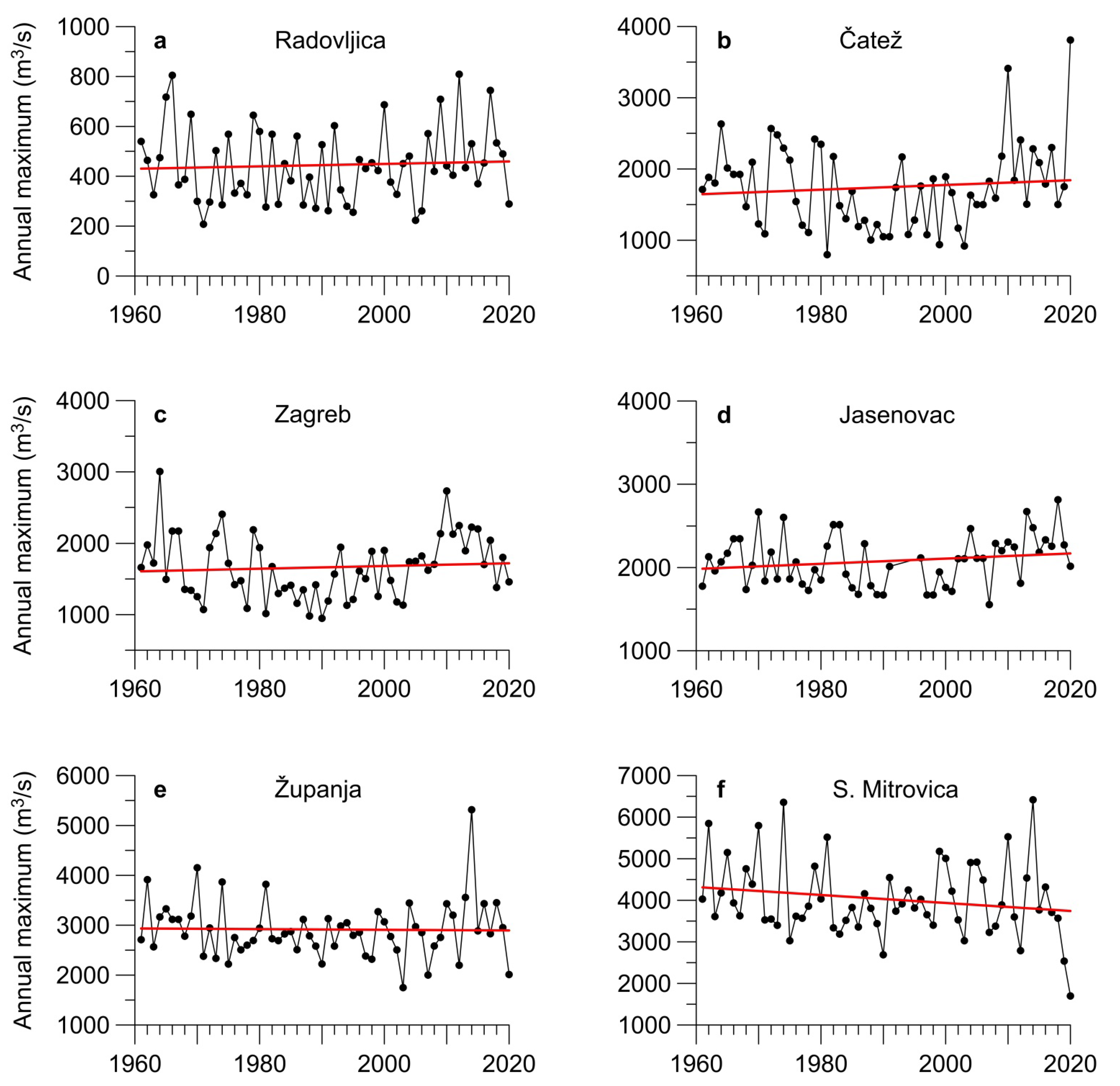
Linear trend analysis of the AMS at the six gauging stations along the Sava River showed mixed results (Figure 2, Table 3). AMS at the Radovljica and Čatež gauging stations in Slovenia demonstrate increasing but statistically insignificant trends (i.e., the absolute value of the slope estimate is less than its standard error). A statistically insignificant increase of AMS was also observed at the Zagreb gauging station during the study period.
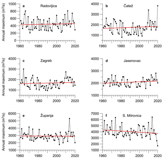

Table 3.
Slope estimates for the AMS data.
In general, negative AMS trends in the eastern part of the basin may be related to decreased snowmelt contributions from the Dinaric mountains, which represent the main water input for the right-hand tributaries. This influences the discharge regime of the Sava River downstream of Jasenovac [55]. Negative trends observed in AMS have also been attributed to (1) regional warming and (2) ocean–atmosphere modes of climate variability [2], the combination of which may further have caused a decline in precipitation and an increase in evaporation in the basin [22]. Comparable results of insignificantly decreasing river discharge trends were previously reported for the Danube and Sava Rivers [36,78].
At the two most downstream gauging stations (Županja and S. Mitrovica), maximum annual discharges are decreasing, likely as a consequence of a considerably larger catchment area for these stations and because large tributaries join the Sava River downstream. Consequently, the river discharge regime is more stable and maximum discharges are less influenced by severe and spatially limited precipitation. Presented results are consistent with other studies [22,79,80], which project decreasing discharge for major rivers in central and southern Europe. Furthermore, river modelling indicates a decreasing discharge of up to 40% for the Sava River at its lower course (S. Mitrovica station) [81].
5.3. Homogeneity Assessment and Regional Flood Frequency Analysis
The numerical results of the three homogeneity measures V1, V2 and V3 (Table 4) indicate that after Hosking and Wallis [43] we can consider the Sava River basin as acceptably homogeneous. Since all measures are less than unity, no further inspection of the data or of the cross-correlation between sites was necessary. That means, that the AMS data from the Sava River basin can be meaningfully applied for RFFA and also for a subsequent quantile estimation for gauged and ungauged rivers within the basin.

Table 4.
Homogeneity test of Sava River basin.
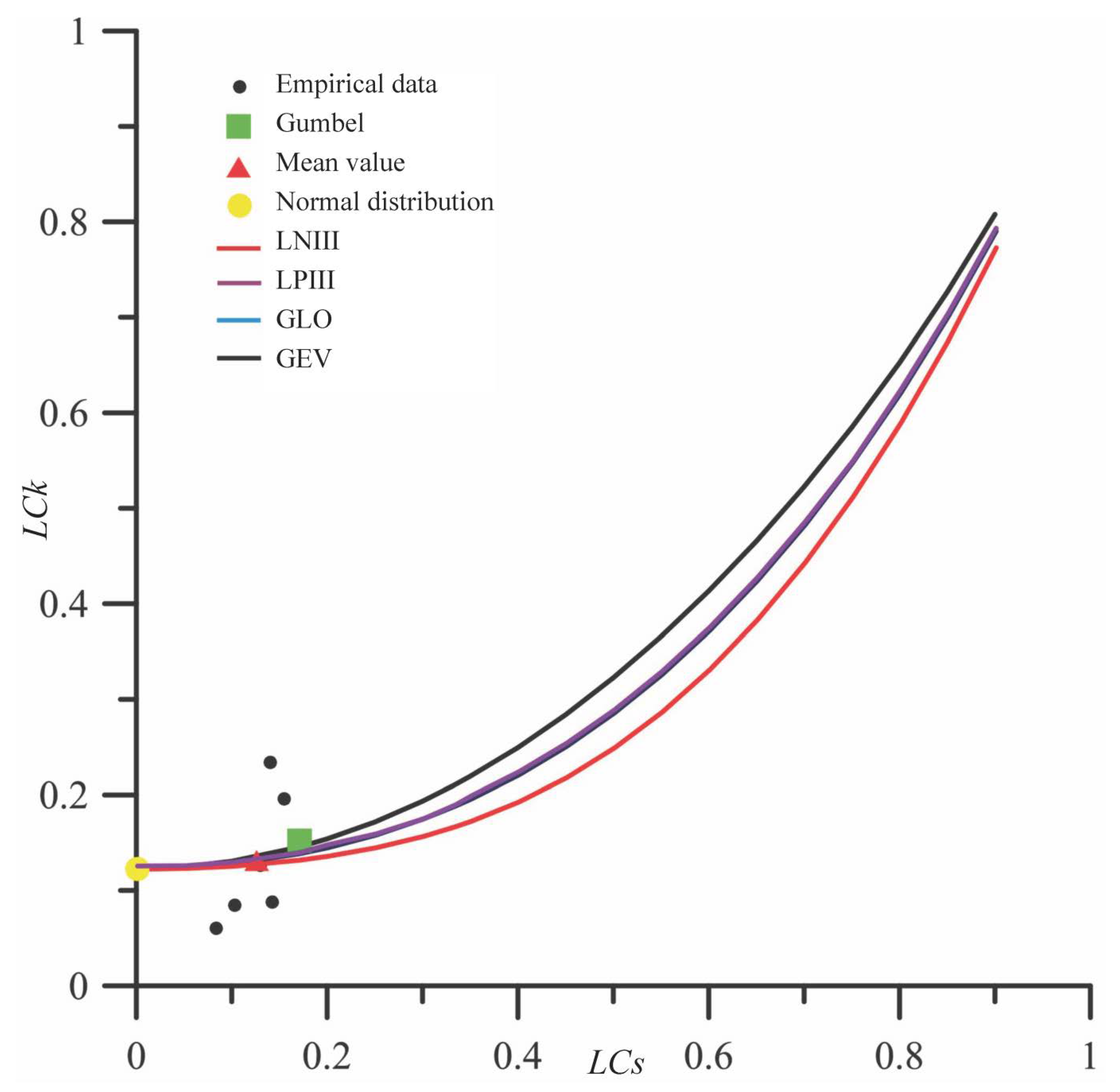
Since the basin homogeneity could be confirmed, the goodness-of-fit test and the L-moments diagram were used for the determination of the best-fitting distribution for RFFA (Figure 3).
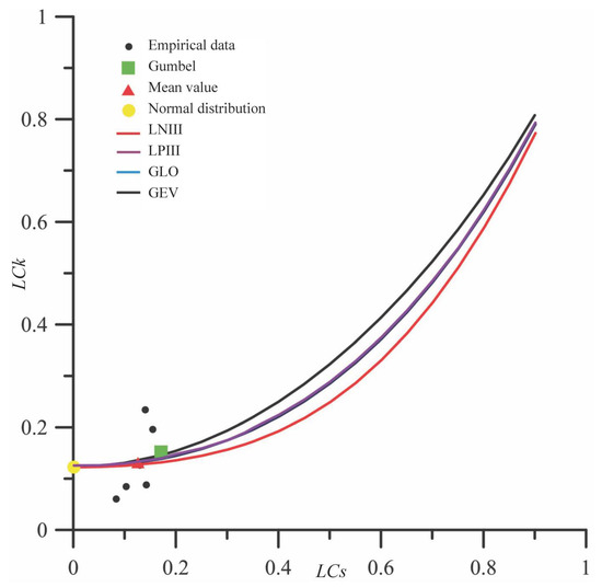
Figure 3.
L-moments ratio diagram for the six selected gauging stations (1961–2020) in the Sava River basin.
Owing to the robustness of the L-moments, station sample points can be expected to be randomly distributed above and below the theoretical line of an appropriate distribution. The results (Figure 3) show that there is no clear variation of LCk and LCs within the Sava River basin. Most data points display a tendency to group around the GEV and GLO distribution functions. In such cases, the mean value can be used as a reliable indicator of the best-fitting distribution [82]. Our results appear to indicate that the GEV distribution is the best-fitting distributional shape in the case of the Sava River basin.
For the purpose of identifying a common regional distribution that can be applied for ungauged rivers within the basin, the Z-statistic was calculated. The results reveal that all five distributions satisfy the test criterion namely GEV (Z = −0.06), GLO (Z = −0.20), Gumbel (Z = 0.28), LNIII (Z = 0.38) and LPIII (Z = 0.27). Since the absolute value of Z for the GEV distribution is the lowest, this is another indication that this distribution is valid for the Sava River basin as a whole. These findings are consistent with an FFA for Slovenia, where the GEV was identified as the best-fitting regional distribution [83]. Furthermore, results show that data from the gauging stations in the Sava River basin can be used for RFFA, and this application increases the reliability of the quantile estimates for both ungauged and gauged tributaries.
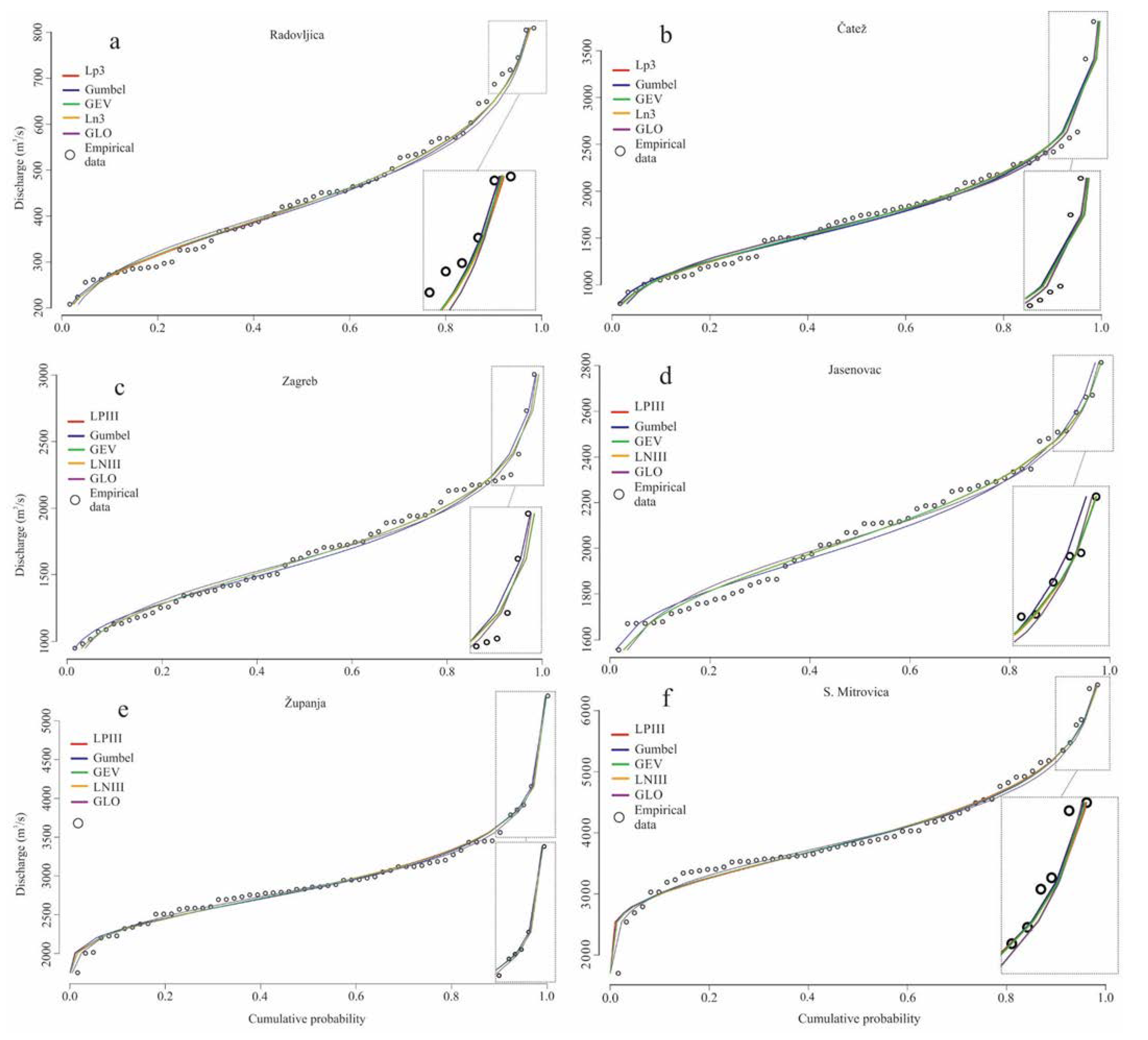
In order to examine the goodness-of-fit of the selected distribution to the empirical data, the CDFs were calculated for the analysed hydrological stations (Figure 4).
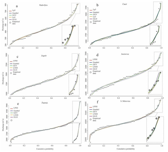
Figure 4.
FFA results: CDFs of empirical data and fitted candidate distributions for the six selected gauging stations in the Sava River basin ((a), Radovljica; (b), Čatež; (c), Zagreb; (d), Jasenovac; (e), Županja; (f), S. Mitrovica).
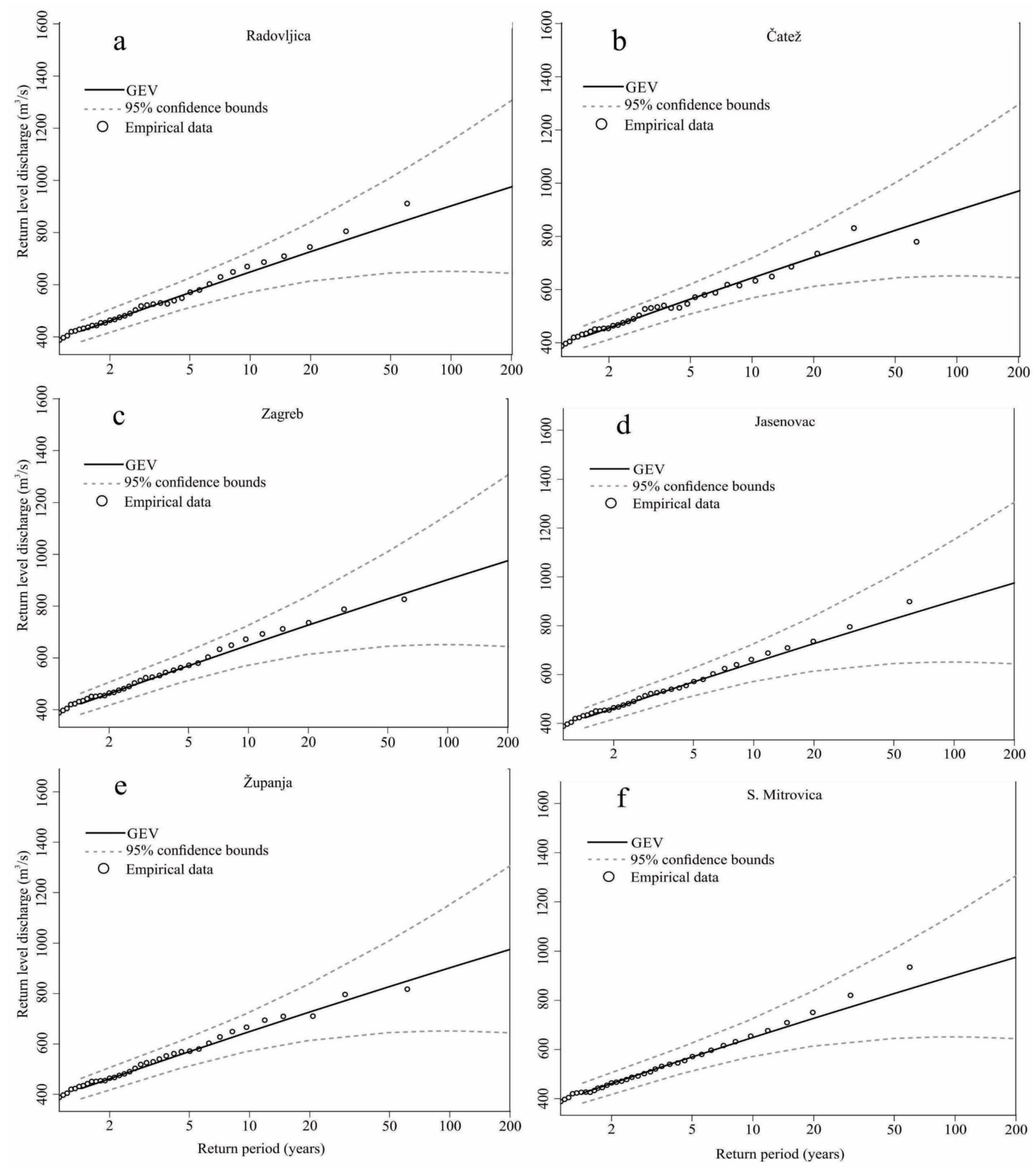
From Figure 4 it is notable that at the highest values (i.e., floods), several candidate distributions are in good agreement with the empirical data. However, the GEV distribution is in good agreement for the entire range of empirical data and therefore delivers the best goodness-of-fit measures (Table 5).

Table 5.
Results of goodness-of-distributional-fit measures u (Equation (18); dimensionless) of candidate distributions to observed station data.
Owing to the superiority of the distributional fit (Figure 4), the GEV is used to estimate the risk curves [63], that is, the return level in dependence on the return period (Figure 5). It is important to point out the inherent uncertainties (expressed as 95% confidence bounds) in the estimated return levels, which are due to the sampling variability, that is, a finite data set of noise-affected observations [31]. As expected, the range of uncertainty increases for longer return periods [29,31,56,63]. Despite the associated uncertainties of the estimated risk curves, the GEV distributions with their 95% confidence bounds can provide useful quantitative information for the construction of water infrastructure. For example, a precautionary guideline could be to apply the upper 95% confidence bound for a return period of 100 years. Mudelsee [63] recommends that the return period should be of the same order as the length of a series because the uncertainties increase with the return period (Figure 5). For the Sava River with record lengths of 60 years (Table 1), an upper bound estimate for a return period of 100 years may be suitable, whereas a bound of 500 years is certainly not.

Figure 5.
Estimated at-site return levels with 95% confidence bounds for GEV for the six selected gauging stations in the Sava River basin ((a), Radovljica; (b), Čatež; (c), Zagreb; (d), Jasenovac; (e), Županja; (f), S. Mitrovica).
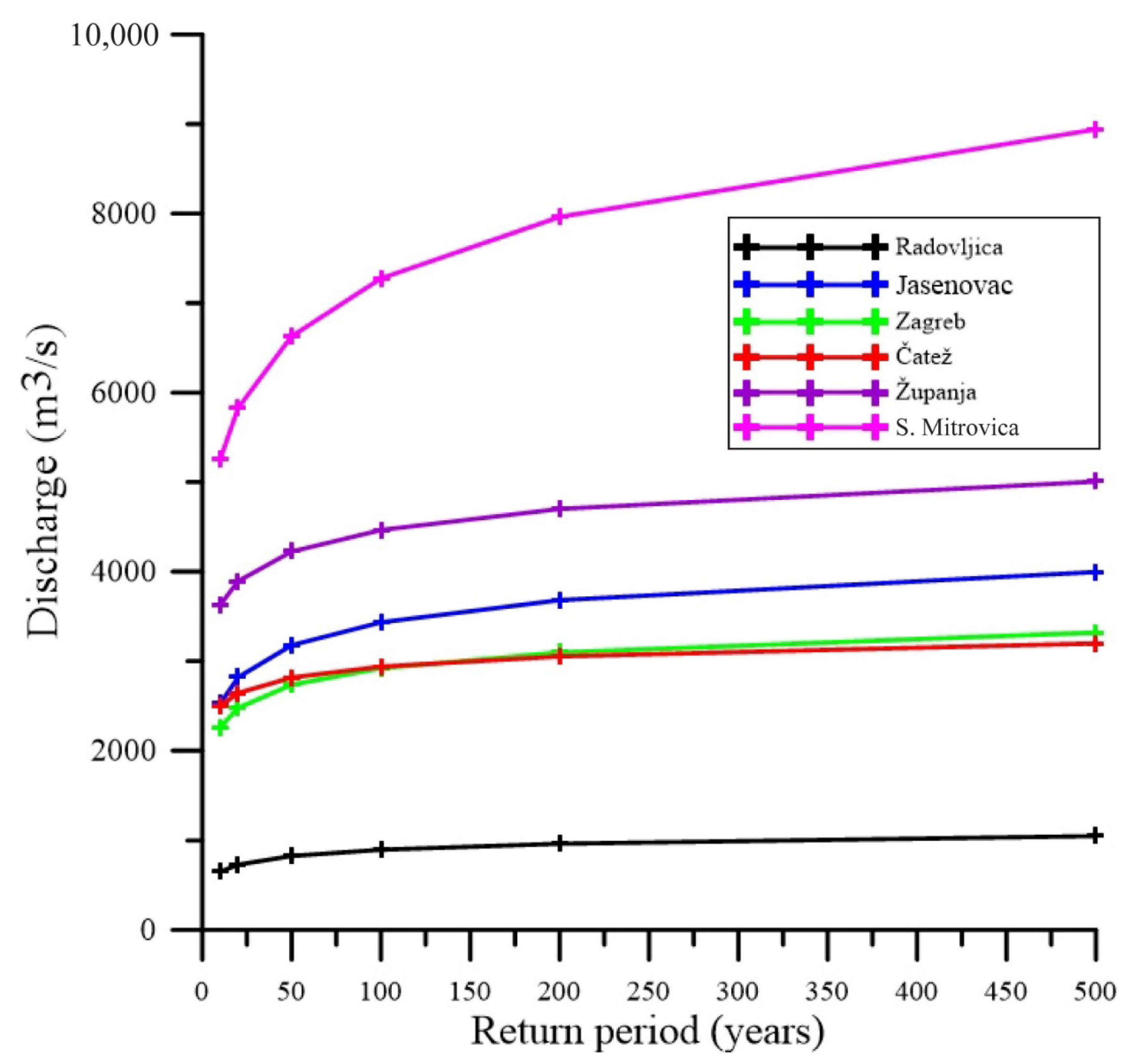
One of the main purposes of FFA is to determine the quantiles (return levels) in the extreme upper end (i.e., flood levels) of the best-fitting distribution. This was achieved by estimating the parameters of the overall best-fitting (i.e., the GEV) distribution for the selected stations. The regional shape parameter is the average of the at-site shape parameters [43]. The return discharge levels for the various stations follow then from the regional shape parameter plus the other at-site GEV parameter estimates (Figure 6).

Figure 6.
Estimated return discharge levels for different return periods for the six selected gauging stations in the Sava River basin.
One of the advantages for using RFFA is that the estimates at a single site can be increased by applying data from other sites within homogeneous region that are confirmed to have similar frequency distribution [43,84]. Application of the L-moments technique is appropriate for increasing the sample size for the RFFA. The L-moments approach simultaneously uses data from several homogeneous basins in a hydrological analysis [85]. Our study shows that this technique is an effective approach for discharge estimation of flood peaks related to the selected return periods in basins with missing data or relatively short time span of data.
6. Conclusions
We employed the FFA and RFFA methods using various theoretical distributions fitted to AMS discharge series from six hydrological stations in the Sava River basin. Our first aim was to determine the best-fitting distributional shape for the various datasets. Using long-term series (1961–2020) with few missing data enabled a robust statistical inference. The homogeneity test confirmed that the investigated area can be considered as homogeneous, so no further subdivision into different basin parts was necessary. Our second aim was to compute regional frequencies of the AMS (i.e., flood risk parameters). For this purpose, quantiles and return levels were estimated at a confidence level of 1 − α = 95%. The results show that the considered distributions (GEV, GLO, Gumbel, LNIII and LPIII) are for most of the stations in good agreement with the test requirement (|Z|<1.96). Overall, the GEV distribution delivered the smallest absolute Z-values, almost uniformly the smallest u-values, and also the regional mean confirms that the GEV is the best-fitting option. Hence, we conclude that the GEV distribution provides the best fit for the Sava River basin.
A trend analysis showed that although the majority of stations (four out of six) exhibit increasing trends, few of the trend estimates are statistically significant. The observed variations between positive and negative trends are thought to be mainly a consequence of modified conditions in the upstream river sections. In such cases, the size of the basin and the degree of human interventions make it difficult to quantify the relationships of climate elements (i.e., the temperature rise) and discharge properties [86]. Model projections suggest a decreasing trend in thickness and duration of the snow cover in the Alpine and Dinaric area in the twenty-first century [55]. These changes must also be taken into consideration for adaptation planning [87]. Particularly important is the observed change at the relatively low elevations (600 to 1300 m) [55].
The results of this study provide helpful information for designers of the various hydraulic structures (levees, bridges, spillways, etc.) and also for policymakers in need of a decision-support tool for flood estimation along the Sava River. The results also enable more robust estimates of design discharges corresponding to different return periods for the design of the hydraulic structures, which could lead to the reduction of the risk of the failure of these structures and to reduce the negative impacts and environmental damages from future flooding.
We provide a short outlook from a practical flood risk protection viewpoint. On the one hand, the underlying datasets are (1) limited in length, (2) limited in time resolution and (3) plagued by measurement errors (e.g., from the water stage–runoff calibrations). This situation leads inevitably to statistical uncertainties of made inferences [63], such as the return levels (Figure 5 and Figure 6). On the other hand, however, the data constitute the best what is, and what will be, available and we believe that the trend analyses and the RFFA methodology (Section 4) are quite capable of taking the data quality into account and provide reliable uncertainty measures. An interesting option for future short-term flood risk protection is usage of modern instrumental, wide-range measurement data, which have the potential to contribute flood information at high spatial resolution. This has been attempted recently for Bangladesh with the help of satellite data [88] and Iran with the help of remote-sensing data [89]. Finally, in a rational world, where science informs politicians—what decisions should follow from the risk curves such as for the return period (Figure 5 and Figure 6)? Answer: it depends, namely on the financial resources and the political instruments at the disposal of the decision makers. If money is available and also the will to protect from damages, these curves may help to find out at which geographical place a good return (in terms of prevented losses) can be expected from a made investment. Scientists should be ready to respond if asked for advice by decision makers.
Author Contributions
Conceptualization, I.L. and B.B.; methodology, I.L and M.M. (Manfred Mudelsee); software, I.L., M.M. (Minučer Mesaroš) and M.M. (Manfred Mudelsee); validation, formal analysis, investigation and resources, I.L., B.B. and M.M. (Manfred Mudelsee); data curation, I.L., B.B., M.Š. and D.P.; writing—original draft preparation, I.L. and M.M. (Manfred Mudelsee); writing—review and editing, M.M. (Manfred Mudelsee); visualization, I.L. and M.M. (Minučer Mesaroš); supervision, project administration and funding acquisition, B.B. All authors have read and agreed to the published version of the manuscript.
Funding
This research was supported by ExtremeClimTwin project, which has received funding from the European Union’s Horizon 2020 research and innovation programme under grant agreement No 952384.
Institutional Review Board Statement
Not applicable.
Informed Consent Statement
Not applicable.
Data Availability Statement
The AMS data presented in this study are openly available at Zenodo (DOI: 10.5281/zenodo.6906445)].
Acknowledgments
The discharge data used in the present study were obtained from the Slovenian Environment Agency (ARSO), Croatian Meteorological and Hydrological Service (DHMZ) and Republic Hydrometeorological Service of Serbia (RHMZ). We thank Professor Rob Wilby (Loughborough University, United Kingdom) for a critical read of the manuscript. We are grateful for all three detailed and constructive reviews received on the initial submission.
Conflicts of Interest
The authors declare no conflict of interest.
Appendix A. Mathematical Formulas for the Distribution Functions
We briefly write down the CDFs for the five theoretical distributions fitted to the data. If there exist several variants of a CDF, then we only consider those with nonzero shape parameter and right-skewness. Note that there exist various ways of expressing the formulas and various parameter notations. More details, such as general descriptions and numerical approximations, can be found in standard textbooks [43,63,90,91,92].
The GEV distribution has the following CDF:
where the parameters satisfy the following conditions: 1 + ξ(x − µ)/σ > 0, −∞ < µ < ∞, σ > 0 and −∞ < ξ < ∞.
The GLO distribution has the following CDF:
where the parameters satisfy the following conditions: –∞ < µ < ∞ and σ > 0.
The Gumbel distribution has the following CDF:
where the parameters satisfy the following conditions: −∞ < µ < ∞ and σ > 0.
The LNIII distribution has no explicit analytical form for the CDF. However, the probability density function, fX(x), where
is given by
where ln(·) is the natural logarithm of an argument and the parameters satisfy following conditions: −∞ < µ < ∞, x > µ and σ > 0.
The LPIII distribution has the following CDF:
where
is the incomplete gamma function, Γ(·) is the gamma function of an argument and the parameters satisfy the following conditions: −∞ < α < ∞, −∞ < µ < ∞ and σ > 0.
References
- Adikari, Y.; Yoshitani, J. Global Trends in Water-Related Disasters: An Insight for Policymakers; United Nations Educational, Scientific and Cultural Organization: Paris, France, 2009. [Google Scholar]
- Pandžić, K.; Trninić, D.; Likso, T.; Bošnjak, T. Long-term variations in water balance components for Croatia. Theor. Appl. Climatol. 2009, 95, 39–51. [Google Scholar] [CrossRef]
- Fischer, S.; Schumann, A.H. Multivariate flood frequency analysis in large river basins considering tributary impacts and flood types. Water Resour. Res. 2021, 57, e2020WR029029. [Google Scholar] [CrossRef]
- Kundzewicz, Z.W. (Ed.) Changes in Flood Risk in Europe; IAHS Press: Wallingford, UK, 2012. [Google Scholar]
- Mudelsee, M.; Börngen, M.; Tetzlaff, G.; Grünewald, U. Extreme floods in central Europe over the past 500 years: Role of cyclone pathway “Zugstrasse Vb.”. J. Geophys. Res. Atmos. 2004, 109, D23101. [Google Scholar] [CrossRef] [Green Version]
- Dottori, F.; Szewczyk, W.; Ciscar, J.-C.; Zhao, F.; Alfieri, L.; Hirabayashi, Y.; Bianchi, A.; Mongelli, I.; Frieler, K.; Betts, R.A.; et al. Increased human and economic losses from river flooding with anthropogenic warming. Nat. Clim. Change 2018, 8, 781–786. [Google Scholar] [CrossRef]
- Ward, P.J.; de Perez, E.C.; Dottori, F.; Jongman, B.; Luo, T.; Safaie, S.; Uhlemann-Elmer, S. The need for mapping, modeling, and predicting flood hazard and risk at the global scale. In Global Flood Hazard: Applications in Modeling, Mapping, and Forecasting; Schumann, G.J.-P., Bates, P.D., Apel, H., Aronica, G.T., Eds.; American Geophysical Union: Washington, DC, USA, 2018; pp. 1–15. [Google Scholar]
- Black, A.R. Major flooding and increased flood frequency in Scotland since 1988. Phys. Chem. Earth 1995, 20, 463–468. [Google Scholar] [CrossRef]
- Brázdil, R.; Kundzewicz, Z.W.; Benito, G.; Demarée, G.; Macdonald, N.; Roald, L.A. Historical floods in Europe in the past millennium. In Changes in Flood Risk in Europe; Kundzewicz, Z.W., Ed.; IAHS Press: Wallingford, UK, 2012; pp. 121–166. [Google Scholar]
- Disse, M.; Engel, H. Flood events in the Rhine basin: Genesis, influences and mitigation. Nat. Hazards 2001, 23, 271–290. [Google Scholar] [CrossRef]
- Jongman, B.; Hochrainer-Stigler, S.; Feyen, L.; Aerts, J.C.J.H.; Mechler, R.; Botzen, W.J.W.; Bouwer, L.M.; Pflug, G.; Rojas, R.; Ward, P.J. Increasing stress on disaster-risk finance due to large floods. Nat. Clim. Change 2014, 4, 264–268. [Google Scholar] [CrossRef]
- Mikhailova, M.V.; Mikhailov, V.N.; Morozov, V.N. Extreme hydrological events in the Danube river basin over the last decades. Water Resour. 2012, 39, 161–179. [Google Scholar] [CrossRef]
- Oblak, J.; Kobold, M.; Šraj, M. The influence of climate change on discharge fluctuations in Slovenian rivers. Acta Geogr. Slov. 2021, 61, 155–169. [Google Scholar] [CrossRef]
- Olsen, J.R.; Stedinger, J.R.; Matalas, N.C.; Stakhiv, E.Z. Climate variability and flood frequency estimation for the upper Mississippi and lower Missouri rivers. J. Am. Water Resour. Assoc. 1999, 35, 1509–1523. [Google Scholar] [CrossRef]
- Osterkamp, W.R.; Friedman, J.M. The disparity between extreme rainfall events and rare floods—with emphasis on the semi-arid American West. Hydrol. Process. 2000, 14, 2817–2829. [Google Scholar] [CrossRef]
- Paprotny, D.; Sebastian, A.; Morales-Nápoles, O.; Jonkman, S.N. Trends in flood losses in Europe over the past 150 years. Nat. Comm. 2018, 9, 1985. [Google Scholar] [CrossRef]
- Petrow, T.; Merz, B. Trends in flood magnitude, frequency and seasonality in Germany in the period 1951–2002. J. Hydrol. 2009, 371, 129–141. [Google Scholar] [CrossRef] [Green Version]
- Robson, A.J. Evidence for trends in UK flooding. Phil. Trans. R. Soc. Lond. A 2002, 360, 1327–1343. [Google Scholar] [CrossRef]
- de Roo, A.; Odijk, M.; Schmuck, G.; Koster, E.; Lucieer, A. Assessing the effects of land use changes on floods in the Meuse and Oder catchment. Phys. Chem. Earth Part B 2001, 26, 593–599. [Google Scholar] [CrossRef]
- Ulbrich, U.; Fink, A. The January 1995 flood in Germany: Meteorological versus hydrological causes. Phys. Chem. Earth 1995, 20, 439–444. [Google Scholar] [CrossRef]
- WMO. State of the Global Climate 2020; World Meteorological Organization: Geneva, Switzerland, 2021. [Google Scholar]
- Blöschl, G.; Hall, J.; Viglione, A.; Perdigão, R.A.P.; Parajka, J.; Merz, B.; Lun, D.; Arheimer, B.; Aronica, G.T.; Bilibashi, A.; et al. Changing climate both increases and decreases European river floods. Nature 2019, 573, 108–111. [Google Scholar] [CrossRef]
- Stocker, T.F.; Qin, D.; Plattner, G.-K.; Tignor, M.M.B.; Allen, S.K.; Boschung, J.; Nauels, A.; Xia, Y.; Bex, V.; Midgley, P.M. (Eds.) Climate Change 2013: The Physical Science Basis. Working Group I Contribution to the Fifth Assessment Report of the Intergovernmental Panel on Climate Change; Cambridge University Press: Cambridge, UK, 2013. [Google Scholar]
- Tapoglou, E.; Vozinaki, A.E.; Tsanis, I. Climate change impact on the frequency of hydrometeorological extremes in the island of Crete. Water 2019, 11, 587. [Google Scholar] [CrossRef] [Green Version]
- Wilcox, C.; Vischel, T.; Panthou, G.; Bodian, A.; Blanchet, J.; Descroix, L.; Quantin, G.; Cassé, C.; Tanimoun, B.; Kone, S. Trends in hydrological extremes in the Senegal and Niger Rivers. J. Hydrol. 2018, 566, 531–545. [Google Scholar] [CrossRef]
- Christensen, J.H.; Christensen, O.B. Severe summertime flooding in Europe. Nature 2003, 421, 805–806. [Google Scholar] [CrossRef]
- Palmer, T.N.; Räisänen, J. Quantifying the risk of extreme seasonal precipitation events in a changing climate. Nature 2002, 415, 512–514. [Google Scholar] [CrossRef]
- Gavrilović, L.; Milanović Pešić, A.; Urošev, M. A hydrological analysis of the greatest floods in Serbia in the 1960-2010 period. Carpathian J. Earth Environ. Sci. 2012, 7, 107–116. [Google Scholar]
- Bezak, N.; Brilly, M.; Šraj, M. Flood frequency analyses, statistical trends and seasonality analyses of discharge data: A case study of the Litija station on the Sava River. J. Flood Risk Manag. 2016, 9, 154–168. [Google Scholar] [CrossRef]
- Ilnicki, P.; Farat, R.; Górecki, K.; Lewandowski, P. Impact of climatic change on river discharge in the driest region of Poland. Hydrol. Sci. J. 2014, 59, 1117–1134. [Google Scholar] [CrossRef] [Green Version]
- Leščešen, I.; Dolinaj, D. Regional flood frequency analysis of the Pannonian Basin. Water 2019, 11, 193. [Google Scholar] [CrossRef] [Green Version]
- Šraj, M.; Bezak, N. Comparison of time trend- and precipitation-informed models for assessing design discharges in variable climate. J. Hydrol. 2020, 589, 125374. [Google Scholar] [CrossRef]
- England, J.F., Jr.; Cohn, T.A.; Faber, B.A.; Stedinger, J.R.; Thomas, W.O., Jr.; Veilleux, A.G.; Kiang, J.E.; Mason, R.R., Jr. Guidelines for Determining Flood Flow Frequency—Bulletin 17C (ver. 1.1), Book 4, Chapter B5; U.S. Geological Survey: Reston, VA, USA, 2019.
- Thorarinsdottir, T.L.; Hellton, K.H.; Steinbakk, G.H.; Schlichting, L.; Engeland, K. Bayesian regional flood frequency analysis for large catchments. Water Resour. Res. 2018, 54, 6929–6947. [Google Scholar] [CrossRef] [Green Version]
- Cassalho, F.; Beskow, S.; de Mello, C.R.; de Moura, M.M. Regional flood frequency analysis using L-moments for geographically defined regions: An assessment in Brazil. J. Flood Risk Manag. 2019, 12, e12453. [Google Scholar] [CrossRef]
- Leščešen, I.; Šraj, M.; Pantelić, M.; Dolinaj, D. Assessing the impact of climate on annual and seasonal discharges at the Sremska Mitrovica station on the Sava River, Serbia. Water Supply 2022, 22, 195–207. [Google Scholar] [CrossRef]
- Šraj, M.; Bezak, N.; Brilly, M. Bivariate flood frequency analysis using the copula function: A case study of the Litija station on the Sava River. Hydrol. Process. 2014, 29, 225–238. [Google Scholar] [CrossRef]
- Bormann, H.; Pinter, N.; Elfert, S. Hydrological signatures of flood trends on German rivers: Flood frequencies, flood heights and specific stages. J. Hydrol. 2011, 404, 50–66. [Google Scholar] [CrossRef]
- Hailegeorgis, T.T.; Alfredsen, K. Regional flood frequency analysis and prediction in ungauged basins including estimation of major uncertainties for mid-Norway. J. Hydrol. Reg. Stud. 2017, 9, 104–126. [Google Scholar] [CrossRef]
- Rutkowska, A.; Żelazny, M.; Kohnová, S.; Łyp, M.; Banasik, K. Regional L-moment-based flood frequency analysis in the upper Vistula River basin, Poland. Pure Appl. Geophys. 2017, 174, 701–721. [Google Scholar] [CrossRef]
- Leščešen, I.; Urošev, M.; Dolinaj, D.; Pantelić, M.; Telbisz, T.; Varga, G.; Savić, S.; Milošević, D. Regional flood frequency analysis based on L-moment approach (case study Tisza River basin). Water Resour. 2019, 46, 853–860. [Google Scholar] [CrossRef]
- Morlot, M.; Brilly, M.; Šraj, M. Characterisation of the floods in the Danube River basin through flood frequency and seasonality analysis. Acta Hydrotech. 2019, 32, 73–89. [Google Scholar] [CrossRef]
- Hosking, J.R.M.; Wallis, J.R. Regional Frequency Analysis: An Approach Based on L-Moments; Cambridge University Press: Cambridge, UK, 1997. [Google Scholar]
- Kar, K.K.; Yang, S.-K.; Lee, J.-H.; Khadim, F.K. Regional frequency analysis for consecutive hour rainfall using L-moments approach in Jeju Island, Korea. Geoenviron. Disasters 2017, 4, 18. [Google Scholar] [CrossRef]
- Stadtherr, L.; Coumou, D.; Petoukhov, V.; Petri, S.; Rahmstorf, S. Record Balkan floods of 2014 linked to planetary wave resonance. Sci. Adv. 2016, 2, e1501428. [Google Scholar] [CrossRef] [Green Version]
- Vidmar, A.; Globevnik, L.; Koprivšek, M.; Sečnik, M.; Zabret, K.; Durović, B.; Anzeljc, D.; Kastelic, J.; Kobold, M.; Sušnik, M.; et al. The Bosna River floods in May 2014. Nat. Hazards Earth Syst. Sci. 2016, 16, 2235–2246. [Google Scholar] [CrossRef] [Green Version]
- Plavšić, J.; Vladiković, D.; Despotović, J. Floods in the Sava River basin in May 2014. In Monitoring, Modelling and Early Warning of Extreme Events Triggered by Heavy Rainfall; Ferrari, E., Versace, P., Eds.; University of Calabria: Cosenza, Italy, 2014; pp. 241–251. [Google Scholar]
- United Nations (UN); European Union (EU); World Bank (WB). Serbia Floods 2014; United Nations; European Union; World Bank: Belgrade, Serbia, 2014. [Google Scholar]
- Plavšić, J.; Vladiković, D.; Despotović, J. Hydrometeorological aspects of floods in May 2014 in the Sava River Basin and in Serbia. Voda Sanit. Teh. 2014, 44, 21–33. [Google Scholar]
- International Commission for the Protection of the Danube River (ICPDR); International Sava River Basin Commission (ISRBC). Floods in May 2014 in the Sava River Basin: Brief Overview of Key Events and Lessons Learned; International Commission for the Protection of the Danube River: Vienna, Austria, 2015. [Google Scholar]
- Ladan, T. Hrvatska Enciklopedija, Mrežno Izdanje; Sava; Leksikogr. Zavod Miroslav Krleža [Miroslav Krleža Institute of Lexicography]: Zagreb, Croatia, 2021. [Google Scholar]
- Dolšak, D.; Bezak, N.; Šraj, M. Temporal characteristics of rainfall events under three climate types in Slovenia. J. Hydrol. 2016, 541, 1395–1405. [Google Scholar] [CrossRef]
- Lavtar, K.; Bezak, N.; Šraj, M. Rainfall-runoff modeling of the nested non-homogeneous Sava River sub-catchments in Slovenia. Water 2020, 12, 128. [Google Scholar] [CrossRef] [Green Version]
- Ulaga, P.; Kobold, M.; Frantar, F. Trends of river discharges in Slovenia. IOP Conf. Ser. Earth Environ. Sci. 2008, 4, 012030. [Google Scholar] [CrossRef]
- Čanjevac, I.; Orešić, D. Changes in discharge regimes of rivers in Croatia. Acta Geogr. Slov. 2018, 58, 7–18. [Google Scholar] [CrossRef] [Green Version]
- Mudelsee, M. Statistical Analysis of Climate Extremes; Cambridge University Press: Cambridge, UK, 2020. [Google Scholar]
- Urošev, M.; Dolinaj, D.; Leščešen, I. Hydrological droughts in the Južna Morava River basin (Serbia). Geogr. Pannon. 2016, 20, 197–207. [Google Scholar] [CrossRef] [Green Version]
- Gumbel, E.J. Statistics of Extremes; Columbia University Press: New York, NY, USA, 1958. [Google Scholar]
- Bickel, P. Robust estimation. In Encyclopedia of Statistical Sciences; Kotz, S., Johnson, N.L., Read, C.B., Eds.; Wiley: New York, NY, USA, 1988; Volume 8, pp. 157–163. [Google Scholar]
- Bezak, N.; Brilly, M.; Šraj, M. Comparison between the peaks-over-threshold method and the annual maximum method for flood frequency analysis. Hydrol. Sci. J. 2014, 59, 959–977. [Google Scholar] [CrossRef] [Green Version]
- Faulkner, D.; Warren, S.; Spencer, P.; Sharkey, P. Can we still predict the future from the past? Implementing non-stationary flood frequency analysis in the UK. J. Flood Risk Manag. 2020, 13, e12582. [Google Scholar] [CrossRef] [Green Version]
- Kousar, S.; Khan, A.R.; Hassan, M.U.; Noreen, Z.; Bhatti, S.H. Some best-fit probability distributions for at-site flood frequency analysis of the Ume River. J. Flood Risk Manag. 2020, 13, e12640. [Google Scholar] [CrossRef]
- Mudelsee, M. Climate Time Series Analysis: Classical Statistical and Bootstrap Methods, 2nd ed.; Springer: Cham, Switzerland, 2014. [Google Scholar]
- Fisher, R.A.; Tippett, L.H.C. Limiting forms of the frequency distribution of the largest or smallest member of a sample. Math. Proc. Camb. Phil. Soc. 1928, 24, 180–190. [Google Scholar] [CrossRef]
- Fréchet, M. Sur la loi probabilité de l’écart maximum. Ann. Soc. Pol. Math. 1927, 6, 93–116. [Google Scholar]
- Karim, F.; Hasan, M.; Marvanek, S. Evaluating annual maximum and partial duration series for estimating frequency of small magnitude floods. Water 2017, 9, 481. [Google Scholar] [CrossRef] [Green Version]
- Zhang, Z.; Stadnyk, T.A. Investigation of attributes for identifying homogeneous flood regions for regional flood frequency analysis in Canada. Water 2020, 12, 2570. [Google Scholar] [CrossRef]
- Zalnezhad, A.; Rahman, A.; Vafakhah, M.; Samali, B.; Ahamed, F. Regional flood frequency analysis using the FCM-ANFIS algorithm: A case study in South-eastern Australia. Water 2022, 14, 1608. [Google Scholar] [CrossRef]
- St. George, S.; Mudelsee, M. The weight of the flood-of-record in flood frequency analysis. J. Flood Risk Manag. 2019, 12, e12512. [Google Scholar] [CrossRef] [Green Version]
- Robson, A.; Reed, D. Flood Estimation Handbook, Volume 3, Statistical Procedures for Flood Frequency Estimation; Centre for Ecology & Hydrology: Wallingford, UK, 1999. [Google Scholar]
- Bogdanowicz, E.; Kochanek, K.; Strupczewski, W.G. The weighted function method: A handy tool for flood frequency analysis or just a curiosity? J. Hydrol. 2018, 559, 209–221. [Google Scholar] [CrossRef]
- Rahman, A.S.; Rahman, A.; Zaman, M.A.; Haddad, K.; Ahsan, A.; Imteaz, M. A study on selection of probability distributions for at-site flood frequency analysis in Australia. Nat. Hazards 2013, 69, 1803–1813. [Google Scholar] [CrossRef]
- Hosking, J.R.M.; Wallis, J.R. Some statistics useful in regional frequency analysis. Water Resour. Res. 1993, 29, 271–281. [Google Scholar] [CrossRef]
- Peel, M.C.; Wang, Q.J.; Vogel, R.M.; McMahon, T.A. The utility of L-moment ratio diagrams for selecting a regional probability distribution. Hydrol. Sci. J. 2001, 46, 147–155. [Google Scholar] [CrossRef]
- Stephens, M.A. Kolmogorov–Smirnov-type tests of fit. In Encyclopedia of Statistical Sciences; Kotz, S., Johnson, N.L., Read, C.B., Eds.; Wiley: New York, NY, USA, 1983; Volume 4, pp. 398–402. [Google Scholar]
- Urošev, M.; Leščešen, I.; Štrbac, D.; Dolinaj, D. Extreme hydrological situations on Danube River—Case study Bezdan hydrological station (Serbia). In Sustainable Hydraulics in the Era of Global Change; Erpicum, S., Dewals, B., Archambeau, P., Pirotton, M., Eds.; Taylor & Francis: London, UK, 2016; p. 137. [Google Scholar]
- Bhat, M.S.; Alam, A.; Ahmad, B.; Kotlia, B.S.; Farooq, H.; Taloor, A.K.; Ahmad, S. Flood frequency analysis of river Jhelum in Kashmir basin. Quat. Int. 2019, 507, 288–294. [Google Scholar] [CrossRef]
- Kovacevic-Majkic, J.; Urosev, M. Trends of mean annual and seasonal discharges of rivers in Serbia. J. Geogr. Inst. Jovan Cvijic 2014, 64, 143–160. [Google Scholar] [CrossRef]
- Arnell, N.W.; Gosling, S.N. The impacts of climate change on river flow regimes at the global scale. J. Hydrol. 2013, 486, 351–364. [Google Scholar] [CrossRef]
- Schneider, C.; Laizé, C.L.R.; Acreman, M.C.; Flörke, M. How will climate change modify river flow regimes in Europe? Hydrol. Earth Syst. Sci. 2013, 17, 325–339. [Google Scholar] [CrossRef] [Green Version]
- Stagl, J.C.; Hattermann, F.F. Impacts of climate change on the hydrological regime of the Danube River and its tributaries using an ensemble of climate scenarios. Water 2015, 7, 6139–6172. [Google Scholar] [CrossRef]
- Ahmad, I.; Fawad, M.; Akbar, M.; Abbas, A.; Zafar, H. Regional frequency analysis of annual peak flows in Pakistan using linear combination of order statistics. Pol. J. Environ. Stud. 2016, 25, 2255–2264. [Google Scholar] [CrossRef]
- Zabret, K.; Brilly, M. Hydrological regionalisation of flood frequency analyses in Slovenia. Acta Hydrotech. 2014, 27, 139–156. [Google Scholar]
- Saf, B. Regional flood frequency analysis using L-moments for the West Mediterranean region of Turkey. Water Resour Manag. 2009, 23, 531–551. [Google Scholar] [CrossRef]
- Mosaffaie, J. Comparison of two methods of regional flood frequency analysis by using L-moments. Water Resour. 2015, 42, 313–321. [Google Scholar] [CrossRef]
- Čanjevac, I.; Orešić, D. Contemporary changes of mean annual and seasonal river discharges in Croatia. Hrvat. Geogr. Glas. 2015, 77, 7–27. [Google Scholar] [CrossRef] [Green Version]
- Steiger, R. The impact of snow scarcity on ski tourism: An analysis of the record warm season 2006/2007 in Tyrol (Austria). Tour. Rev. 2011, 66, 4–13. [Google Scholar] [CrossRef]
- Aziz, M.A.; Moniruzzaman, M.; Tripathi, A.; Hossain, M.I.; Ahmed, S.; Rahaman, K.R.; Rahman, F.; Ahmed, R. Delineating flood zones upon employing synthetic aperture data for the 2020 flood in Bangladesh. Earth Syst. Environ. 2022. [Google Scholar] [CrossRef]
- Farhadi, H.; Najafzadeh, M. Flood risk mapping by remote sensing data and random forest technique. Water 2021, 13, 3115. [Google Scholar] [CrossRef]
- Johnson, N.L.; Kotz, S.; Balakrishnan, N. Continuous Univariate Distributions, 2nd ed.; Wiley: New York, NY, USA, 1994; Volume 1. [Google Scholar]
- Johnson, N.L.; Kotz, S.; Balakrishnan, N. Continuous Univariate Distributions, 2nd ed.; Wiley: New York, NY, USA, 1995; Volume 2. [Google Scholar]
- Singh, V.P. Entropy-Based Parameter Estimation in Hydrology; Springer: Dordrecht, The Netherlands, 1998. [Google Scholar]
Publisher’s Note: MDPI stays neutral with regard to jurisdictional claims in published maps and institutional affiliations. |
© 2022 by the authors. Licensee MDPI, Basel, Switzerland. This article is an open access article distributed under the terms and conditions of the Creative Commons Attribution (CC BY) license (https://creativecommons.org/licenses/by/4.0/).

