
Building Carbon Emission Scenario Prediction Using STIRPAT and GA-BP Neural Network Model


Abstract
:1. Introduction
2. Literature Review
3. Research Methods and Models
3.1. Gray Correlation Method
3.2. STIRPAT Model
3.3. GA-BP Neural Network Model
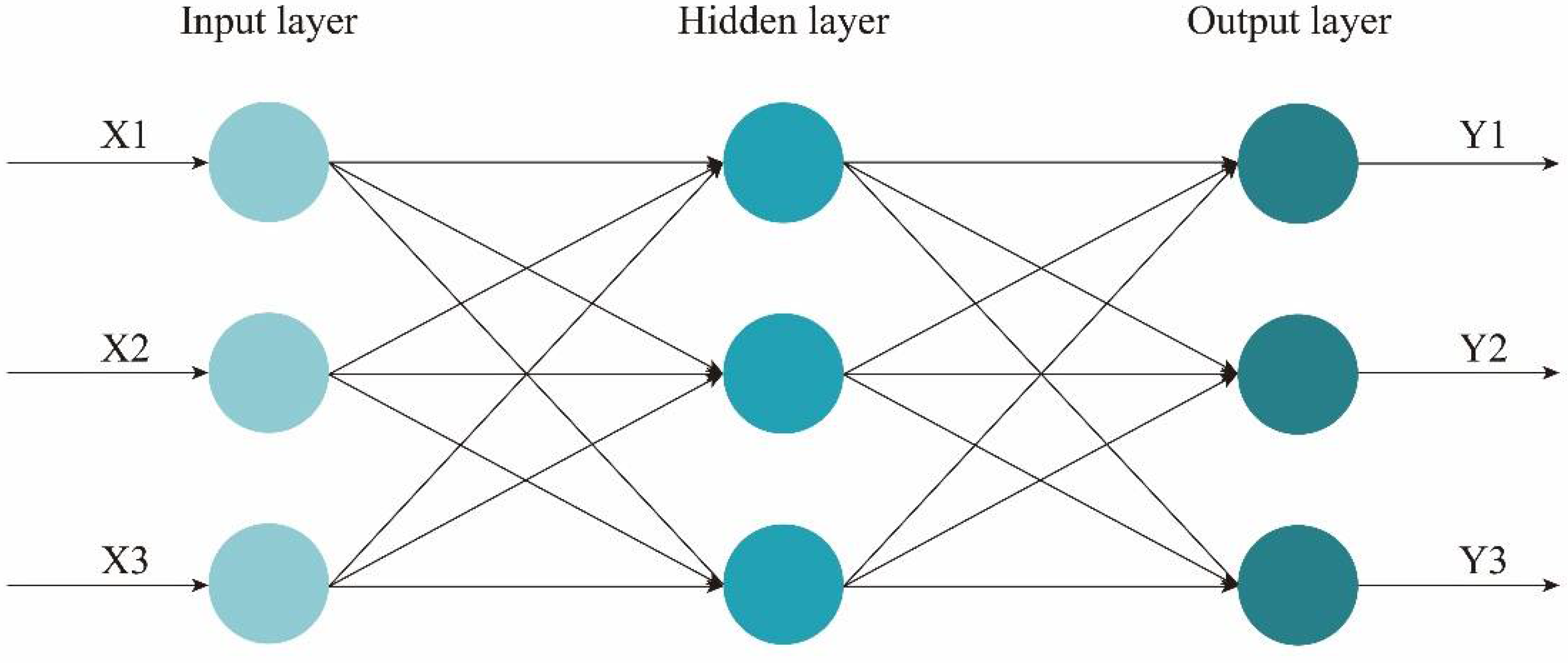
3.3.1. BP Neural Network
3.3.2. Genetic Algorithm
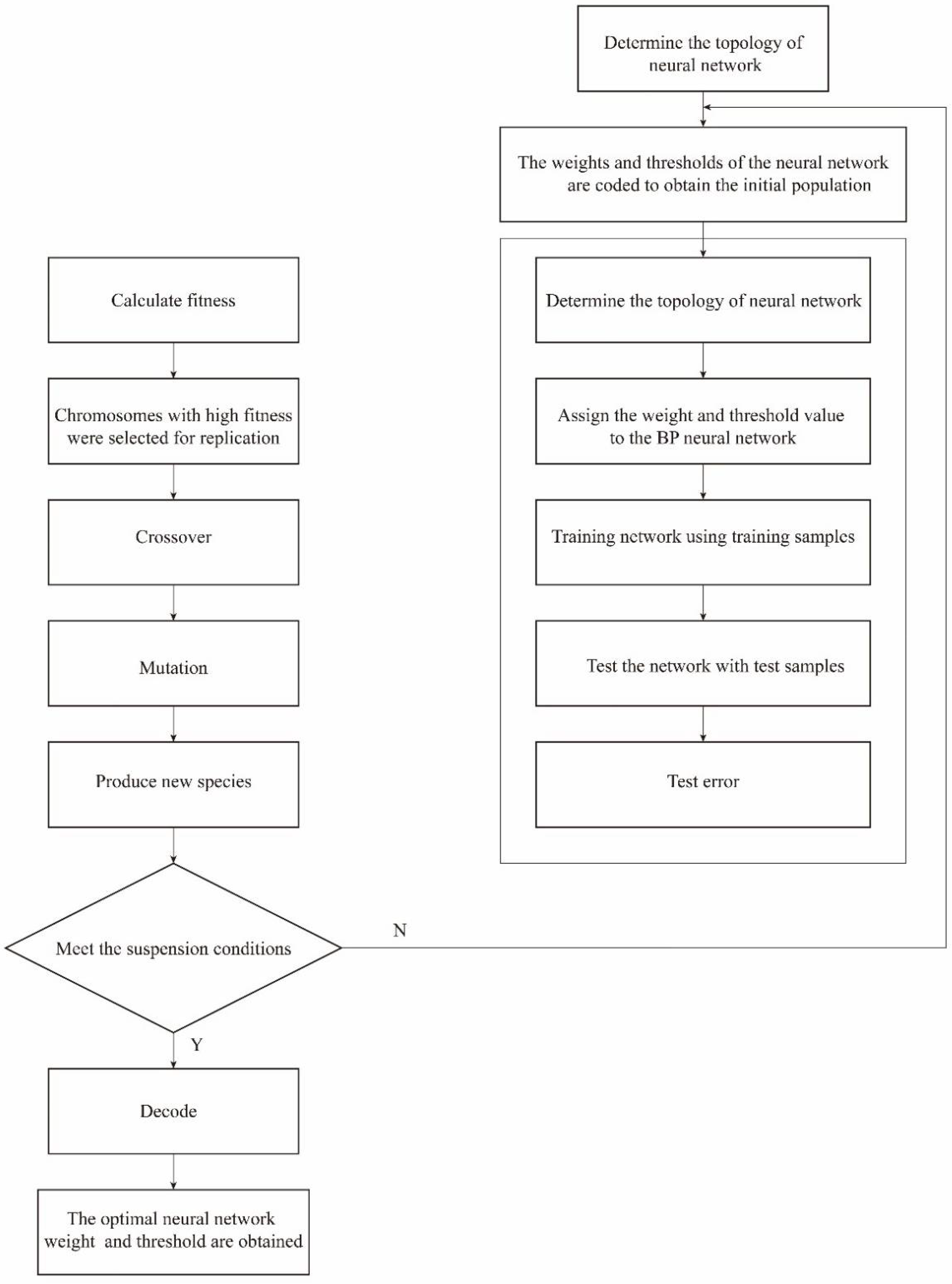
3.3.3. Genetic Algorithm to Optimize BP Neural Network
3.4. Ridge Regression
4. Model Construction and Data Analysis
4.1. Multicollinearity Analysis
4.2. Ridge Regression Analysis
5. Carbon Emission Scenario Setting for Buildings in Jiangsu Province
6. GA-BP Model Validation and Prediction of Building Carbon Emissions
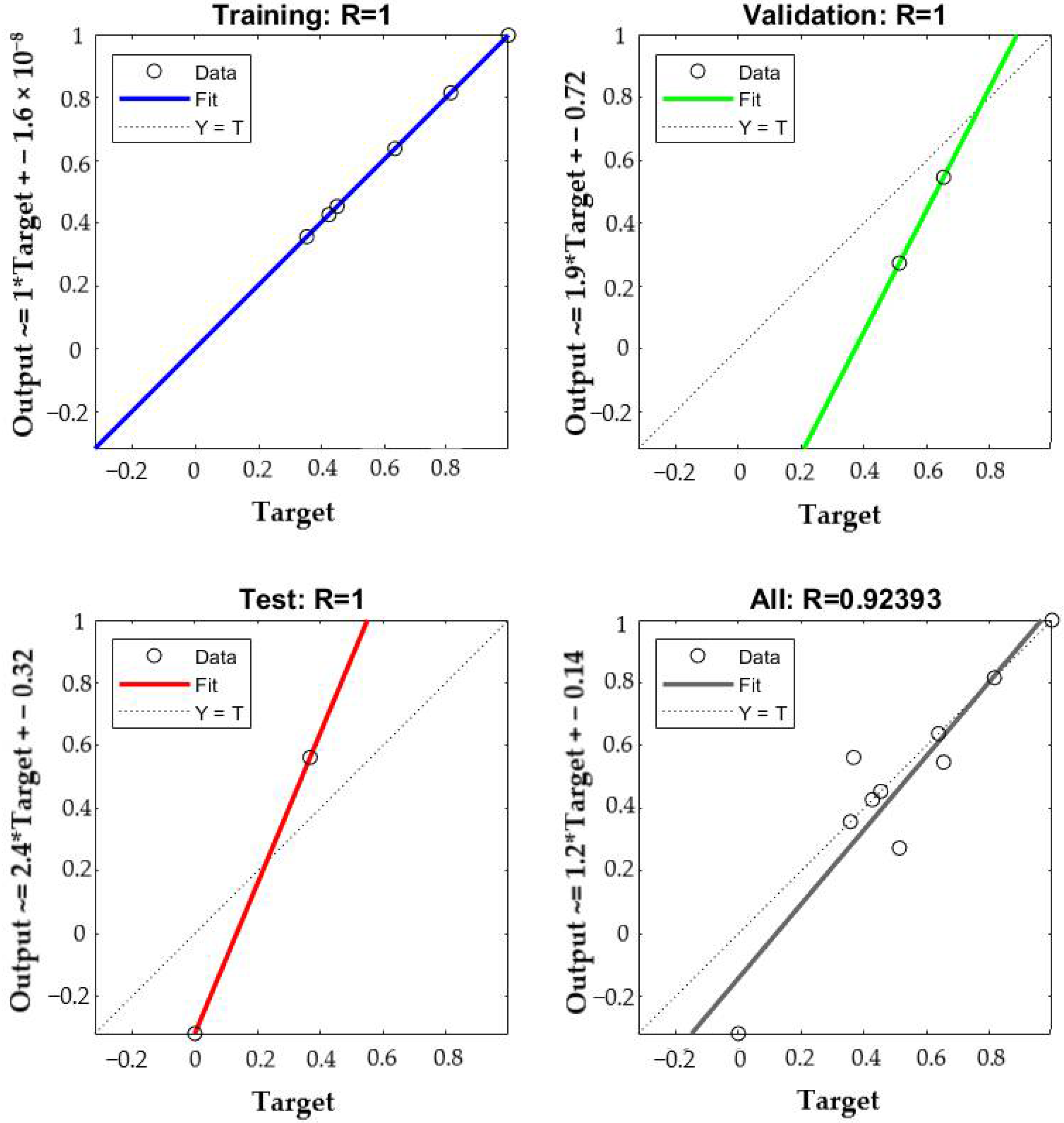
6.1. GA-BP Model Validation
6.2. Scenario Prediction Results
7. Conclusions
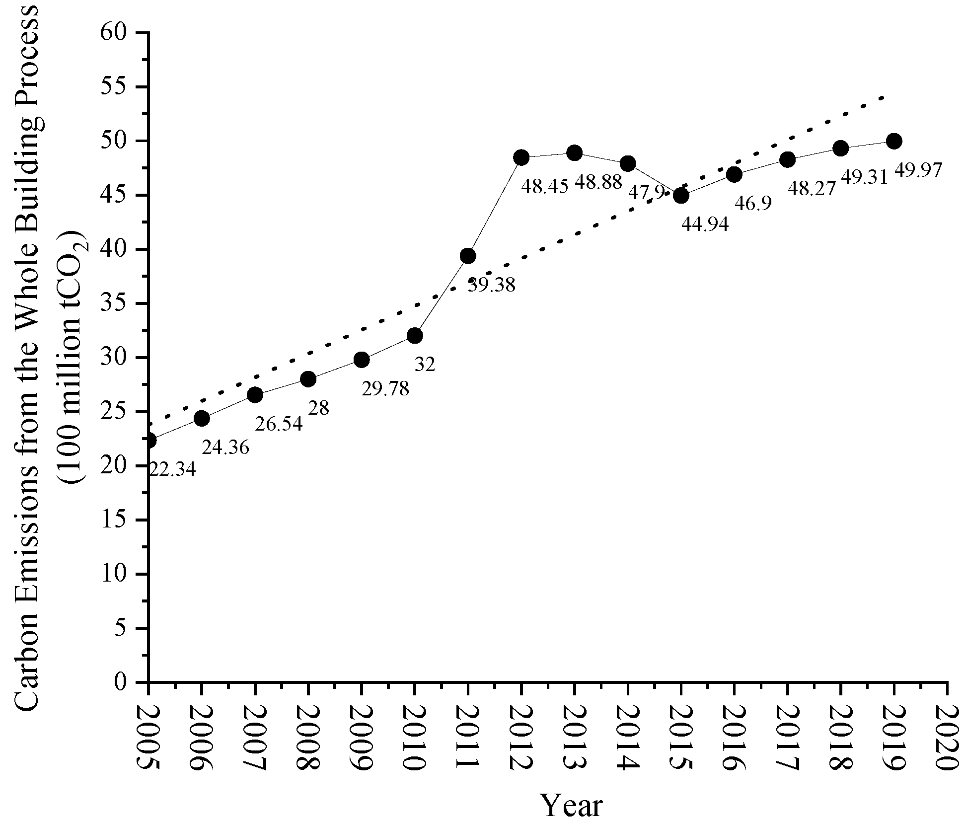
- (1)
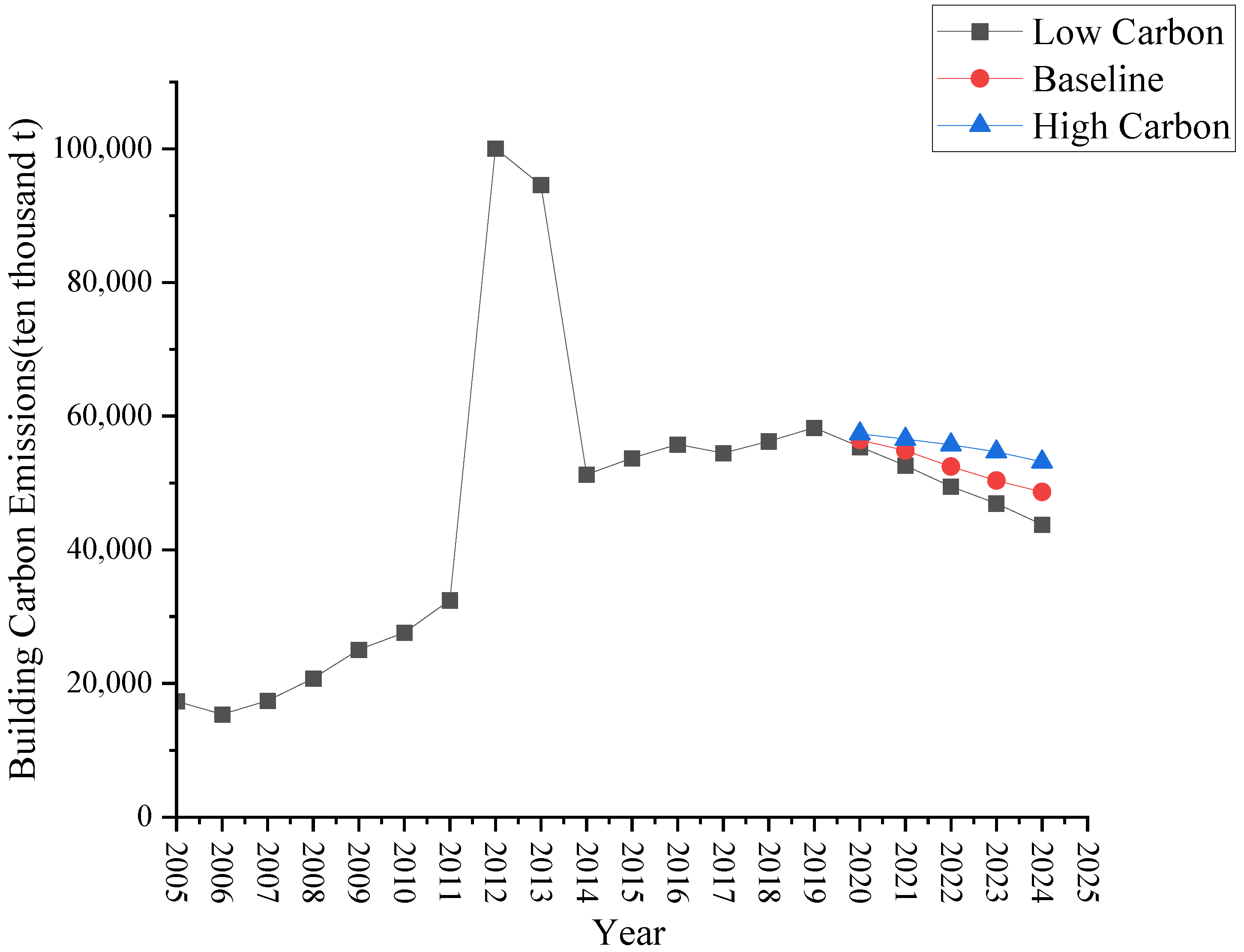
- The growth of whole life cycle carbon emissions of buildings in Jiangsu Province from 2005 to 2019 is about 409,476,000 tons, peaking in 2012 and gradually decreasing and leveling off afterward. This shows that the construction industry in Jiangsu Province has the initial carbon peak conditions.
- (2)
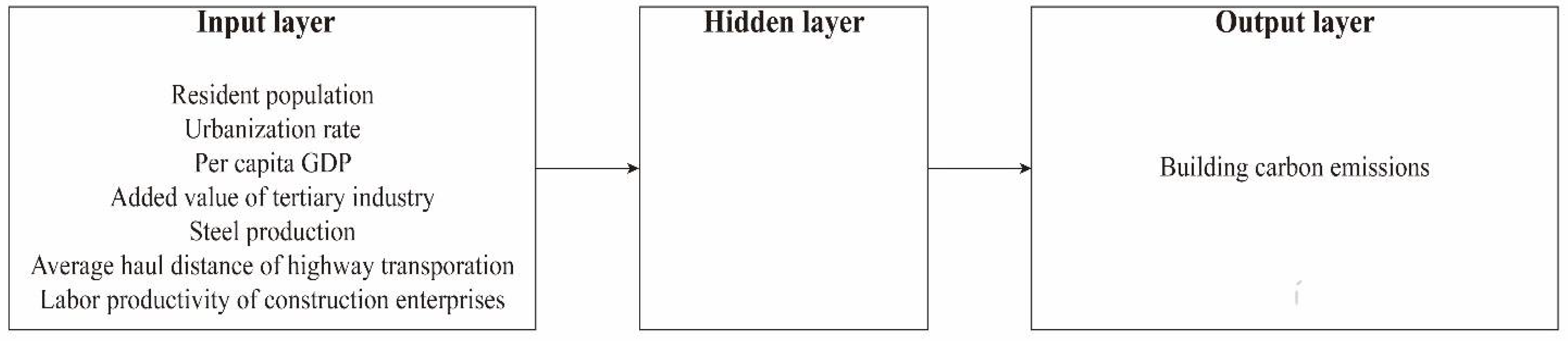
- Resident population, urbanization rate, steel production, average road transportation distance, and construction enterprise labor productivity have a catalytic effect on construction carbon emissions; GDP per capita and value-added of the tertiary industry have a suppressive effect. Among them, steel production has a significant catalytic effect on carbon emissions. Therefore, in the process of carbon emission reduction in the construction industry of Jiangsu Province, it is necessary to reduce the use of steel as much as possible and switch to the use of new energy-saving and emission-reducing materials as an alternative.
- (3)
- According to the elasticity coefficient, the absolute value of the coefficient for the resident population is the largest, which indicates that the resident population is the most sensitive factor affecting the change of whole life cycle carbon emission of buildings in Jiangsu province. That is, the change in the number of resident population per unit has the greatest influence on the change of life-cycle carbon emissions of buildings in Jiangsu Province.
- (4)
- The prediction results show that the overall trend of carbon emissions from 2020 to 2024 is decreasing. In addition, under the high carbon scenario and the low carbon scenario, there is a large difference in the carbon emissions of buildings between the two, indicating that there is still more room for carbon emission reduction in the construction industry in Jiangsu Province.
Author Contributions
Funding
Institutional Review Board Statement
Informed Consent Statement
Data Availability Statement
Acknowledgments
Conflicts of Interest
References
- Climate Change 2022: Mitigation of Climate Change. 2022. Available online: https://www.ipcc.ch/report/ar6/wg3/ (accessed on 4 April 2022).
- China Building Energy Consumption Research Report [R/OL]. Xiamen: Energy Consumption Statistics Professional Committee. 2020. Available online: https://www.cabee.org/site/content/24021.html (accessed on 15 April 2022).
- China Building Energy Consumption Research Report [R/OL]. Shanghai: Energy Consumption Statistics Professional Committee. 2018. Available online: https://www.cabee.org/site/content/22960.html (accessed on 14 April 2022).
- Qingyi, W. Research on statistics and calculation of building energy consumption in China. Energy Conserv. Environ. 2007, 8, 9–10. [Google Scholar]
- Xuyi, L.; Shun, Z.; Junghan, B. Nonlinear analysis of technological innovation and electricity generation on carbon dioxide emissions in China. J. Clean. Prod. 2022, 343, 131021. [Google Scholar]
- Ming, M.; Dongxiao, N. Modeling CO2 emissions from fossil fuel combustion using the logistic equation. Energy 2011, 36, 3355–3359. [Google Scholar] [CrossRef]
- Takako, W.; Eric, Z. The impact of electricity market reform and subnational climate policy on carbon dioxide emissions across the United States: A path analysis. Renew. Sustain. Energy Rev. 2021, 149, 111337. [Google Scholar]
- Mingming, Z.; Zikun, Y.; Liyun, L.; Dequn, Z. Impact of renewable energy investment on carbon emissions in China—An empirical study using a nonparametric additive regression model. Sci. Total Environ. 2021, 785, 147109. [Google Scholar]
- Ozcan, B.; Ulucak, R. An empirical investigation of nuclear energy consumption and carbon dioxide (CO2) emission in India: Bridging IPAT and EKC hypotheses. Nucl. Eng. Technol. 2021, 53, 2056–2065. [Google Scholar]
- Alex, O.A.; Emmanuel, B.B. Modelling carbon emission intensity: Application of artificial neural network. J. Clean. Prod. 2019, 225, 833–856. [Google Scholar]
- Guangyue, X.; Peter, S.; Hualiu, Y. Determining China’s CO2 emissions peak with a dynamic nonlinear artificial neural network approach and scenario analysis. Energy Policy 2019, 128, 752–762. [Google Scholar]
- Ru, F.; Xufeng, Z.; Aaron, B.; Tingting, Z.; Jin-Song, L.; Xiang-Zhou, M. Achieving China’s carbon neutrality: Predicting driving factors of CO2 emission by artificial neural network. J. Clean. Prod. 2022, 362, 132331. [Google Scholar]
- Dongxiao, N.; Keke, W.; Jing, W.; Lijie, S.; Yi, L.; Xiaomin, X.; Xiaolong, Y. Can China achieve its 2030 carbon emissions commitment? Scenario analysis based on an improved general regression neural network. J. Clean. Prod. 2020, 243, 118558. [Google Scholar]
- Hong, Y.; Qun, R.; Xinyue, H.; Tao, L.; Longyu, S.; Guoqin, Z.; Xinhu, L. Modeling energy-related CO2 emissions from office buildings using general regression neural network. Resour. Conserv. Recycl. 2018, 129, 168–174. [Google Scholar]
- Ziyuan, C.; Yibo, Y.; Simayi, Z.; Shengtian, Y.; Abulimiti, M.; Yuqing, W. Carbon emissions index decomposition and carbon emissions prediction in Xinjiang from the perspective of population-related factors, based on the combination of STIRPAT model and neural network. Environ. Sci. Pollut. Res. 2022, 29, 31781–31796. [Google Scholar] [CrossRef] [PubMed]
- Zhang, Y.; Liu, C.; Chen, L.; Wang, X.; Song, X.; Li, K. Energy-related CO2 emission peaking target and pathways for China’s city: A case study of Baoding City. J. Clean. Prod. 2019, 226, 471–481. [Google Scholar] [CrossRef]
- Yuzhe, W.; Jiahui, S.; Xiaoling, Z.; Martin, S.; Wisheng, L. Reprint of: The impact of urbanization on carbon emissions in developing countries: A Chinese study based on the U-Kaya method. J. Clean. Prod. 2017, 163, S284–S298. [Google Scholar]
- Shaikh, M.S.U.E.; Jakob, N. Energy use and CO2 emissions in the UK universities: An extended Kaya identity analysis. J. Clean. Prod. 2021, 309, 127199. [Google Scholar]
- Lei, W.; Zhenkai, L. Driving forces of national and regional CO2 emissions in China combined IPAT-E and PLS-SEM model. Sci. Total Environ. 2019, 690, 237–247. [Google Scholar]
- Ting, Y.; Ruyin, L.; Hong, C.; Xin, Z. The optimal CO2 emissions reduction path in Jiangsu province: An expanded IPAT approach. Appl. Energy 2013, 112, 1510–1517. [Google Scholar]
- Fangjia, K.; Lihua, H. Impacts of supply-sided and demand-sided policies on innovation in green building technologies: A case study of China. J. Clean. Prod. 2021, 294, 126279. [Google Scholar]
- Xiaoying, W.; Bo, P.; Borong, L. A dynamic life cycle carbon emission assessment on green and non-green buildings in China. Energy Build. 2017, 149, 272–281. [Google Scholar]
- Elaheh, Y.; Mehdi, H.; Mehrbakhsh, N.; Eesa, A.; Sarminah, S.; Marwan, M.; Ala, A.A.; Azida, Z.; Hamsa, D.M.; Liyana, S. Assessment of sustainability indicators for green building manufacturing using fuzzy multi-criteria decision making approach. J. Clean. Prod. 2020, 277, 122905. [Google Scholar]
- Wei, W.; Ze, T.; Wenjia, X.; Yi, R.T.; Yao, D. The influencing factors of China’s green building development: An analysis using RBF-WINGS method. Build. Environ. 2021, 188, 107425. [Google Scholar]
- Nur, K.M.; Che, M.M.I.; Che, K.I.C.I. Top-down bottom-up strategic green building development framework: Case studies in Malaysia. Build. Environ. 2021, 203, 108052. [Google Scholar]
- Al-Sakkaf, A.; Mohammed, A.E.; Mahmoud, S.; Bagchi, A. Studying Energy Performance and Thermal Comfort Conditions in Heritage Buildings: A Case Study of Murabba Palace. Sustainability 2021, 13, 12250. [Google Scholar] [CrossRef]
- Xiaofen, Y.; Dai, F. Review of comprehensive multi-indicator evaluation methods. Stat. Decis. 2004, 11, 119–121. [Google Scholar]
- Pingping, X.; Shuren, C.; Zhuo, Y. Gray correlation analysis of carbon emissions in East China. J. Dalian Univ. Technol. Soc. Sci. 2021, 42, 36–44. [Google Scholar]
- York, R.; Rosa, E.A.; Dietz, T. STIRPAT, IPAT and Impact: Analytic tools for unpacking the driving forces of environmental impacts. Ecol. Econ. 2003, 46, 351–365. [Google Scholar] [CrossRef]
- Zhongmin, X.; Guodong, C. The environmental impact of China’s population and affluence. J. Glaciol. Geocryol. 2005, 5, 767–773. [Google Scholar]
- Hecht-Nielsen, R. Theory of the backpropagation neural network. Int. Jt. Conf. Neural Netw. 1989, 1, 593–605. [Google Scholar]
- Hoerl, A.E.; Kennard, R.W. Ridge regression: Biased estimation fornonorthogonal problems. Technometrics 1970, 12, 55–67. [Google Scholar] [CrossRef]
- China Building Energy Consumption Research Report [R/OL]. Shanghai: Energy Consumption Statistics Professional Committee. 2019. Available online: https://www.cabee.org/site/content/23565.html (accessed on 13 April 2022).
- Weiguang, C.; Xiaohui, L.; Xia, W.; Mingman, C.; Yong, W.; Wei, F. Energy balance sheet based building energy consumption unbundling model and application. Heat. Vent. Air Cond. 2017, 47, 27–34. [Google Scholar]
- Jingjing, W.; Jiajia, W. Characteristics and scenario simulation of carbon emission changes of building operation in Beijing under time series. J. Beijing Univ. Technol. 2022, 48, 220–229. [Google Scholar]


| Year | Steel (Ton) | Cement (Ton) | Glass (Weight Box) | Aluminum (Ton) | Carbon Emissions (Ten Thousand Tons) |
|---|---|---|---|---|---|
| 2005 | 17,176,219 | 72,850,624 | 11,755,245 | 2,135,532 | 12,640.5656 |
| 2006 | 19,365,741 | 82,523,173 | 5,807,113 | 722,611 | 10,412.6537 |
| 2007 | 24,896,823 | 91,657,074 | 6,090,033 | 829,837 | 12,292.2506 |
| 2008 | 30,475,791 | 118,258,785 | 10,392,076 | 780,865 | 14,892.7165 |
| 2009 | 35,532,626 | 152,498,685 | 16,587,859 | 1,079,470 | 18,644.9787 |
| 2010 | 40,618,866 | 157,705,493 | 17,325,388 | 1,301,559 | 20,465.4572 |
| 2011 | 47,989,650 | 182,777,750 | 14,408,094 | 1,738,724 | 24,388.8858 |
| 2012 | 141,117,794 | 754,308,672 | 18,685,165 | 7,466,010 | 89,863.4490 |
| 2013 | 130,393,503 | 316,346,453 | 20,494,290 | 17,162,732 | 83,597.1095 |
| 2014 | 79,550,112 | 245,611,224 | 177,321,086 | 4,397,407 | 41,305.1479 |
| 2015 | 86,746,631 | 271,234,936 | 22,840,682 | 4,136,138 | 42,787.4867 |
| 2016 | 90,703,898 | 245,411,043 | 26,027,869 | 5,243,690 | 44,554.2099 |
| 2017 | 90,562,639 | 241,763,822 | 20,947,231 | 4,293,637 | 42,153.9950 |
| 2018 | 93,709,279 | 239,359,027 | 25,063,438 | 4,493,855 | 43,079.6396 |
| 2019 | 100,465,171 | 257,666,274 | 26,811,036 | 4,107,839 | 44,638.2866 |
| Year | 2005 | 2006 | 2007 | 2008 | 2009 |
|---|---|---|---|---|---|
| Power carbon emission factor (kgCO2/kWh) | 0.8879 | 0.8517 | 0.7798 | 0.7630 | 0.7394 |
| Year | 2010 | 2011 | 2012 | 2013 | 2014 |
| Power carbon emission factor (kgCO2/kWh) | 0.7082 | 0.7475 | 0.7430 | 0.7330 | 0.6972 |
| Year | 2015 | 2016 | 2017 | 2018 | 2019 |
| Power carbon emission factor (kgCO2/kWh) | 0.7007 | 0.6869 | 0.6841 | 0.6556 | 0.6455 |
| Year | 2005 | 2006 | 2007 | 2008 | 2009 |
|---|---|---|---|---|---|
| Thermal carbon emission factor (kg/kg) | 3.1312 | 3.2555 | 3.0945 | 3.1505 | 3.0677 |
| Year | 2010 | 2011 | 2012 | 2013 | 2014 |
| Thermal carbon emission factor (kg/kg) | 2.8153 | 2.9660 | 3.0769 | 3.0159 | 3.0128 |
| Year | 2015 | 2016 | 2017 | 2018 | 2019 |
| Thermal carbon emission factor (kg/kg) | 3.0690 | 3.0149 | 3.0935 | 3.6314 | 3.5692 |
| Year | 2005 | 2006 | 2007 | 2008 | 2009 |
|---|---|---|---|---|---|
| Carbon emissions (Ten Thousand Tons) | 12,640.5656 | 10,412.6537 | 12,292.2506 | 14,892.7165 | 18,644.9787 |
| Year | 2010 | 2011 | 2012 | 2013 | 2014 |
| Carbon emissions (Ten Thousand Tons) | 20,465.4572 | 24,388.8858 | 89,863.4490 | 83,597.1095 | 41,305.1479 |
| Year | 2015 | 2016 | 2017 | 2018 | 2019 |
| Carbon emissions (Ten Thousand Tons) | 42,787.4867 | 44,554.2099 | 42,153.9950 | 43,079.6396 | 44,638.2686 |
| Year | 2005 | 2006 | 2007 | 2008 | 2009 |
|---|---|---|---|---|---|
| Carbon emissions (Ten Thousand Tons) | 113.9471 | 136.4962 | 158.0850 | 197.8498 | 320.4802 |
| Year | 2010 | 2011 | 2012 | 2013 | 2014 |
| Carbon emissions (Ten Thousand Tons) | 345.2539 | 423.8154 | 1664.8701 | 1353.2409 | 978.1925 |
| Year | 2015 | 2016 | 2017 | 2018 | 2019 |
| Carbon emissions (Ten Thousand Tons) | 1013.6430 | 942.5937 | 961.7008 | 941.2930 | 1070.3047 |
| Year | 2005 | 2006 | 2007 | 2008 | 2009 |
|---|---|---|---|---|---|
| Carbon emissions (Ten Thousand Tons) | 4127.0743 | 4359.5150 | 4511.4667 | 5160.9920 | 5570.8610 |
| Year | 2010 | 2011 | 2012 | 2013 | 2014 |
| Carbon emissions (Ten Thousand Tons) | 6139.5220 | 6872.6039 | 7680.1223 | 8694.3287 | 8019.8521 |
| Year | 2015 | 2016 | 2017 | 2018 | 2019 |
| Carbon emissions (Ten Thousand Tons) | 9013.4497 | 9462.6038 | 10,492.9558 | 11,328.2717 | 11,616.3580 |
| Year | 2005 | 2006 | 2007 | 2008 | 2009 |
|---|---|---|---|---|---|
| Carbon emissions * (Ten Thousand Tons) | 449.1982 | 473.4452 | 483.9768 | 499.4249 | 530.2938 |
| Year | 2010 | 2011 | 2012 | 2013 | 2014 |
| Carbon emissions (Ten Thousand Tons) | 648.4856 | 771.1489 | 852.3013 | 944.6358 | 971.8402 |
| Year | 2015 | 2016 | 2017 | 2018 | 2019 |
| Carbon emissions (Ten Thousand Tons) | 901.2428 | 828.8998 | 855.2922 | 901.7684 | 953.4604 |
| Year | Resident Population (Ten Thousand People) | Urbanization Rate (%) | Per Capita GDP (Yuan) | Added Value of Tertiary Industry (Hundred Million Yuan) | Steel Production (Ton) | Average Distance of Highway Transportation (km) | Labor Productivity of Construction Enterprises (Yuan/Person) | Building Carbon Emissions (Ten Thousand Tons) |
|---|---|---|---|---|---|---|---|---|
| 2005 | 7588.24 | 50.5 | 23,984 | 1300.10 | 17,176,219 | 60.18 | 127,657 | 17,330.79 |
| 2006 | 7655.66 | 51.9 | 27,868 | 1284.32 | 19,365,741 | 64.29 | 142,846 | 15,382.11 |
| 2007 | 7723.13 | 53.2 | 33,798 | 1993.99 | 24,896,823 | 65.51 | 160,387 | 17,445.78 |
| 2008 | 7762.48 | 54.3 | 39,967 | 2130.80 | 30,475,791 | 65.60 | 174,742 | 20,750.98 |
| 2009 | 7810.27 | 55.6 | 44,272 | 1754.71 | 35,532,626 | 93.38 | 189,932 | 25,066.61 |
| 2010 | 7869.34 | 60.6 | 52,787 | 3460.14 | 40,618,866 | 93.04 | 207,116 | 27,598.72 |
| 2011 | 8022.99 | 62.0 | 61,464 | 3578.19 | 47,989,650 | 93.41 | 249,338 | 32,456.45 |
| 2012 | 8119.81 | 63.0 | 66,533 | 2610.53 | 141,117,794 | 94.50 | 262,834 | 100,060.74 |
| 2013 | 8192.44 | 64.4 | 72,768 | 3442.75 | 130,393,503 | 172.64 | 282,532 | 94,589.31 |
| 2014 | 8281.09 | 65.7 | 78,711 | 3421.77 | 79,550,112 | 172.87 | 296,918 | 51,275.03 |
| 2015 | 8315.11 | 67.5 | 85,871 | 3757.42 | 86,746,631 | 182.88 | 297,437 | 53,715.82 |
| 2016 | 8381.47 | 68.9 | 92,658 | 4337.88 | 90,703,898 | 182.68 | 304,925 | 55,788.31 |
| 2017 | 8423.50 | 70.2 | 102,202 | 4430.92 | 90,562,639 | 184.45 | 312,383 | 54,463.94 |
| 2018 | 8446.19 | 71.2 | 110,508 | 4235.98 | 93,709,279 | 182.72 | 335,803 | 56,250.97 |
| 2019 | 8469.09 | 72.5 | 116,650 | 3915.58 | 100,465,171 | 196.55 | 363,015 | 58,278.39 |
| Model | Non-Standardized Coefficient | Collinearity Statistics | |||||
|---|---|---|---|---|---|---|---|
| B | Standard Error | Standardization Coefficient | t | Significance | Tolerance | VIF | |
| Constant | −5.646 | 31.242 | −0.181 | 0.862 | |||
| −0.412 | 3.935 | −0.026 | −0.105 | 0.920 | 0.013 | 79.689 | |
| 2.826 | 1.550 | 0.562 | 1.823 | 0.111 | 0.008 | 121.781 | |
| −1.027 | 0.447 | −0.843 | −2.296 | 0.055 | 0.006 | 172.917 | |
| −0.092 | 0.135 | −0.064 | −0.682 | 0.517 | 0.088 | 11.307 | |
| 1.110 | 0.074 | 1.261 | 14.895 | 0.000 | 0.109 | 9.195 | |
| 0.089 | 0.136 | 0.068 | 0.655 | 0.534 | 0.073 | 13.672 | |
| 0.006 | 0.590 | 0.003 | 0.009 | 0.993 | 0.008 | 130.036 | |
| Variance Ratio | ||||||||||
|---|---|---|---|---|---|---|---|---|---|---|
| Dimension | Characteristic Value | Condition Index | Constant | lnP | lnC | lnG | lnT | lnS | lnR | lnL |
| 1 | 7.993 | 1.000 | 0.00 | 0.00 | 0.00 | 0.00 | 0.00 | 0.00 | 0.00 | 0.00 |
| 2 | 0.006 | 36.337 | 0.00 | 0.00 | 0.00 | 0.00 | 0.00 | 0.00 | 0.07 | 0.00 |
| 3 | 0.001 | 122.863 | 0.00 | 0.00 | 0.00 | 0.00 | 0.30 | 0.00 | 0.24 | 0.00 |
| 4 | 0.000 | 168.490 | 0.00 | 0.00 | 0.00 | 0.00 | 0.05 | 0.42 | 0.10 | 0.00 |
| 5 | 7.258 × 10⁻⁵ | 331.866 | 0.00 | 0.00 | 0.01 | 0.08 | 0.42 | 0.21 | 0.28 | 0.00 |
| 6 | 7.421 × 10⁻⁶ | 1037.830 | 0.00 | 0.00 | 0.63 | 0.08 | 0.04 | 0.09 | 0.04 | 0.16 |
| 7 | 3.574 × 10⁻⁶ | 1495.421 | 0.00 | 0.00 | 0.13 | 0.79 | 0.01 | 0.27 | 0.03 | 0.84 |
| 8 | 1.233 × 10⁻⁷ | 8050.731 | 0.99 | 1.00 | 0.22 | 0.04 | 0.19 | 0.01 | 0.25 | 0.00 |
| K = 0.127 | Non-Standardized Coefficient | Standardization Coefficient | t | p | R2 | Adjusted R2 | F | |
|---|---|---|---|---|---|---|---|---|
| B | Standard Error | Beta | ||||||
| constant | −11.544 | 9.752 | - | −1.184 | 0.275 | 0.944 | 0.889 | 17.001 (0.001 ***1) |
| lnP | 0.877 | 1.146 | 0.056 | 0.765 | 0.469 | |||
| lnC | 0.18 | 0.309 | 0.036 | 0.581 | 0.580 | |||
| lnG | −0.004 | 0.073 | −0.004 | −0.061 | 0.953 | |||
| lnT | −0.091 | 0.161 | −0.063 | −0.561 | 0.592 | |||
| lnS | 0.639 | 0.1 | 0.726 | 6.402 | 0.000 ***1 | |||
| lnR | 0.057 | 0.145 | 0.044 | 0.396 | 0.704 | |||
| lnL | 0.207 | 0.115 | 0.112 | 1.801 | 0.115 | |||
| Scenario Pattern | Rate of Change (%) | ||||||
|---|---|---|---|---|---|---|---|
| Population Size | Urbanization Rate | Per Capita GDP | Added-Value of Tertiary Industry | Steel Production | Average Haul Distance of Highway Transportation | Labor Productivity of Construction Enterprises | |
| Low carbon | 0.70 | 1.25 | 10.5 | 9.5 | 18 | 9.5 | 6.5 |
| Standard | 0.75 | 1.3 | 10 | 9 | 20 | 10 | 7 |
| High carbon | 0.80 | 1.35 | 9.5 | 8.5 | 22 | 10.5 | 7.5 |
Publisher’s Note: MDPI stays neutral with regard to jurisdictional claims in published maps and institutional affiliations. |
© 2022 by the authors. Licensee MDPI, Basel, Switzerland. This article is an open access article distributed under the terms and conditions of the Creative Commons Attribution (CC BY) license (https://creativecommons.org/licenses/by/4.0/).
Share and Cite
Zhang, S.; Huo, Z.; Zhai, C. Building Carbon Emission Scenario Prediction Using STIRPAT and GA-BP Neural Network Model. Sustainability 2022, 14, 9369. https://doi.org/10.3390/su14159369
Zhang S, Huo Z, Zhai C. Building Carbon Emission Scenario Prediction Using STIRPAT and GA-BP Neural Network Model. Sustainability. 2022; 14(15):9369. https://doi.org/10.3390/su14159369
Chicago/Turabian StyleZhang, Sensen, Zhenggang Huo, and Chencheng Zhai. 2022. "Building Carbon Emission Scenario Prediction Using STIRPAT and GA-BP Neural Network Model" Sustainability 14, no. 15: 9369. https://doi.org/10.3390/su14159369
APA StyleZhang, S., Huo, Z., & Zhai, C. (2022). Building Carbon Emission Scenario Prediction Using STIRPAT and GA-BP Neural Network Model. Sustainability, 14(15), 9369. https://doi.org/10.3390/su14159369