
A Practical and Sustainable Approach to Determining the Deployment Priorities of Automatic Vehicle Identification Sensors


Abstract
:1. Introduction
1.1. Background
1.2. Literature Review
1.3. Research Gaps and Contributions
2. Problem Description and Preliminaries
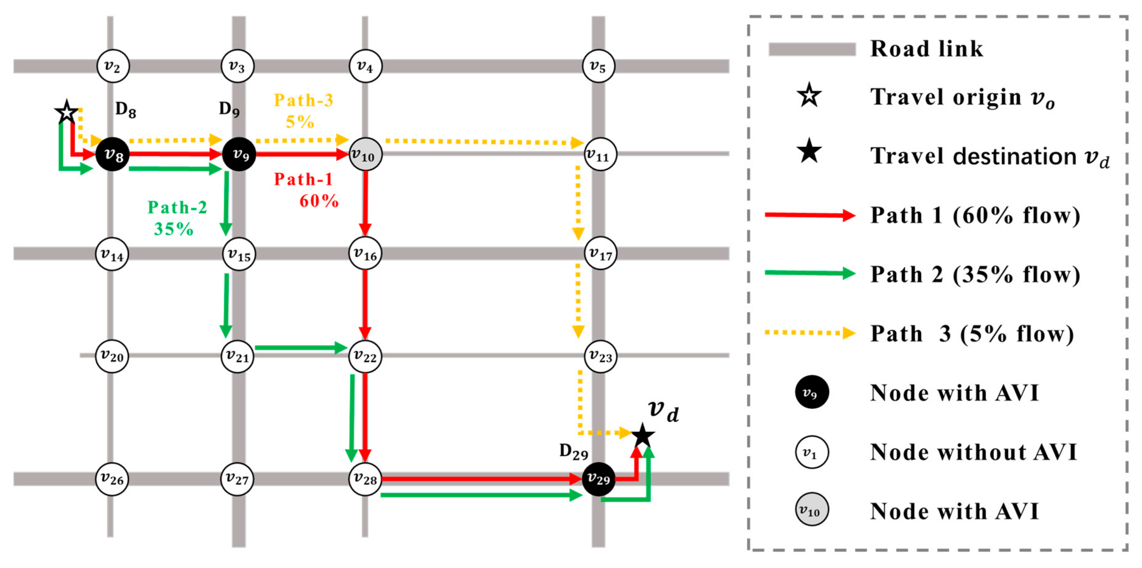
2.1. Problem Description and Assumptions
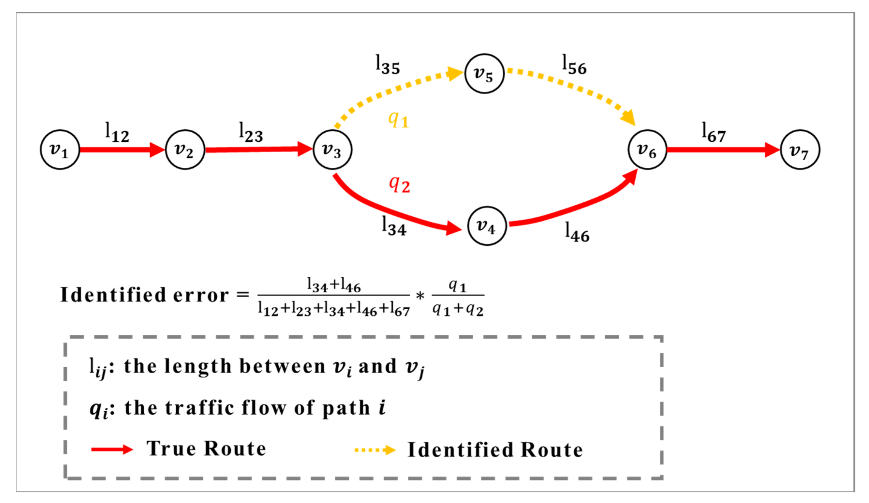
2.2. Preliminary Representation and Traditional Region-Level BPM
3. Model Formulation and Methodology
3.1. Random-Walk Method
3.1.1. Transferring Probability Calculation
3.1.2. Simulation Process
| Algorithm 1: The pseudo-code for the random walk | |
| Input: The surveyed OD matrix, observed trajectory data of the vehicles Output: The path set | |
| 1: | Initialization of and in , the length threshold |
| 2: | Calculate the transferring probability between each pair of nodes; |
| 3: | fordo |
| 4: | initialize to null and add into ; walking agent begins at ; ; |
| 5: | while the total length of does not exceed and the walking agent is not at do |
| 6: | select one of the agent’s adjacent nodes according to the |
| 7: | if is not a repeated or circular path do |
| 8: | add the selected adjacent node into ; |
| 9: | else do |
| 10: | select another one of the agent’s adjacent nodes according to the , return to line 7; |
| 11: | end if |
| 12: | let walking agent move to the last added node; |
| 13: | return |
| 14: | end for |
3.2. Formulating the P-BPM of Each Simulated Path
3.2.1. Problem Restatement
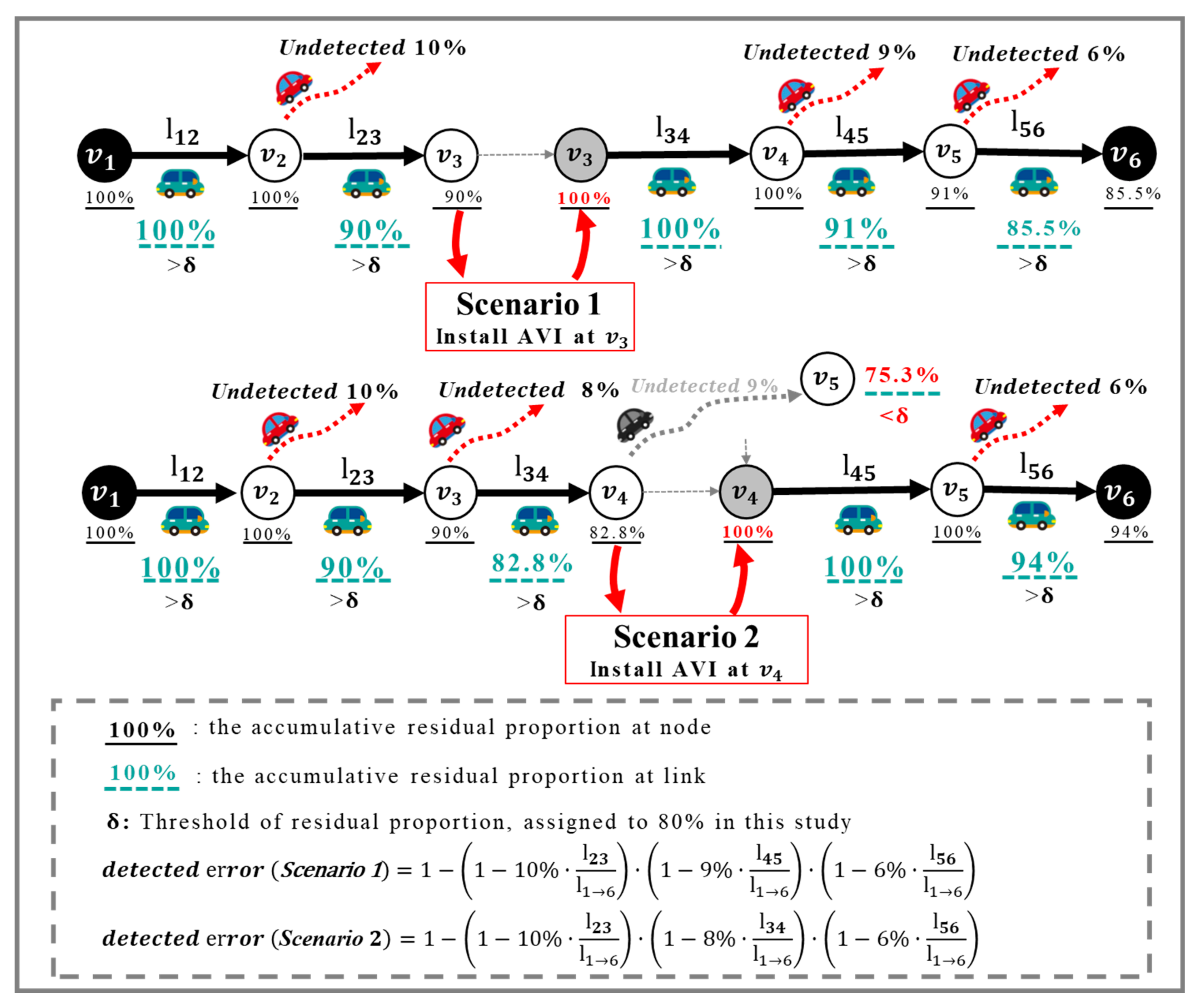
3.2.2. Formulating the P-BPM
3.3. Calculating the Deployment Score
4. Experiments
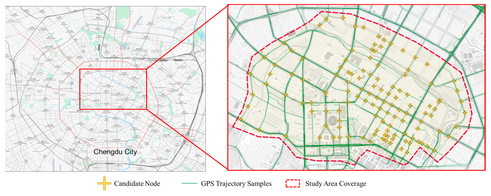
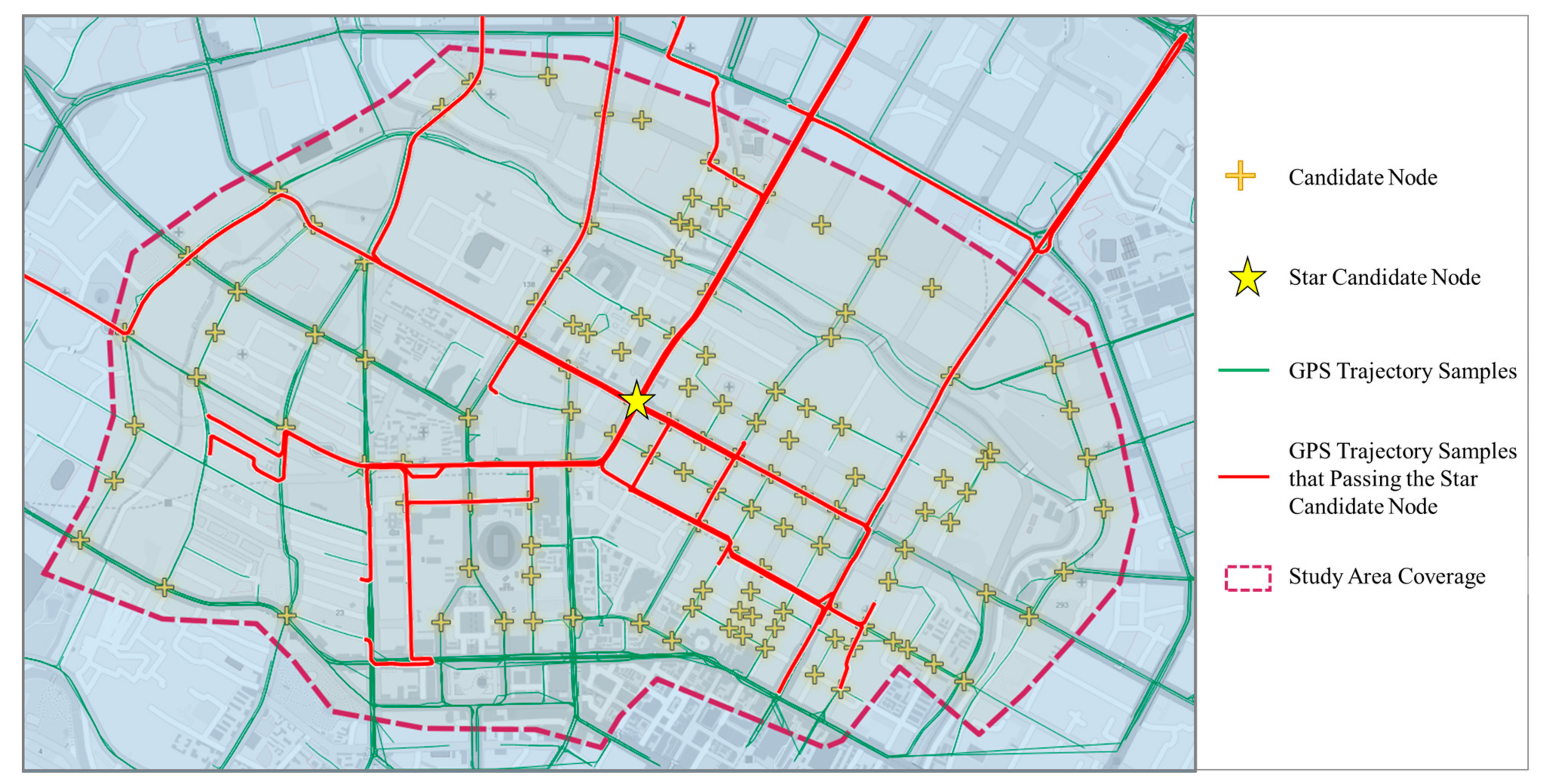
4.1. Dataset
4.2. Evaluation Methodology
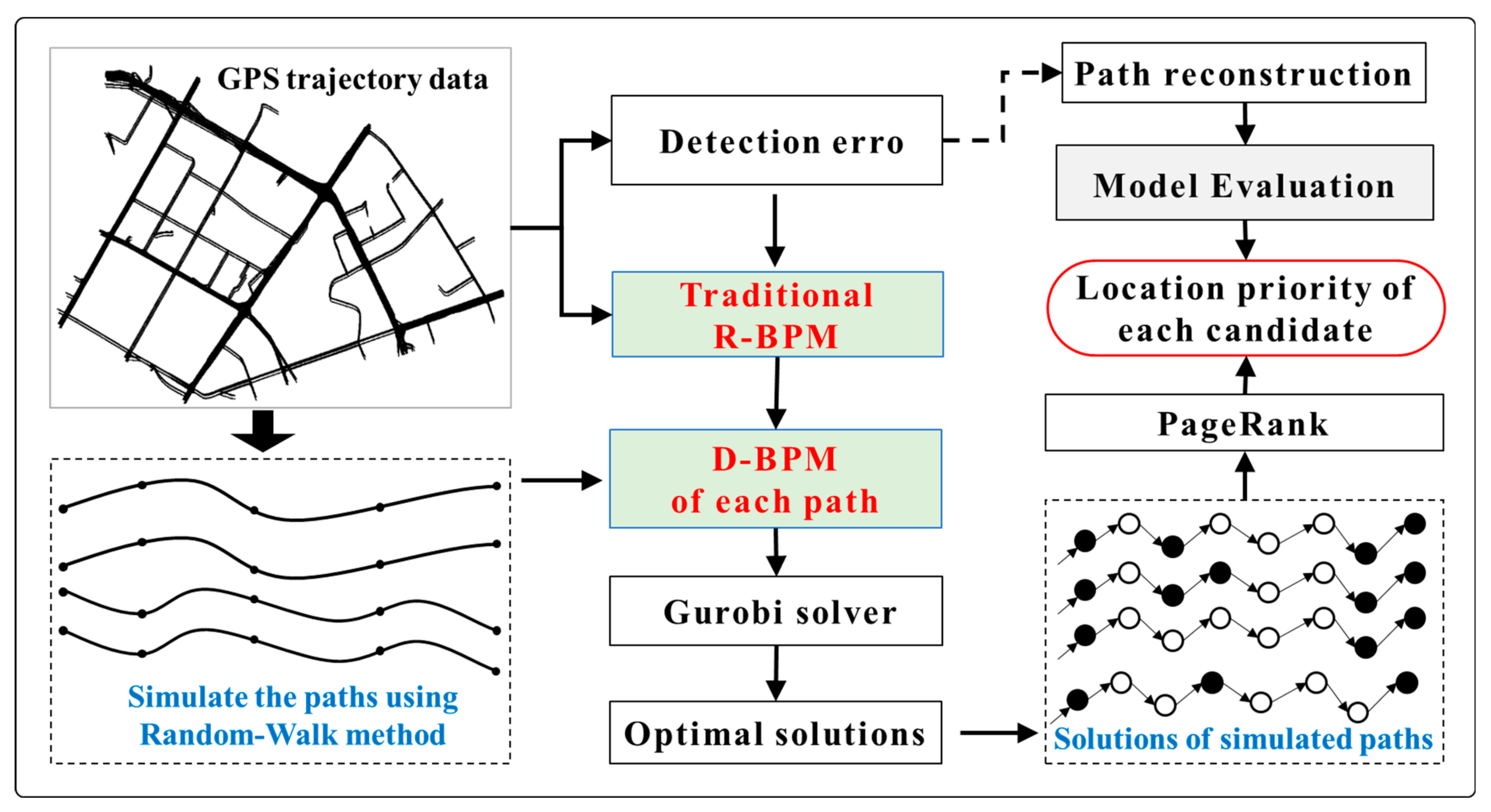
4.2.1. Implementation Procedure
| Algorithm 2: The pseudo-code for inferring the whole detected path | |
| Input: The candidate graph , , and of each candidate node Output: | |
| 1: | Initialize and from the road map and , respectively |
| 2: | |
| 3: | for do |
| 4: | initialize from , = |
| 5: | for each segment from to in do |
| 6: | if is not adjacent to do |
| 7: | remove the path to from |
| 8: | remove the path to from |
| 9: | calculate the total value of the nodes in except and |
| 10: | calculate the total value of the nodes in except and |
| 11: | if do |
| 12: | insert to between and as |
| 13: | else do |
| 14: | insert to between and as |
| 15: | end if |
| 16: | end if |
| 17: | end for |
| 18: | return |
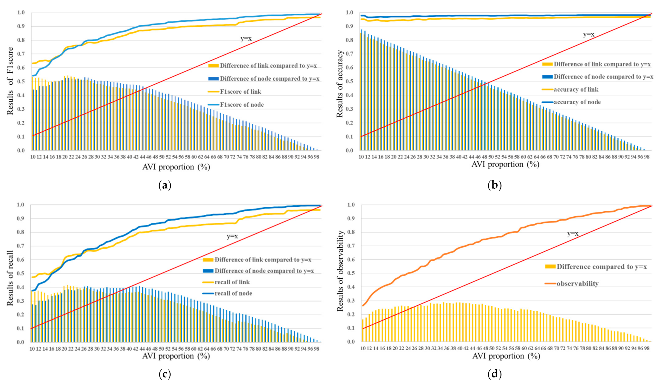
4.2.2. Performance Metrics
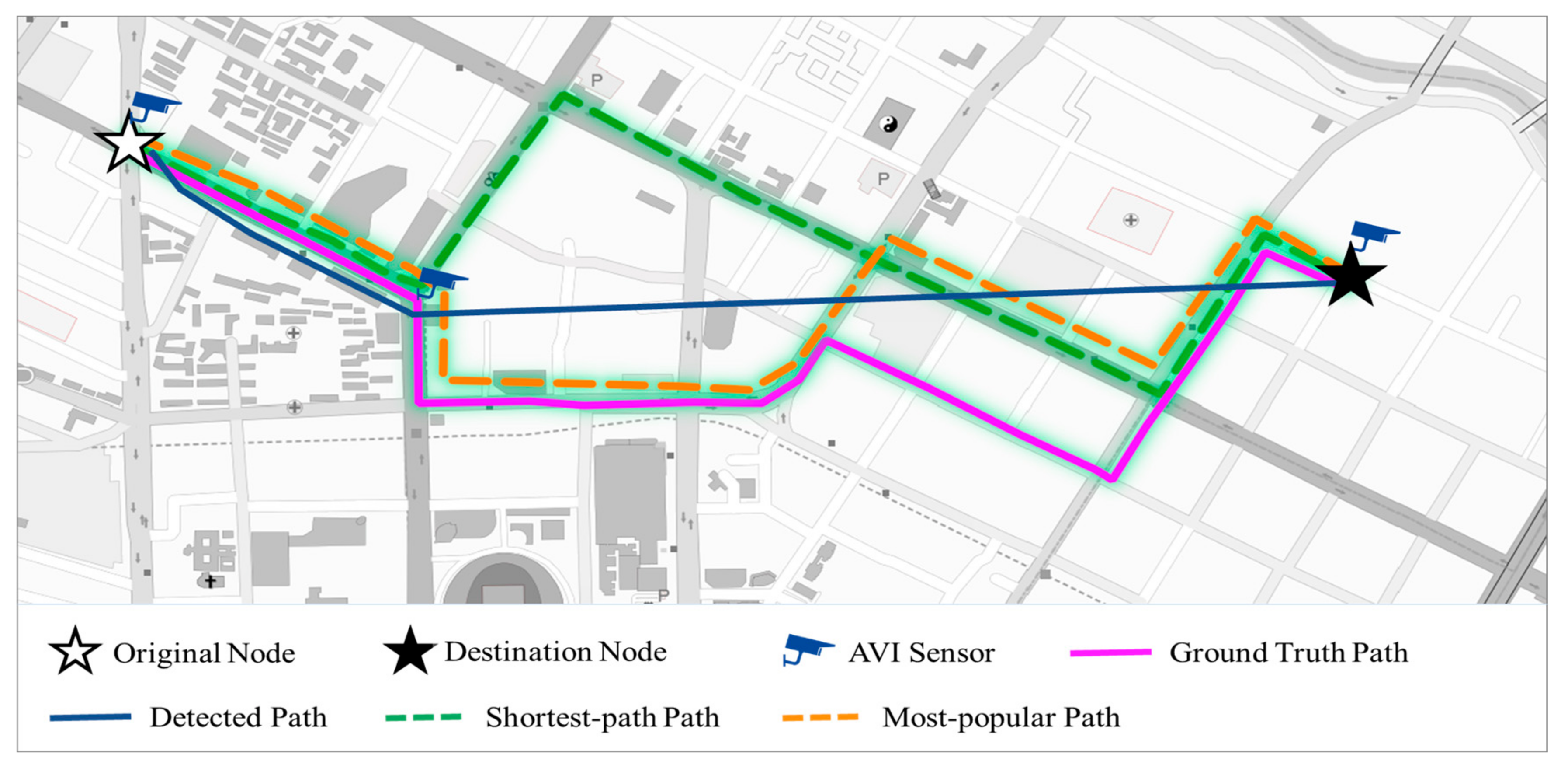
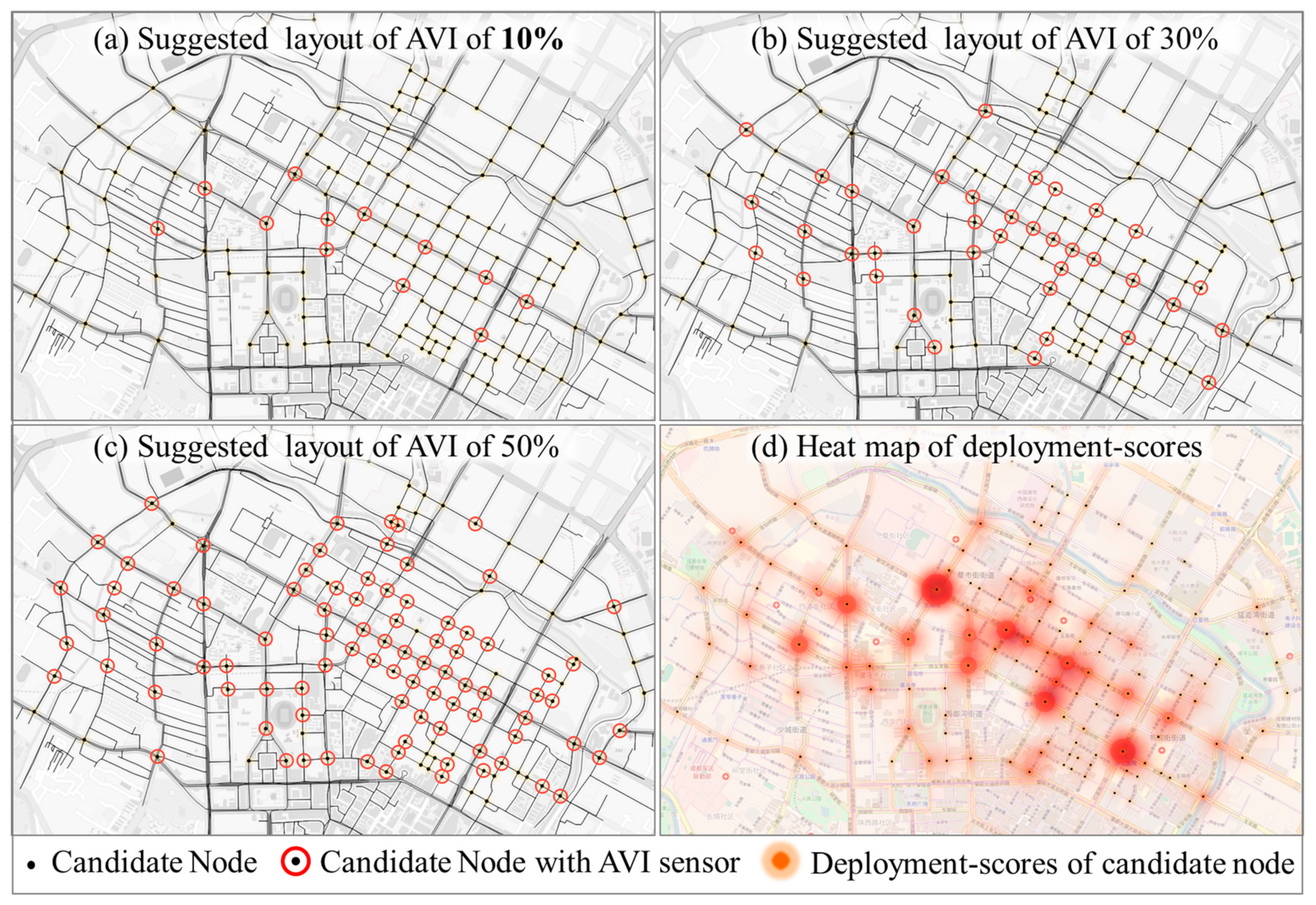
4.3. Experimental Results
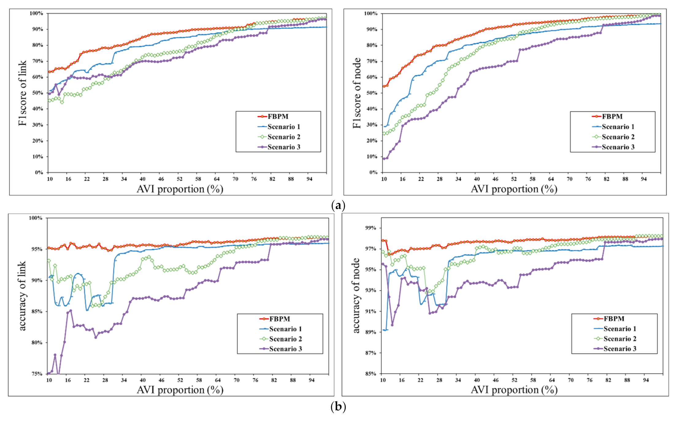
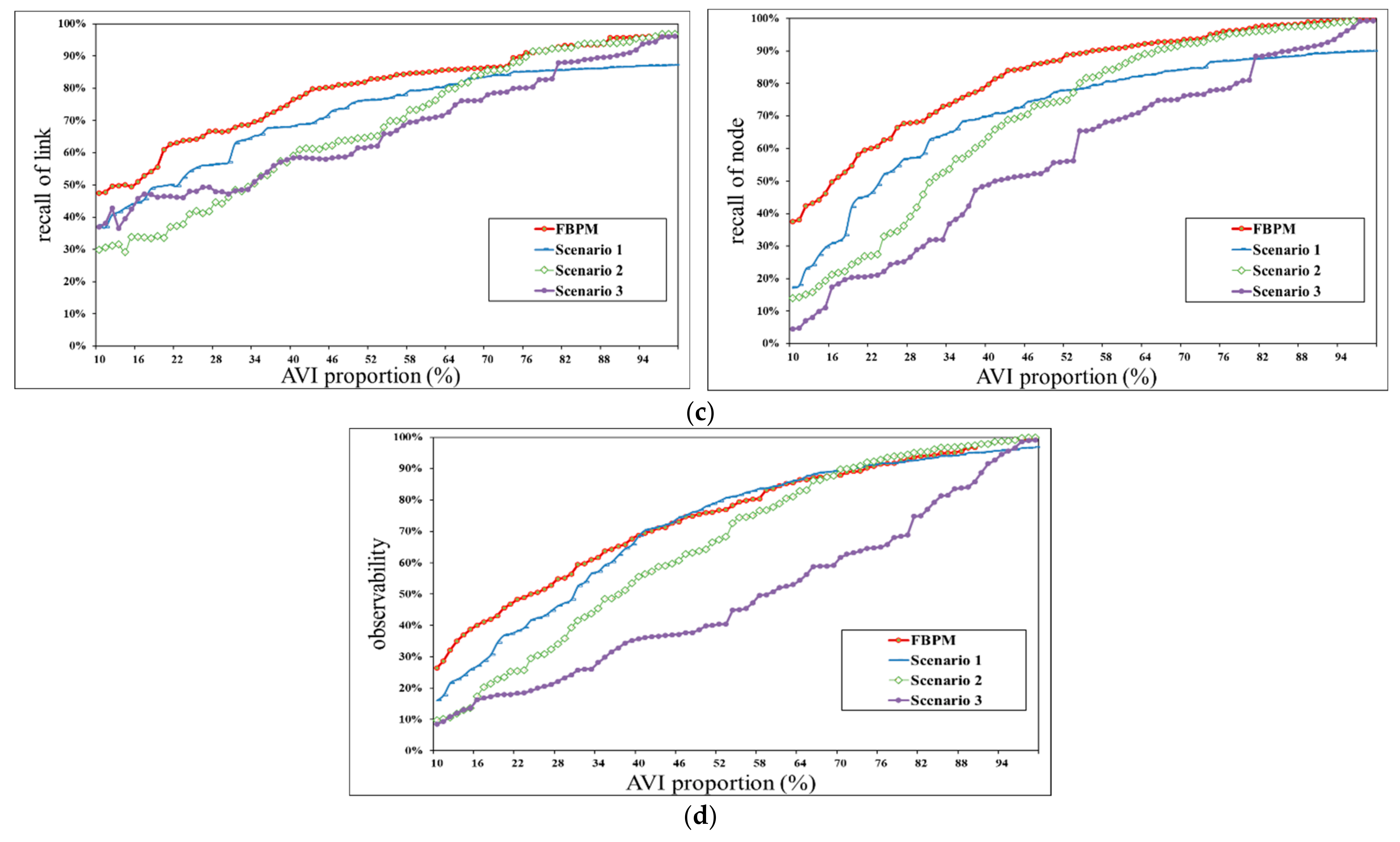
4.4. Comparative Experiments
5. Conclusions and Discussions
Author Contributions
Funding
Data Availability Statement
Conflicts of Interest
Disclosure Statement
Variables
| Variables | Details |
| Binary, equal to 1 if there is an AVI sensor established at node , and 0 otherwise | |
| Binary, equal to 1 if the path from i to j within path r is misidentified, and 0 otherwise | |
| Integer, the misidentified traffic flow from node i to node j of path r | |
| Integer, the total true traffic flow of path r | |
| Float, the misidentified length from node i to node j path r | |
| Float, the total length ofpath r | |
| C | The set of candidate nodes, C |
| L | The set of links between the candidate nodes |
| R | The set of the total actual vehicle paths; each path is represented as a sequence of candidate nodes that the vehicle passes |
| The set of the nodes in path r, |
References
- Fu, C.; Sayed, T. Random-Parameter Bayesian Hierarchical Extreme Value Modeling Approach with Heterogeneity in Means and Variances for Traffic Conflict–Based Crash Estimation. J. Transp. Eng. Part A Syst. 2022, 148, 04022056. [Google Scholar] [CrossRef]
- Mahmud, S.; Day, C.M. Leveraging Data-Driven Traffic Management in Smart Cities: Datasets for Highway Traffic Monitoring. In The Rise of Smart Cities; Butterworth-Heinemann: Oxford, UK, 2022; pp. 583–607. [Google Scholar] [CrossRef]
- Fu, C.; Sayed, T. Bayesian dynamic extreme value modeling for conflict-based real-time safety analysis. Anal. Methods Accid. Res. 2022, 34, 100204. [Google Scholar] [CrossRef]
- Castillo, E.; Grande, Z.; Calviño, A.; Szeto, W.Y.; Lo, H.K. A state-of-the-art review of the sensor location, flow observability, estimation, and prediction problems in traffic networks. J. Sens. 2015, 2015, 903563. [Google Scholar] [CrossRef] [Green Version]
- Sharma, S.K.; Phan, H.; Lee, J. An Application Study on Road Surface Monitoring Using DTW Based Image Processing and Ultrasonic Sensors. Appl. Sci. 2020, 10, 4490. [Google Scholar] [CrossRef]
- Jo, Y.; Ryu, S. Pothole Detection System Using a Black-box Camera. Sensors 2015, 15, 29316–29331. [Google Scholar] [CrossRef] [PubMed]
- Asad, M.H.; Khaliq, S.; Yousaf, M.H.; Ullah, M.O.; Ahmad, A. Pothole Detection Using Deep Learning: A Real-Time and AI-on-the-Edge Perspective. Adv. Civ. Eng. 2022, 2022, 1–13. [Google Scholar] [CrossRef]
- Cao, Q.; Ren, G.; Li, D.; Ma, J.; Li, H. Semi-supervised route choice modeling with sparse Automatic vehicle identification data. Transp. Res. Part C Emerg. Technol. 2020, 121, 102857. [Google Scholar] [CrossRef]
- Gentili, M.; Mirchandani, P.B. Locating sensors on traffic networks: Models, challenges and research opportunities. Transp. Res. part C Emerg. Technol. 2012, 24, 227–255. [Google Scholar] [CrossRef]
- Chen, H.; Chu, Z.; Sun, C. Sensor Deployment Strategy and Traffic Demand Estimation with Multisource Data. Sustainability 2021, 13, 13057. [Google Scholar] [CrossRef]
- Fu, H.; Lam, W.H.; Shao, H.; Kattan, L.; Salari, M. Optimization of multi-type traffic sensor locations for estimation of multi-period origin-destination demands with covariance effects. Transp. Res. Part E Logist. Transp. Rev. 2021, 157, 102555. [Google Scholar] [CrossRef]
- Owais, M.; Moussa, G.S.; Hussain, K.F. Sensor location model for O/D estimation: Multi-criteria meta-heuristics approach. Oper. Res. Perspect. 2019, 6, 100100. [Google Scholar] [CrossRef]
- Zhu, N.; Fu, C.; Zhang, X.; Ma, S. A network sensor location problem for link flow observability and estimation. Eur. J. Oper. Res. 2022, 300, 428–448. [Google Scholar] [CrossRef]
- Gentili, M.; Mirchandani, P.B. Review of optimal sensor location models for travel time estimation. Transp. Res. Part C Emerg. Technol. 2018, 90, 74–96. [Google Scholar] [CrossRef]
- Gentili, M.; Mirchandani, P.B. Locating Active Sensors on Traffic Networks. Ann. Oper. Res. 2005, 136, 229–257. [Google Scholar] [CrossRef]
- Mínguez, R.; Sánchez-Cambronero, S.; Castillo, E.; Jiménez, P. Optimal traffic plate scanning location for OD trip matrix and route estimation in road networks. Transp. Res. Part B Methodol. 2010, 44, 282–298. [Google Scholar] [CrossRef]
- Castillo, E.; Menéndez, J.M.; Jiménez, P. Trip matrix and path flow reconstruction and estimation based on plate scanning and link observations. Transp. Res. Part B Methodol. 2008, 42, 455–481. [Google Scholar] [CrossRef]
- Zangui, M.; Yin, Y.; Lawphongpanich, S. Sensor location problems in path-differentiated congestion pricing. Transp. Res. Part C Emerg. Technol. 2015, 55, 217–230. [Google Scholar] [CrossRef]
- Cerrone, C.; Cerulli, R.; Gentili, M. Vehicle-ID sensor location for route flow recognition: Models and algorithms. Eur. J. Oper. Res. 2015, 247, 618–629. [Google Scholar] [CrossRef]
- Fu, C.; Zhu, N.; Ling, S.; Ma, S.; Huang, Y. Heterogeneous sensor location model for path reconstruction. Transp. Res. Part B Methodol. 2016, 91, 77–97. [Google Scholar] [CrossRef]
- Ruiz, C.; Conejo, A.J. Pool Strategy of a Producer With Endogenous Formation of Locational Marginal Prices. IEEE Trans. Power Syst. 2009, 24, 1855–1866. [Google Scholar] [CrossRef]
- Salari, M.; Kattan, L.; Gentili, M. Optimal roadside units location for path flow reconstruction in a connected vehicle environment. Transp. Res. Part C Emerg. Technol. 2022, 138, 103625. [Google Scholar] [CrossRef]
- Bianco, L.; Confessore, G.; Gentili, M. Combinatorial aspects of the sensor location problem. Ann. Oper. Res. 2006, 144, 201–234. [Google Scholar] [CrossRef]
- Gendreau, M.; Laporte, G.; Séguin, R. Stochastic vehicle routing. Eur. J. Oper. Res. 1996, 88, 3–12. [Google Scholar] [CrossRef]
- Owen, S.H.; Daskin, M.S. Strategic facility location: A review. Eur. J. Oper. Res. 1998, 111, 423–447. [Google Scholar] [CrossRef]
- Alves, M.J.; Antunes, C.H. A new exact method for linear bilevel problems with multiple objective functions at the lower level. Eur. J. Oper. Res. 2022, 303, 312–327. [Google Scholar] [CrossRef]
- Torres, J.J.; Li, C.; Apap, R.M.; Grossmann, I.E. A Review on the Performance of Linear and Mixed Integer Two-Stage Stochastic Programming Software. Algorithms 2022, 15, 103. [Google Scholar] [CrossRef]
- van Slyke, R.M.; Wets, R. L-shaped linear programs with applications to optimal control and stochastic programming. SIAM J. Appl. Math. 1969, 17, 638–663. [Google Scholar] [CrossRef]
- Benders, J.F. Partitioning procedures for solving mixed-variables programming problems. Comput. Manag. Sci. 2005, 2, 3–19. [Google Scholar] [CrossRef]
- Rubin, P.; Gentili, M. An exact method for locating counting sensors in flow observability problems. Transp. Res. Part C Emerg. Technol. 2021, 123, 102855. [Google Scholar] [CrossRef]
- Freeman, L.C. A Set of Measures of Centrality Based on Betweenness. Sociometry 1977, 40, 35–41. [Google Scholar] [CrossRef]
- Wu, X.; Cao, W.; Wang, J.; Zhang, Y.; Yang, W.; Liu, Y. A spatial interaction incorporated betweenness centrality measure. PLoS ONE 2022, 17, e0268203. [Google Scholar] [CrossRef] [PubMed]
- Wang, X.; Niu, S.; Gao, J.; Zhang, J. A Study on the Highway Network Key Segments Identifying Method Based on the Structural Characteristics. CICTP 2014, 2014, 1819–1829. [Google Scholar] [CrossRef]
- Trolliet, T.; Cohen, N.; Giroire, F.; Hogie, L.; Pérennes, S. Interest Clustering Coefficient: A New Metric for Directed Networks Like Twitter. J. Complex Netw. 2021, 10, 597–609. [Google Scholar] [CrossRef]
- Xuebin, W. Optimizing Bus Stop Locations in Wuhan, China; University of Twente Faculty of Geo-Information and Earth Observation (ITC): Enschede, The Netherlands, 2010. [Google Scholar]
- Gurobi Optimization LLC. Gurobi Optimizer Reference Manual. 2018. Available online: https://www.gurobi.com/documentation/9.5/refman/index.html (accessed on 2 July 2022).


| Deployment Proportion of AVI Sensors | Link | Node | Observability | ||||
|---|---|---|---|---|---|---|---|
| 10% | 0.9521 | 0.4747 | 0.6335 | 0.9781 | 0.3753 | 0.5425 | 0.2638 |
| 20% | 0.9421 | 0.6092 | 0.7399 | 0.9697 | 0.5807 | 0.7264 | 0.4558 |
| 30% | 0.9485 | 0.668 | 0.7839 | 0.9712 | 0.6836 | 0.8024 | 0.5644 |
| 40% | 0.9572 | 0.7652 | 0.8505 | 0.9771 | 0.7979 | 0.8785 | 0.6878 |
| 50% | 0.9543 | 0.8164 | 0.88 | 0.9763 | 0.8693 | 0.9197 | 0.7599 |
| 60% | 0.9614 | 0.8483 | 0.9013 | 0.9788 | 0.9086 | 0.9424 | 0.8358 |
| 70% | 0.9632 | 0.8647 | 0.9113 | 0.9791 | 0.9347 | 0.9564 | 0.8788 |
| 80% | 0.967 | 0.9238 | 0.9449 | 0.9813 | 0.9695 | 0.9754 | 0.929 |
| 90% | 0.9679 | 0.9569 | 0.9624 | 0.9814 | 0.9893 | 0.9853 | 0.9685 |
Publisher’s Note: MDPI stays neutral with regard to jurisdictional claims in published maps and institutional affiliations. |
© 2022 by the authors. Licensee MDPI, Basel, Switzerland. This article is an open access article distributed under the terms and conditions of the Creative Commons Attribution (CC BY) license (https://creativecommons.org/licenses/by/4.0/).
Share and Cite
Li, D.; Wang, W.; Zhao, D. A Practical and Sustainable Approach to Determining the Deployment Priorities of Automatic Vehicle Identification Sensors. Sustainability 2022, 14, 9474. https://doi.org/10.3390/su14159474
Li D, Wang W, Zhao D. A Practical and Sustainable Approach to Determining the Deployment Priorities of Automatic Vehicle Identification Sensors. Sustainability. 2022; 14(15):9474. https://doi.org/10.3390/su14159474
Chicago/Turabian StyleLi, Dongya, Wei Wang, and De Zhao. 2022. "A Practical and Sustainable Approach to Determining the Deployment Priorities of Automatic Vehicle Identification Sensors" Sustainability 14, no. 15: 9474. https://doi.org/10.3390/su14159474