Heat Transfer Modeling on High-Temperature Charging and Discharging of Deep Borehole Heat Exchanger with Transient Strong Heat Flux

Abstract

High-temperature charging and discharging by deep borehole heat exchanger is typical of a large heat exchange temperature difference and transient strong heat flux. Simulation of this problem is not only computationally expensive, but it is also challenging in terms of robustness and stability for numerical methods. This paper formulates a generic and efficient heat transfer model with two distinctive novelties: Firstly, it highlights unsteady- and quasi-steady-state modeling strategies for heat transfer outside and inside a borehole. Secondly, this model provides analytical solutions for the heat front propagation and heat flux density distribution for unsteady-state heat transfer in the rock zone. These analytical formulations prove to be generic and critical to relieve computational effort in the face of strong heat flux. This model is validated by a typical high-temperature heat storage case from the literature, as well as the pilot demonstration project in China. It was discovered that a large prediction error of the heat transfer model only exists in very short operation days during the initial unsteady stages of charging and discharging. Both relative errors under charging and discharging phases are within 5% during the steady-state period. A comparison of the simulation cost with OpenGeoSys software demonstrates its high efficiency. It proves that this heat transfer model achieves an acceleration ratio of 30 times relative to the fully numerical method. In general, the heat transfer model has four advantages: generic applicability, good accuracy, easy implementation, and high efficiency, but it is limited to the heat transfer of a single deep borehole heat exchanger under pure heat conduction.

1. Introduction

Deep borehole heat exchanger shows great potential in large-scale heat storage in addition to geothermal energy extraction [1,2,3]. This offers great prospects for making full use of cross-seasonal surplus heat sources from abandoned solar energy or fluctuating district heating grids [4]. Thus, DBHEs have attracted increasing attention in recent years [5,6,7,8], especially in cold climate areas where heating load usually outweighs cooling [9,10] (Here, DBHE stands for deep borehole heat exchanger. All the abbreviations and notations mentioned in the paper are presented in Nomenclature). To obtain clear knowledge of the heat transfer characteristics of DBHE during the charging and discharging phases, prior heat transfer simulation is essential. However, high-temperature charging and discharging simulation of DBHE is typical of strong heat flux and intense heat transfer and is fundamentally distinctive from those widely studied single heat extraction scenarios. In general, it is rather challenging for traditional modeling approaches to handle this problem. A fully functional and easy-to-use heat transfer model with desired accuracy and great efficiency urgently needs to be developed.

The emerging critical issues in terms of the simulation of DBHE during high-temperature charging and discharging include, but are not limited to, the following:

(1) Current heat transfer models mainly center on the single heat extraction of DBHE. They can hardly depict the transient charging or discharging process of DBHE with strong heat flux around the borehole.

Extensive survey of the literature reveals that existing heat transfer models mainly focus on the heat transfer of DBHEs under single heat extraction conditions [11,12,13,14,15,16,17]. Although there are plenty of heat transfer models related to underground heat storage by BHEs or aquifers [18,19,20,21,22,23,24,25,26], most of them are limited to shallow BTES systems. A heat transfer model capable of simulating deep BTES has only been preliminarily studied [4,9,10]. To evaluate the heat storage potential of DBHE, Daniel carried out a few studies and developed a numerical simulator applicable for the thermal analysis of deep BTES [4]. However, in his simulations, the discharging temperature was not too high, reaching 30 °C, while the flow rate was quite small, at 14.4 m³/h. The simulation settings resulted in weak heat flux along the borehole depth and minor heat extraction output; thus, it is relatively not so challenging for simulation since extreme heat transfer would not occur in this scenario. Kristian and Bastian also investigated the heat storage performance of DBHE [9,10], but the dynamic charging and discharging process of a deep BTES system has not been fully illuminated, especially the transient evolution details of heat flux along the borehole depth at the initial unsteady charging or discharging stage. Large heat exchange temperature differences emerge during the high-temperature charging and subsequent discharging of actual deep BTES systems. Such a large heat exchange temperature difference undoubtedly leads to transient strong heat flux released into or extracted from the rock mass near the borehole. Therefore, the thermal performance of DBHE would evolve drastically throughout the whole operation. Despite the great efforts devoted to the heat transfer modeling of deep BTES systems [4,9,10], these models can only simulate DBHEs under near-constant heat extraction or a release rate with relatively weak heat flux. Existing methods can hardly handle this problem and are subject to temperature oscillation or even simulation failure [11]. It is imperative to develop heat transfer models that are applicable for actual deep BTES systems with strong heat flux.

(2) Current heat transfer models for DBHEs mainly focus on thermal response outside the borehole under the assumed charging or discharging load profile. They do not give full consideration to the tightly coupled interactions inside and outside the borehole.

In the modeling domain, a common practice to study the thermal response of a BHE assumes that it operates under a given load profile and uniform heat flux distribution, regardless of the coupled heat transfer inside and outside the borehole [27,28]. Many valuable studies have offered insightful conclusions about the thermal performance of shallow BHEs or DBHEs following this simulation idea. For example, Fang et al. formulated a novel algorithm for the thermal analysis of DBHE [11]. In their simulation, DBHE was assumed to operate under virtual heat extraction and release rates near 150 kW, while the heat flux was determined as approximately 75 W/m, which was uniform along the borehole depth. The manually assigned load profile does not necessarily match the actual heat extraction or heat release rate of DBHE, because both the heat extraction (or release) rate and heat flux dynamically evolve throughout the operation due to the transient rock temperature outside, and operational parameters (circulating flow rate and inlet temperature) inside the borehole. When it comes to heat flux along the borehole depth of DBHE, it is rather difficult to figure out a reasonable spatiotemporal distribution due to geothermal gradient and the operational parameters. More importantly, under the assigned load profile, it is impossible to discover the spatiotemporal evolution characteristics of heat flux during the unsteady charging and discharging stages. In essence, rock temperature outside the borehole and the real-time charging or discharging load of DBHE mutually affect each other. A thermal analysis for DBHE should fully consider the coupled heat transfer inside and outside the borehole. It is not reasonable to decouple the problem by assigning an improper load profile inside the borehole, which would even lead to simulation failure of DBHE, especially under the intense heat transfer conditions of charging and discharging concerned in this study.

(3). Current heat transfer models for DBHE have not properly balanced the simulation accuracy and computational cost.

A heat transfer analysis of DBHE can generally be carried out with either analytical or numerical methods [6,7,8,9,10,11,12,13,14,15,16,17]. Analytical modeling treats the borehole as an infinite or semi-infinite line heat source with constant heat flux [27,28]. Concise analytical solutions are available for the thermal response of rock due to heat release or the extraction of DBHE. In favor of its great advantage in rapid calculation, innovative analytical models and algorithms have been sought persistently by many researchers [13,14,15,16,17]. However, the analytical approach usually suffers from idealistic assumptions about a homogeneous medium with uniform initial temperature distribution. Moreover, analytical modeling may not be able to precisely handle the complex geological conditions and geothermal gradient effect in the deep subsurface, leading to oversimplification of the actual DBHE and poor simulation accuracy. This drawback has blocked its application in the thermal analysis of deep boreholes. In efforts to relieve the shortcomings of analytical modeling, different numerical models for the heat transfer of DBHE have also been presented over the past years [6,7,8,9,10,11,29,30,31,32,33]. Compared with the analytical approach, numerical models feature strong adaptability and flexibility. This approach can handle more realistic geological settings and follow strict boundary conditions without adopting simplified assumptions, as described above. Although numerical models could provide realistic simulation conditions and highly detailed physical parameters of the borefield, they may require enormous computation time [7,11,29]. This is because the numerical models for the heat transfer analysis of DBHE are usually based on fully discrete numerical schemes, which must deal with a great number of nodes/elements; for example, a DBHE array consisting of five boreholes studied with OpenGeoSys would need a total number of nodes and elements of 100,607 and 194,070, respectively [7]. Using a workstation equipped with a 2.20 GHz CPU and 64 GB of RAM, it took 143 h to accomplish a heating season simulation [7]. To achieve more efficient simulation of DBHE in GSHP and thermal energy storage systems, Zhang presented a new dimension reduction algorithm for heat transfer modeling of DBHEs cluster [29]. Comparisons with other commercial models and simulations on example cases showed that the computational efficiency can be improved by orders of magnitude. However, in their simulation, the heating load of DBHE was still assigned ideally, which did not consider the coupled heat transfer conditions inside and outside the borehole. Therefore, the simulation accuracy would be in doubt when employing this method for the transient charging and discharging simulation of deep BTES.

Transient simulation of the high-temperature charging and discharging of deep BTES with strong heat flux poses a great challenge for the robustness, stability, and simulation cost of traditional simulation methods. Up to now, no heat transfer models could simulate the extreme heat transfer problem with good accuracy, fast computation, and easy implementation. More importantly, the model setup is quite cumbersome, which would lead to extraordinarily high computational overhead. It is not good for wider applications. Additionally, there is still a lack of validation of the simulation results against an in situ field test. To address the problem, this paper presents a generic and efficient heat transfer model to perform comprehensive simulations of an actual deep BTES system consisting of a DBHE and high-temperature solar collector. It is applicable to both the charging and discharging process of DBHE with strong heat flux. This approach allows for tightly coupled interaction inside and outside the borehole during the transient heat transfer. Thus, the spatiotemporal evolution of heat flux density and the dynamic thermal performance of DBHE could be easily depicted. To our knowledge, it is the first time that heat flux density distribution along the borehole depth of DBHE under such an extreme heat transfer condition has been analytically revealed. This model is validated against a typical high-temperature heat storage case from the literature, as well as the in situ field test from a pilot demonstration project in China. Model validation proves that the dynamic heat transfer process of the deep BTES system could be captured with excellent accuracy. Moreover, the simulation cost demonstrates that this model is also highly efficient. Hence, many design aspects of the deep BTES system could be efficiently simulated and compared. The heat transfer model has four advantages: generic applicability, good accuracy, easy implementation, and high efficiency. It would also be promising for further optimization by integrating multiple operational parameters with the presented simulator.

2. Materials and Methods

In this section, a generic and efficient heat transfer model is developed for two separate phases including charging and discharging. In order to better illustrate the model development in this study, a generalized schematic is described in Figure 1. First, the basic design and operational parameters could be collected for model establishment, given the system configuration. Secondly, heat transfer modeling on the overall deep BTES system is formulated, including DBHE underground and high-temperature solar collector as the heat source during charging. Finally, the model is comprehensively validated in terms of simulation accuracy and simulation efficiency. There are two levels of coupling in the model. On one hand, it is the coupling within DBHE, i.e., heat transfer inside and outside of DBHE borehole is tightly coupled. On the other hand, it is the coupling between DBHE and the solar collector, i.e., DBHE is also coupled with the high-temperature solar collector.

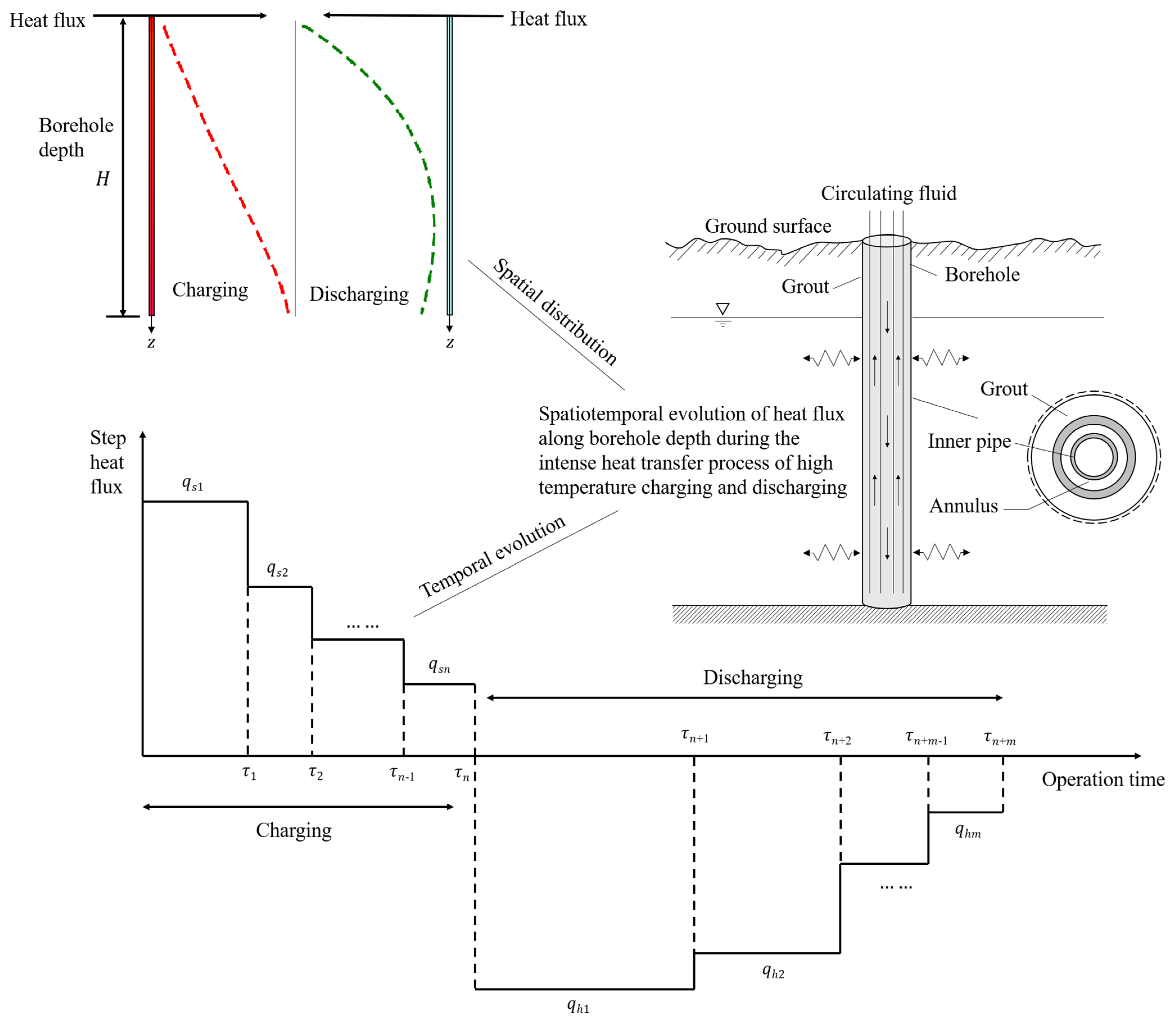
2.1. Transient Heat Transfer Model for DBHE

The transient thermal analysis of DBHE includes rock temperature distribution outside the borehole and variations of circulating water temperature in the inner and outer branches of the coaxial tube inside the borehole. In the rock zone, three-dimensional unsteady heat transfer occurs over a large range of time scales, depending on specific operation durations (short or long-term operation) [27]. It is coupled with the quasi-steady heat conduction within the borehole, as well as heat convection of the turbulent circulating fluid through complex boundary conditions [27]. In view of the transient characteristics of the high-temperature charging and discharging of DBHE, heat flux underground undergoes a dramatic evolution.

These transient heat fluxes lead to the rapid evolution of the rock temperature and high temperature gradient in the vicinity of the borehole. Figure 2 depicts the spatial and temporal distributions of the strong heat impulses. They are rather computationally demanding to capture during the dynamic heat transfer. We have proposed an efficient model for the thermal analysis of DBHE under heat extraction condition [15]. In this section, the original model is extended to be applicable for both charging and discharging simulations. This model highlights tight coupling between heat transfer inside and outside the borehole through heat flux density distribution at the interface. Firstly, with respect to unsteady heat transfer in the rock, analytical expressions for the heat front propagation and heat flux density distribution along the depth are schematically demonstrated. These analytical formulations are critical to relieving computational effort without resorting to local mesh refinement or demanding time step in the vicinity of the borehole where a high gradient of rock temperature exists. Secondly, as for quasi-steady heat transfer inside the borehole, both heat extraction and heat storage conditions of DBHE are formulated in detail.

2.1.1. Model Assumptions

In order to facilitate the heat transfer analysis, the following assumptions are taken into account in the model [15,28]: (1) Rock around the deep borehole heat exchanger is segmented layer by layer according to the vertical lithological stratifications along the depth. It is considered as a homogeneous medium whose thermo-physical parameters do not vary with temperature along the horizontal direction. (2). Rock outside the borehole is considered as a semi-infinite zone. Temperature fluctuation beneath the ground surface is ignored, and adiabatic boundary conditions are imposed at the top and bottom of the borehole, as well as the radial far field boundary. (3). Groundwater advection is neglected and heat transfer within the rock zone is simplified to be pure heat conduction.

2.1.2. Unsteady Heat Transfer Outside the Borehole

Ideally, heat conduction in the rock zone should be described as [27,28]:

$$\frac{1}{a_s}\frac{\partial T}{\partial \tau }=\frac{{\partial }^{2}T}{\partial r^2}+\frac{1}{r}\frac{\partial T}{\partial r}+\frac{{\partial }^{2}T}{\partial z^2}$$

(1)

where $a_s={\lambda }_s/{\rho }_s{c}_s$ denotes the rock thermal diffusion coefficient, while ${\lambda }_s$, ${\rho }_s$, and $c_s$ are the specific heat capacity, density, and thermal conductivity of rock, respectively.

Consider that the initial rock temperature varies near linearly along the depth (gradually increasing in accordance with the geothermal temperature gradient underground). In addition, radial heat flow dominates relative to that in the vertical direction [14,15]. Therefore, the vertical heat conduction term could be safely neglected, and the heat conduction equation could be further simplified as:

$$\frac{1}{a_s}\frac{\partial T}{\partial \tau }=\frac{{\partial }^{2}T}{\partial r^2}+\frac{1}{r}\frac{\partial T}{\partial r} \left(r_b<r<r_{\infty }\right)$$

(2)

where the borehole boundary is $r=r_b$, while $r=r_{\infty }$ represents the location of heat front propagation, which is also denoted as thermal affecting radius during heat transfer. Assuming that heat flux is injected into the rock domain at a certain rate near the borehole, satisfying the second type of boundary condition [14,15]:

$${-2\pi r_b{\lambda }_s\frac{\partial T}{\partial r}|}_{r=r_b}=q$$

(3)

The rock temperature field is fully developed near the heat front with no heat flux flowing in, satisfying [14,15]:

$${-2\pi r_{\infty }{\lambda }_s\frac{\partial T}{\partial r}|}_{r=r_{\infty }}=0$$

(4)

Therefore, heat conduction in the rock zone would be circumferentially homogeneous, i.e.,$T_s=T_s\left(r,z\right)$. Given the initial rock temperature profile$T_{init}\left(z\right)$along the depth, the solution to Equation (2) can be obtained by Laplace transformation, which determines the radial temperature distribution inside the heat front as [27]:

$$T_s\left(r,z\right)=T_{init}\left(z\right)-\frac{q}{2\pi {\lambda }_s}\frac{r_{\infty }^2}{\left(r_{\infty }^2-r_b^2\right)}\left[\ln \left(\frac{r}{r_{\infty }}\right)+\frac{1}{2}-\frac{1}{2}{\left(\frac{r}{r_{\infty }}\right)}^2\right]$$

(5)

Heat front outside the borehole would gradually propagate in the radial direction during the operation of DBHE. Evolution of the thermal affecting radius with operation time$\tau$reads as:

$$\frac{8a_s\tau }{r_b^2}=1+\frac{1}{{\left(r_b/r_{\infty }\right)}^2}+\frac{4}{1-{\left(r_b/r_{\infty }\right)}^2}\ln \left(\frac{r_b}{r_{\infty }}\right)$$

(6)

In view of the continuity constraints of rock temperature and heat flux at the interface of borehole, we have:

$$\{\begin{array}{l}{T}_s\left(r_b,\tau \right)=T_{init}\left(z\right)-\frac{q}{2\pi {\lambda }_s}\frac{r_{\infty }^2}{\left(r_{\infty }^2-r_b^2\right)}\left[\ln \left(\frac{r_b}{r_{\infty }}\right)+\frac{1}{2}-\frac{1}{2}{\left(\frac{r_b}{r_{\infty }}\right)}^2\right]\\ q=\frac{T_{f1}\left(z\right)-T_s\left(r_b,\tau \right)}{R_b}\end{array}$$

(7)

where $R_b$is the thermal resistance between the annulus of DBHE and the borehole wall.

Thereby, the solution for the radial heat flux density distribution along the borehole depth could be formulated as:

$$flu{x}_{radi}\left(z,\tau \right)=2\pi {\lambda }_s\frac{\left(r_{\infty }^2-r_b^2\right)\left(T_{init}\left(z\right)+\frac{Flux\left(z,\tau \right)}{\pi \left(r_{\infty }^2-r_b{}^2\right){\rho }_s{c}_s}-T_{f1}\left(z\right)\right)}{r_{\infty }^2\ln \frac{r_{\infty }^{}}{r_b}-\frac{1}{2}{r}_{\infty }^2+\frac{1}{2}{r}_b{}^2+2\pi {\lambda }_s{R}_b\left(r_{\infty }^2-r_b^2\right)}$$

(8)

where $Flux\left(z,\tau \right)$is the cumulative heat released into or extracted from the rock segment located radially in the vicinity of the borehole, and vertically at depth $z$ after an operation time of $\tau$. The physical formulation of heat flux distribution in Equation (8) is spatio-temporally resolved. It is determined by a combination of thermal affecting radius and initial rock temperature outside the borehole, as well as circulating water temperature inside the borehole. Moreover, this formulation could fully account for the rock stratification, because it is segmentally analytical over depth in essence.

The spatio-temporal formulation of heat flux distribution is especially beneficial to achieve efficient simulation with a large time step for the extreme heat transfer of high-temperature charging and discharging. Since it is an analytical solution, there is no stability issue when capturing the intense heat transfer, despite the high temperature gradient. Neither time-consuming iterations for the discretized heat conduction equations set nor mesh refinement are required for the simulation. More importantly, this formulation proves applicable to both the charging and discharging scenarios of DBHE, which are validated in the model evaluation section.

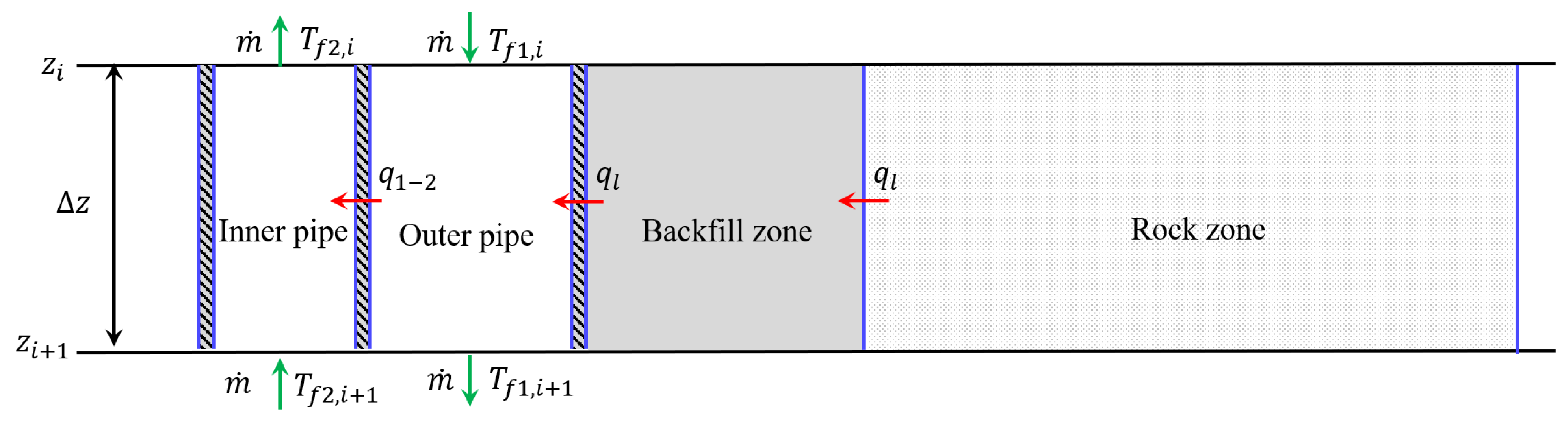
2.1.3. Quasi-Steady State Heat Transfer Inside the Borehole

This subsection performs a thermal analysis of the dynamic heat transfer within the borehole of DBHE operating under charging and discharging phases. As shown in Figure 3, flowing water could either be circulated downwards in the inner pipe and out of the annulus (heat storage mode) or downwards in the annulus of coaxial tube and out of the inner pipe (heat extraction mode). During the non-heating season, thermal energy carried by high-temperature water could be released continuously into the rock zone under the heat storage mode, while heat extraction mode is switched on by circulating low-temperature water through the annular space in full contact with the borehole wall during the heating season. Heat flux between the inner and outer branches of the coaxial tube contributed directly to the temperature variation of the circulating fluid. Therefore, the one-dimensional quasi-steady state heat transfer model could be adopted to establish the thermal balance relationship [27,28].

• Heat storage mode for charging phase

Under the heat storage mode, high-temperature circulating water outflows from the solar collector and is subsequently pumped into the inner pipe. As depicted in Figure 4, when the circulating water runs downward along the inner pipe, short-circuit heat flow exists due to the temperature difference between the inner pipe and annulus. This heat flow causes the circulating water to continuously cool down throughout the circulation. Then, as the circulating water runs upward along the annulus, it continues to be cooled until flowing out of the borehole. The temperature drop has two contributions: firstly, the short-circuit heat flow between the inner pipe and the annulus; secondly, the strong heat flux released into the rock elements on account of the large temperature difference relative to the borehole wall. With respect to the heat flux released into the rock zone, it is determined according to Equation (8), while the short-circuit heat flow between the inner pipe and annulus can be obtained based on the temperature difference of the circulating water and corresponding thermal resistance. Following the thermal balance relationship, it is easy to establish the quasi-steady state heat transfer model for heat storage mode as [15,28]:

$$\{\begin{array}{l}\dot{m}{c}_p\frac{\mathrm{d}{T}_{f1}\left(z\right)}{\mathrm{d}z}=\frac{T_{f1}\left(z\right)-T_{f2}\left(z\right)}{R_{12}}-flu{x}_{radi}\left(z,\tau \right)\\ \dot{m}{c}_p\frac{\mathrm{d}{T}_{f2}\left(z\right)}{\mathrm{d}z}=\frac{T_{f1}\left(z\right)-T_{f2}\left(z\right)}{R_{12}}\end{array}$$

(9)

Boundary conditions of the heat transfer problem read as:$z=0:T_{f1}\left(0\right)=t_{in}$; $z=H:T_{f1}\left(H\right)=T_{f2}\left(H\right)$. Where $\dot{m}$ and $c_p$ denote the circulating flow rate and specific heat capacity of the circulating water, respectively. $t_{in}$is the inlet temperature of the circulating water, $H$represents the drilling depth of the borehole, and $R_{12}$is the thermal resistance between the inner pipe and annulus. An iterative algorithm is applied to find the outlet temperature, as well as the fluid temperature distribution and heat flux density along the depth, given the inlet temperature and flow rate. The iteration stops until the heat flux density integral with the depth calculated as $Q_1={\displaystyle \sum }flu{x}_{radi}\left(z\right)\Delta z$balances with the heat loss determined by the temperature variation of the circulating water as $Q_2=c_p\dot{m}\left(t_{out}-t_{in}\right)$.

• Heat extraction mode for discharging phase

Similar to the thermal analysis of the heat storage mode, when DBHE operates under the heat extraction mode for discharging, the corresponding heat transfer described by Figure 5 could be modeled as following [15,28]:

$$\{\begin{array}{l}-\dot{m}{c}_p\frac{\mathrm{d}{T}_{f1}\left(z\right)}{\mathrm{d}z}=\frac{T_{f1}\left(z\right)-T_{f2}\left(z\right)}{R_{12}}-flu{x}_{radi}\left(z,\tau \right)\\ \dot{m}{c}_p\frac{\mathrm{d}{T}_{f2}\left(z\right)}{\mathrm{d}z}=\frac{T_{f2}\left(z\right)-T_{f1}\left(z\right)}{R_{12}}\end{array}$$

(10)

The numerical solutions for Equations (9) and (10) are all based on second order central difference schemes, and the discretized finite difference equations are not formulated for simplicity.

2.2. High-Temperature Solar Collector Model

The high-temperature circulating water for charging DBHE is supplied by a solar collector in the summer season. Figure 6 presents the flat-plate solar collector coupled with the DBHE underground. It has a simple structure and good thermal performance with a low cost, which could meet the general heating load of high-temperature circulating water reinjected into the DBHE underground. The classical Hottel–Whillier steady-state model is applied to describe heat transfer within the solar collector as [34]:

$$Q_u=I_c{A}_c{F}_R\left[{\left(\tau \alpha \right)}_e-\frac{U_l\left(t_{ci}-t_a\right)}{I_c}\right]$$

(11)

where $Q_u$ is the real-time solar energy collected by the solar collector, W; $I_c$ denotes the solar radiation intensity, W/m²; $A_c$ stands for the collector area, m²; $F_R$is the heat migration factor; ${\left(\tau \alpha \right)}_e$represents the product of effective transmission ratio and absorption ratio; $U_l$is the heat loss coefficient, W/(m²∙°C); and $t_{ci}$ and$t_a$are the inlet water temperature and outdoor air temperature, respectively, °C.

On the circulating flow side of the collector, we have:

$$Q_u=c_p\dot{m}\left(t_{co}-t_{ci}\right)$$

(12)

where $t_{co}$is the outlet temperature of circulating flow, °C.

Combining Equations (11) and (12), the inlet flow temperature returning into DBHE could be determined as:

$$t_{co}=\left(1-\frac{A_c{F}_R{U}_l}{c_p\dot{m}}\right)t_{ci}+\frac{A_c{F}_R{I}_c{\left(\tau \alpha \right)}_e}{c_p\dot{m}}+\frac{A_c{F}_R{U}_l}{c_p\dot{m}}{t}_a$$

(13)

The overall heat transfer simulation procedure of the deep BTES system under charging or discharging phases can be summarized in Figure 7. This flow chart acts as the guideline for all the simulation results in the case study performed in Section 3.

3. Results

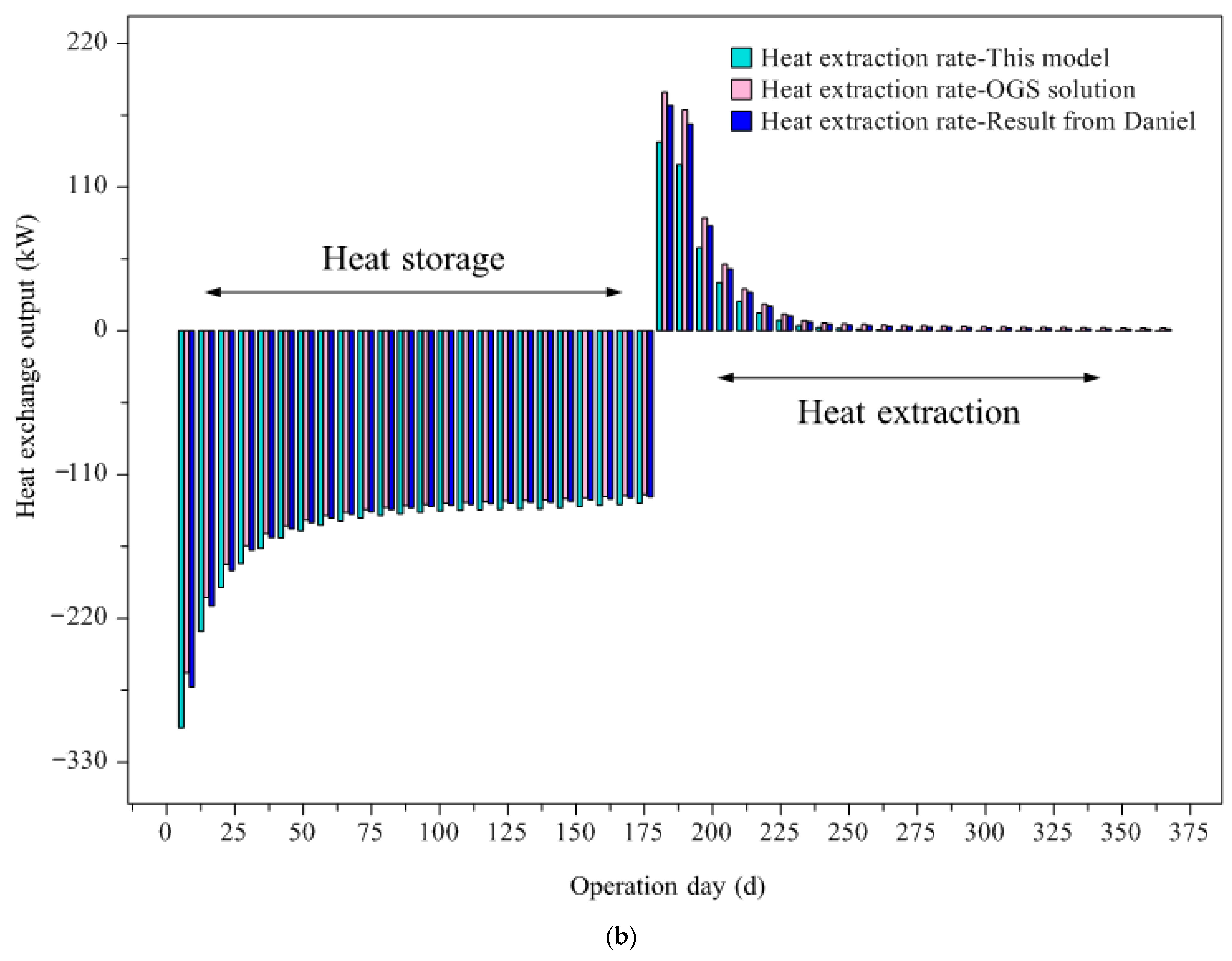
3.1. Model Validation Based on a Typical High-Temperature Heat Storage Case from the Literature

This subsection performs cross validation of the heat transfer model on the basis of a typical high-temperature heat storage case by DBHE from the literature. This deep BTES case is located at the Technical University of Darmstadt, Germany [4]. Its model parameters are shown in

Table 1. Model parameters for the deep BTES case.

Geological Parameters		Borehole Heat Exchanger Parameters
Parameter	Value	Parameter	Value
Thermal conductivity of rock	2.6 W/m/K	Borehole radius	152.2 mm
Bulk heat capacity of rock	2.3 MJ/m3/K	Inner diameter of annulus	127 mm
Thermal conductivity of geofluid	0.65 W/m/K	Annulus wall thickness	5.6 mm
Bulk heat capacity of geofluid	4.2 MJ/m3/K	Inner diameter of inner pipe	75 mm
Porosity of rock	0.01	Inner pipe wall thickness	6.8 mm
Subsurface temperature	10 °C	Thermal conductivity of annulus (steel pipe)	54 W/m/K
Geothermal temperature gradient	30 °C/km	Thermal conductivity of inner pipe (PE pipe)	0.4 W/m/K
Permeability coefficient	10−8 m/s	Thermal conductivity of backfill	2 W/m/K
Hydraulic gradient in the rock	0	Bulk heat capacity of heat carrier (water)	4.12 MJ/m3/K
Model length	400 m	Thermal conductivity of heat carrier (water)	0.65 W/m/K
Model width	400 m	Dynamic viscosity coefficient of heat carrier (water)	5.04 × 10−4 kg/m/s
Model depth	2000 m	Density of heat carrier (water)	977 kg/m3

. The total operation time of the case lasted for a year, of which the first six months were designed for heat storage, and the following 6 months for heat extraction. The alternating operation of heat storage and extraction was achieved by varying the inlet temperature of circulating water. In view of the heating capacity of the solar collector and thermal resistant limit of the inner pipe installed in the coaxial DBHE, the inlet temperature of the circulating water was controlled at 90 °C to store heat underground during the non-heating season. The return water temperature was set as 30 °C during the heat extraction phase, in order to heat the building terminal in direct supply mode without heat pump units. During operation, the volumetric flow rate of the circulating water through DBHE was set constant to be 14.4 m³/h. It was determined based on a combined optimization of the heat exchange capacity of deep BTES and energy consumption of the circulating pumps to achieve efficient heat storage and supply.

The cross validation of the heat transfer model for deep BTES was performed against the literature data and simulation results from OGS software. Figure 8 compared the thermal performance of a single DBHE over a complete operation cycle. Two key thermal performance parameters of DBHE including real-time outlet temperature and heat exchange rate are fully validated against each other throughout the charging and discharging phases. From the evolution curves during operation, it is easy to see that the simulation results of the model agree well with the OGS solutions and the literature data. Minor deviation only exists in the initial unsteady state phase (around 10 days) of heat storage or extraction. The unsteady state stage in this case lasts for about 10 days (heat storage or heat extraction) and accounts for only 5% of the overall operation time. It can be confirmed that the simulation accuracy of the proposed model for the heat transfer of DBHE under high-temperature charging and discharging has a high degree of credibility. In addition, due to the high inlet temperature of returning water into DBHE, there is almost no heat exchange temperature difference at the late stage of discharging. Therefore, the heat extraction output is eventually close to zero.

3.1.1. Simulation Accuracy of the Model

Table 2. Comparison of key thermal performance indicators during the operation of deep BTES.

	Literature Data	OGS Solution	Result of This Model
Total heat storage (MWh)	665.68	653.16	701.48
Total heat extraction (MWh)	103.33	112.88	78.17
Average heat storage rate (kW)	152.4	149.53	160.6
Average heat extraction rate (kW)	23.65	25.84	17.89
Average heat flux density during charging (W/m)	76.2	74.77	80.3
Average heat flux density during discharging (W/m)	11.83	12.92	8.95
Heat storage efficiency	15.52%	17.28%	11.14%

gives a detailed comparison of the overall thermal performance indicators of deep BTES over the entire charging and discharging phases, including total heat storage amount, average heat storage rate, and average heat flux density. The statistical results show that there is little difference between the literature data, OGS software, and our model during charging phase. The average heat flux density along the borehole depth is 76.2 W/m, according to the literature data, while the OGS solution is 74.77 W/m with a relative error of 1.88%, and the simulation result of the model is 80.3 W/m with a relative error of 5.38%. However, during the discharging period, the results of the three predictions show considerable distinction. According to the literature data, the average heat flux density value is 11.83 W/m. The OGS solution is 12.92 W/m, which gives a prediction error of 9.21% relative to the original literature data. The simulation result from this model is 8.95 W/m, and its prediction error amounts to 24.34%. In view of the large deviation in the heat extraction output of the three predictions during the discharging phase, there is also a significant difference in the heat storage efficiency. The reference results (OGS solution and literature data) are 15.52% and 17.28%, respectively, while the simulation result of this model is lower at 11.14%. Since the heat extraction rate decreased rapidly at the initial start-up due to a large temperature difference, it requires demanding time resolution. However, this model adopts quite a large time step to achieve computational efficiency. Thus, the heat extraction rate recorded that every time step would be smaller than the time averaged result, leading to a larger prediction error.

The large deviations also originate from the comparison scheme in Table 2, which is based on the heat exchange amount rather than the outlet temperature. Given the operation condition (inlet water temperature, flow rate) and geological settings for deep BTES, only outlet temperature is the basic thermal performance parameter. Outlet temperature directly reflects the simulation accuracy. However, the heat exchange rate during operation is based on the outlet and inlet temperature difference, and inaccuracy of the outlet temperature predicted by the heat transfer model or OGS solution would be amplified when calculating the heat exchange rate.

Moreover, it can be found that large deviations mainly exist at the unsteady stage in Figure 8a. In order to further validate the accuracy of the heat transfer model, the simulation results of the outlet temperature at the unsteady state stage during charging and discharging are compared and analyzed subsequently (see

Table 3. Comparison of outlet temperature during the unsteady stage of charging and discharging phases for the typical high-temperature storage case.

	Literature Data	OGS Solution	Result of This Model
Average outlet temperature during charging (°C)	71.03	71.85	68.7
Average outlet temperature during discharging (°C)	44.45	45.31	41.99
Relative error during charging	-	1.15%	3.28%
Relative error during discharging	-	1.93%	5.53%

). At the unsteady stage under heat storage condition, the predicted outlet temperatures are 71.03 °C from the literature data, 71.85 °C for the OGS solution with a relative error of 1.15%, and 68.7 °C for the model in the study with a relative error of 3.28%. The corresponding temperature difference of circulating water and heat storage rate are 18.97 °C/318.69 kW, 18.15 °C/304.92 kW and 21.3 °C/357.84 kW, respectively. In contrast, as for the unsteady state stage under heat extraction condition, the average outlet temperature is 44.45 °C according to the literature data, while the OGS solution is 45.31 °C with a relative error of 1.93%, and the prediction of the model is 41.99 °C with a relative error of 5.53%. The temperature difference of circulating water and the heat extraction rate are accordingly valued at 14.45 °C/242.76 kW, 15.31 °C/257.21 kW and 11.99 °C/201.43 kW. It is discovered that the prediction errors at the unsteady stage of charging and discharging phases are all around 5%, which basically satisfies the accuracy requirement of the engineering application.

3.1.2. Simulation Efficiency of the Model

Due to the analytical solutions for the thermal affecting radius and heat flux distribution along the borehole depth, the time step for the charging or discharging of DBHE could be set large enough, which is even comparable to the running hours for the operation condition. This case study was carried out on a common computer with the CPU of 2.9 GHz and RAM of 16 GB. According to our simulation, dynamic heat transfer of the deep BTES system evolves with the time step every 12 h, whereas the traditional numerical approach should be limited to a time step of several minutes or seconds if the explicit numerical scheme is adopted. During the 180 days of charging and 185 days of discharging, the simulation costs for the overall cycle of deep BTES based on our efficient model versus the fully numerical approach by OGS software 6.4.2 (Helmholtz Centre for Environmental Research-UFZ, Leipzig, Germany), are shown in

Table 4. Comparison of simulation cost between OGS software and this model.

Simulation Cost	OGS Software	This Model
Simulation for charging phase	7.51 h	0.25 h
Simulation for discharging phase	7.7 h	0.26 h

. Compared to the traditional numerical method by OGS, the model is highly efficient. Simulation for both the charging and discharging phases of the deep BTES system demonstrates that our efficient heat transfer model achieves an acceleration ratio of 30 times, approximately. With respect to the charging simulation, 7.51 h was needed for the fully numerical method by OGS, while it only took around 15 min (0.25 h) by our model. Moreover, as discussed above, the simulation results provided by the model are also in good agreement with the OGS solution. It indicates that the heat transfer model to perform the thermal analysis of the deep BTES system is both reasonable and efficient for the design or optimization of a practical project.

3.2. Model Validation against In Situ Field Test of a Demonstration Project

This section continues model validation against an in situ field test of a pilot demonstration project under operation.

3.2.1. Project Overview

The pilot demonstration project of a ground source heat pump system with DBHE for the thermal performance analysis of deep BTES in this paper is located in Qingdao, China [15]. This project is designed for residential heating. The building floor area is roughly estimated as 24,000 m² with the heating demand of 50 W/m², and the total heating load sums up to be 1200 kW. During the operation for heating, it is expected to provide a maximum water supply temperature of 50 °C for the building terminal. According to the geothermal exploration data (including geothermal temperature gradient, rock layers and fracture development underground, etc.) in Qingdao area, it shows that the average geothermal temperature gradient of the borehole is 2.8 °C/100 m, which is lower than the expected 3 °C/100 m. In view of the geothermal condition, the coaxial heat exchanger is installed in the deep borehole with a total depth of 2600 m and a borehole diameter of 216 mm. The temperature of the surrounding rock layer is about 85 °C at the bottom of the borehole. The deep borehole heat exchanger takes water as a heat carrier, and its detailed design parameters are summarized in

Table 5. Geological parameters of the deep borehole.

Parameter	Value
Surface temperature (°C)	15
Geothermal temperature gradient (°C/km)	28
Lithological stratifications	5
Groundwater conditions	Without ground water advection

,

Table 6. Thermophysical properties of rock layers.

Rock Layers	Rock Type	Depth (m)	Thermal Conductivity (W/m/K)	Specific Heat Capacity (J/kg/K)	Density (kg/m3)
Layer 1	Soil	0~100	1.16	840	1500
Layer 2	Basalt	100~1985	2.78	925	2800
Layer 3	Sandstone	1985~2410	2.8	920	2800
Layer 4	Limestone	2410~2470	2.75	900	2780
Layer 5	Sandstone	2470~2600	2.8	920	2800

and

Table 7. Design parameters of the deep BTES.

Design Parameters	Value
Drilling depth of DBHE (m)	2600
Inner pipe diameter of DBHE (mm)	90/110
Outer pipe diameter of DBHE (mm)	159/178
Borehole diameter of DBHE (mm)	216
Solar collector area (m2)	25

.

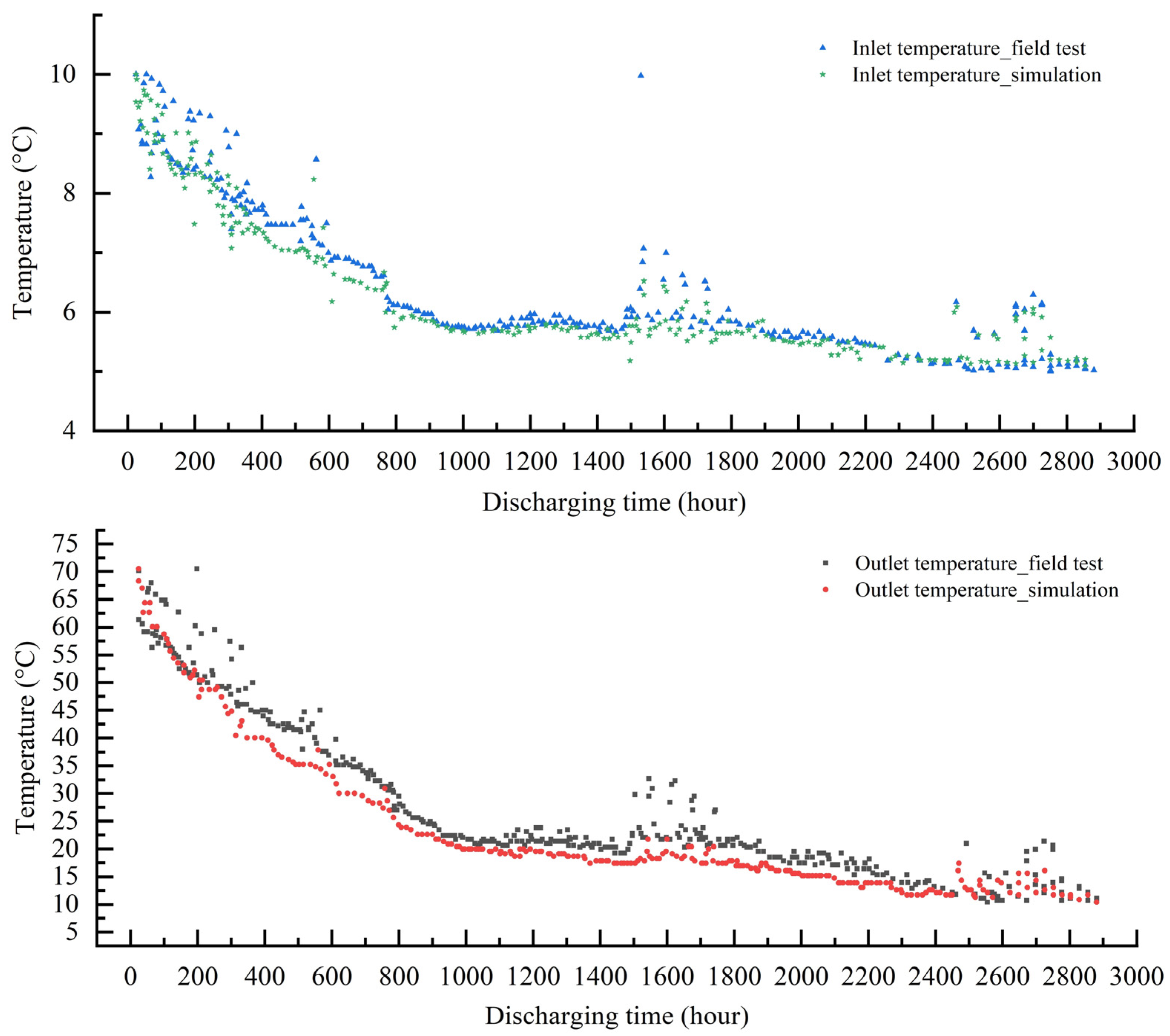
3.2.2. In Situ Field Test of the Project under Operation

The project started commissioning on 19 September 2016. It was officially put into heat storage on 23 September 2016 and ceased operation on 22 October 2016, with a total charging period of 30 days prior to discharging for heat supply. After ten days of intermittence, it went on operating for heat supply from 1 November 2016 to 1 March 2017 and discharged for 120 days during the heating season. To validate and further calibrate the heat transfer model of DBHE, this subsection focuses on the in situ field test data from the real-time operation of the project as reference for the deep BTES system. The operational parameters of the ground source heat pump system with DBHE were collected on site, including inlet and outlet temperature, as well as the flow rate of the circulating water on the ground source side. All the temperature data are acquired from the online control system of deep BTES every 5 min with a measurement error of −0.3 to +0.3 °C. As for the circulating flow rates, they are measured based on portable ultrasonic flow meters (THF-2000P) with an accuracy of ±1.0%, which are installed on the return side into DBHE. The hourly heat exchange power on the ground source side was based on heat meters, including heat storage and heat extraction rate. During the test period, the deep BTES system operated with a constant flow rate. The heat pump units shut down during the charging phase but switched on during the discharging phase. The operational parameters for the deep BTES during the charging and discharging phases are summarized in

Table 8. Operational parameters for the deep BTES during charging and discharging.

Operational Parameters	Value
Charging time (days)	30
Discharging time (days)	120
Flow rate during charging (m3/h)	20
Flow rate during discharging (m3/h)	50
Solar radiation intensity (W/m2)	550~850
Operation hours per day (hour)	24

.

Figure 9 shows the results of the thermal response of DBHE under the charging condition, where the inlet temperature returning from the solar collector ranged within 95~110 °C, according to Equation (13) and fluctuation of the solar radiation intensity. It could be clearly seen that a good agreement between the field test and simulation of the model was achieved. The outlet temperature rose gradually with operating time due to the continuous release of heat flow into rock from the high-temperature water circulating into DBHE. However, there is a larger difference of the model prediction result, relative to the field test, which is especially noticeable during 200~280 h of the charging time, and the model gives a comparatively lower estimation of the outlet temperature over the field test. This originates from underestimation of effective operation time ${\tau }_{eff}$ according to our finding. Theoretically, ${\tau }_{eff}$proves longer than real operation hour$\tau$at the initial operation period of DBHE, since shorter operation time corresponds to the smaller thermal affecting radius from Equation (6), and smaller thermal affecting radius results in larger heat flux density released into rock, as indicated by Equation (8). Therefore, as high-temperature water circulates through DBHE, it cools down more rapidly than real-time temperature. Despite the local error of the outlet temperature in the initial charging days, a close agreement can still be observed in Figure 9. As expected, the outlet temperature soon reached a relatively steady state due to continuous charging. Moreover, the model prediction result is nearly the same as the field test towards the steady state. Thus, the dynamic heat transfer model for the thermal performance evaluation of deep BTES under heat storage condition was well validated.

The thermal performance of DBHE during the discharging period after heat storage is presented in Figure 10. As the heating demand of the building terminal gradually increased, the inlet temperature of DBHE was lowered properly from 10 °C to 5 °C to obtain a larger heat extraction output underground. Similar to the charging condition, the temperature difference between the outlet and inlet circulating water decreased quickly with operation time at the beginning of discharging, owing to continuous heat extraction from rock. Then, it gradually decreased after 1400 h, and finally remained almost steady at 15/5 °C, respectively. Moreover, a lower outlet temperature of DBHE could be observed during discharging in comparison with field test data, as depicted in Figure 10. Similar to the thermal analysis of heat front propagation discussed during the charging phase, this model tends to give a smaller estimation of the thermal affecting radius. Thus, the rock temperature near the borehole would drop even more on account of the cumulative heat extraction amount, according to Equation (14) as following:

$$\Delta t\left(z,\tau \right)=\frac{{\displaystyle \sum _{\tau }flux\left(z,\tau \right)}}{\pi \left(r_{\infty }^2-r_b{}^2\right){\rho }_s{c}_s}$$

(14)

Consequently, it results in a smaller heat exchange temperature difference between the borehole and circulating water, as well as a lower outlet temperature. Perfect agreement between the simulation results and in situ field test is also achieved during the discharging phase, which once again demonstrates the credibility of the heat transfer model for the deep BTES system proposed in this study.

3.2.3. Model Validation during Charging

During the charging phase, rock near the borehole was heated close to 100 °C, which is in approximate equilibrium with the high-temperature circulating water. According to our numerical simulation, at the top section of the borehole, the temperature difference between circulating water and the surrounding rock could be up to 56 °C during the initial stage of charging. In contrast, the inlet temperature of circulating water was lowered to 5 °C during discharging. The heat exchange temperature difference could reach as high as approximately 85 °C at the initial start-up. In comparison with the typical high-temperature heat storage case discussed above, there was strong local heat flux around the borehole. Simulation of this problem poses a great challenge for the robustness and stability of traditional numerical methods such as the finite element or finite difference methods, because numerical methods often require local mesh refinement near the borehole wall and a demanding time step to cope with this tough problem. Only the grid with sufficient spatio-temporal resolution could capture the rapid evolution of the rock temperature field, as well as details of the transient heat transfer.

Despite the great challenge in the face of transient strong heat flux, this model is quite robust and does not lead to oscillation or failure of the charging and discharging simulations. To demonstrate the simulation accuracy and efficiency, we continue to cross validate the simulation results of the key thermal performance indicators of deep BTES in this section. Figure 11 presents the dynamic evolution of heat flux density and circulating water temperature along the borehole depth over the charging phase. Overall, the model prediction remains consistent with the OGS solution. It successfully captures the trend of charging heat flux density decreasing with operation time.

Table 9. Comparison of average heat flux density along depth during charging.

Charging Time (day)	OGS Solution (W/m)	Result of This Model (W/m)	Relative Error
			Average Error	Maximum Error
5	242.16	253.94	4.61%	13.72%
10	182.02	188.49	3.65%	8.71%
15	179.19	183.32	2.72%	4.13%
20	135.04	136.55	1.81%	4.36%
25	120.18	121.56	1.8%	4.35%
30	111.0	113.47	2.75%	4.78%

compares the average heat flux density clearly, which was 253.94 W/m at 5 days. After a rapid decline, it drops to 113.47 W/m at the end of charging. The prediction error for the average heat flux density was within 5% between the OGS solution and this model.

The maximum error of heat flux density was 13.72% at the initial charging and 4.78% at the end. It was also observed that the maximum error was located at the top section of the borehole during the initial charging from 5 to 15 days, and it moved toward the bottom from 20 to 30 days. Evolution of circulating water temperature in DBHE achieved an excellent agreement between the model and OGS solution, as clearly depicted in Figure 11. During the initial unsteady charging stage, the model predicted an average outlet temperature of 73.72 °C at 5 days, with a relative error of 0.89% against the OGS solution (74.38 °C). At the steady stage, the average outlet temperature reached 84.51 °C according to the OGS solution, while the model prediction was 84.07 °C with an error of only 0.52%. To further validate this model, a comparison of the simulation results against the field test was summarized in

Table 10. Comparison of outlet temperature during the unsteady stage of charging and discharging phases.

	Field Test	OGS Solution	Result of This Model
Average outlet temperature during charging (°C)	69.29	74.38	73.72
Average outlet temperature during discharging (°C)	48.35	41.35	39.64
Relative error during charging	-	7.34%	6.39%
Relative error during discharging	-	14.47%	18.01%

and

Table 11. Comparison of outlet temperature during the steady stage of charging and discharging phases.

	Field Test	OGS Solution	Result of This Model
Average outlet temperature during charging (°C)	79.31	84.51	84.07
Average outlet temperature during discharging (°C)	10.75	10.77	10.70
Relative error during charging	-	6.55%	6%
Relative error during discharging	-	0.18%	0.46%

. Depending on the real-time solar radiation collected by the solar collector during the in situ field test, the inlet temperature returning into DBHE may fluctuate. However, it was kept constant at 100 °C in simulation by this model and OGS software. Therefore, the comparison error is rather noticeable. However, it was still not more than 10%, which valued at 6.39% during the unsteady charging stage and 6% at the steady stage. Consequently, the simulation credibility of the model was confirmed.

3.2.4. Model Validation during Discharging

Similar to the thermal analysis for deep BTES during the charging phase, we continued to compare the simulation results when the operation arrived at the discharging period. The dynamic evolution of the heat flux density and circulating water temperature along the borehole depth over the discharging phase is depicted in Figure 12. It shows that the maximum temperature of the borehole wall after heat storage could reach 85 °C (at the top section of borehole). When the return water temperature was set at 5 °C, the temperature difference inside and outside of the borehole could be up to 80 °C. Under such a large heat exchange temperature difference, the average heat flux density along the borehole depth was as high as 1500 W/m at the initial discharging, and the maximum local heat flux density could even reach 3000 W/m. An extremely refined spatio-temporal resolution is required to capture the intense heat transfer at the unsteady stage, and the simulation results are quite sensitive to the advancing time step. Despite this challenge, this model still succeeded in simulating the dynamic heat flux density, which evolved even more drastically underground.

Table 12. Comparison of average heat flux density along depth during discharging.

Discharging Time (day)	OGS Solution (W/m)	Result of This Model (W/m)	Relative Error
			Average Error	Maximum Error
1	1549.45	1476.25	4.38%	12.07%
5	1163.24	1115.03	4.13%	12.06%
10	720.26	689.81	4.38%	12%
20	511.98	490.5	4.38%	12.02%
30	226.34	217.08	4.05%	9.78%
40	169.73	162.89	3.73%	7.68%
50	149.46	142.63	4.21%	8.23%
120	116.55	118.36	1.88%	3.52%

compares the simulation results of average heat flux density between OGS and this model. The transient strong heat flux density was as high as 1476.25 W/m at 1 day and rapidly decreased to 1115.03 W/m at 5 days with a reduction of 24.46%. Subsequently, it continued to drop, with a density of 490.5 W/m at 20 days, until finally dropping to 118.36 W/m at the end of the discharging, which was only 8.02% of the initial heat extraction output. Similar to the charging condition, the prediction error of the average heat flux density was also within 5%. The maximum prediction error was approximately 12% at the unsteady stage and 3.52% at the end. In addition, the maximum error was also located at the top section of the borehole within 5 days of the initial discharging stage. However, a larger prediction error occurred at both the top and bottom during a transition period from 5 to 20 days. Then, it gradually shifted to the bottom from 20 days to 120 days. During the initial unsteady discharging stage, the average outlet temperature was 48.35 °C based on the field test, while the OGS software and this model predicted the outlet temperatures as 41.35 °C and 39.64 °C. Compared to the field test, the relative errors were 14.47% and 18.01%, respectively. The prediction errors were relatively significant. This could be justified because the inlet temperature returning to DBHE was set constant as 5 °C in the simulation by OGS and the model, whereas it might vary on account of the irregular loading and unloading of heat pump units during the field test.

In contrast, for the steady discharging stage, the average outlet temperature was 10.75 °C according to the field test, while the OGS solution was 10.77 °C with a relative error of 0.18%, and the prediction of the model was 10.7 °C with a relative error of 0.46%. Clearly, both relative errors under the charging and discharging phases are within 6% during the steady state period, which further verifies the accuracy and reliability of the heat transfer model for deep BTES. This finding also confirms the aforementioned conclusion that the large prediction error of the heat transfer model only exists in very short operation days during the initial unsteady stages of charging and discharging.

3.2.5. Simulation Efficiency of the Model

Despite transient strong heat flux around the borehole in the deep BTES project, this model could still properly simulate it without resorting to local spatial grid refinement. Thus, the computation overhead was considerably reduced.

Table 13. Comparison of simulation cost between OGS and this model for the project.

Simulation Cost	OGS Software	This Model
Simulation for charging phase	1.25 h	0.042 h
Simulation for discharging phase	5.02 h	0.17 h

compares the simulation cost for this challenging problem based on OGS software and this model. OGS took much more time to perform the simulation, since it is a fully numerical simulator by solving the unsteady state heat conduction problem. With respect to the charging phase, 1.25 h was needed, while it took 5.02 h for the long-term discharging simulation. In contrast, this model is typically of a high computational efficiency thanks to the analytical formulation of heat front propagation, as well as heat flux density distribution along the borehole depth. Therefore, a larger time step (say 12 h or even longer) could be adopted to achieve efficient simulation. As seen in Table 13, it only took around 10.2 min (0.17 h) by our model for the 120 days of discharging simulation, and an even lower simulation time of 2.52 min (0.042 h) for the charging phase.

4. Discussion

4.1. Advantages of the Heat Transfer Model for Deep BTES

Four main advantages of the transient heat transfer model are generic applicability, good accuracy, easy implementation, and high efficiency. They are described as follows:

• Generic applicability: The heat transfer model was developed to simulate both heat storage and heat extraction conditions of deep BTES. On one hand, this model couples unsteady heat conduction in the rock and quasi-steady heat transfer inside the deep borehole. The transient charging and discharging of DBHE could be simulated by minorly altering the flow circulation direction inside the borehole, as depicted in Figure 3, while heat conduction in the rock zone remains unchanged. Since the formulations including heat front propagation and heat flux density distribution along the depth are universal, therefore, they could be described in a generic way under charging or discharging of the deep BTES system. On the other hand, this modeling approach performs a heat transfer analysis of the DBHE underground and solar collector in Section 2.1 and Section 2.2 separately. The two major components represent storage and source in a typical energy system, and the corresponding mathematical formulations can be generalized for arbitrary deep BTES simulation with further improvement.
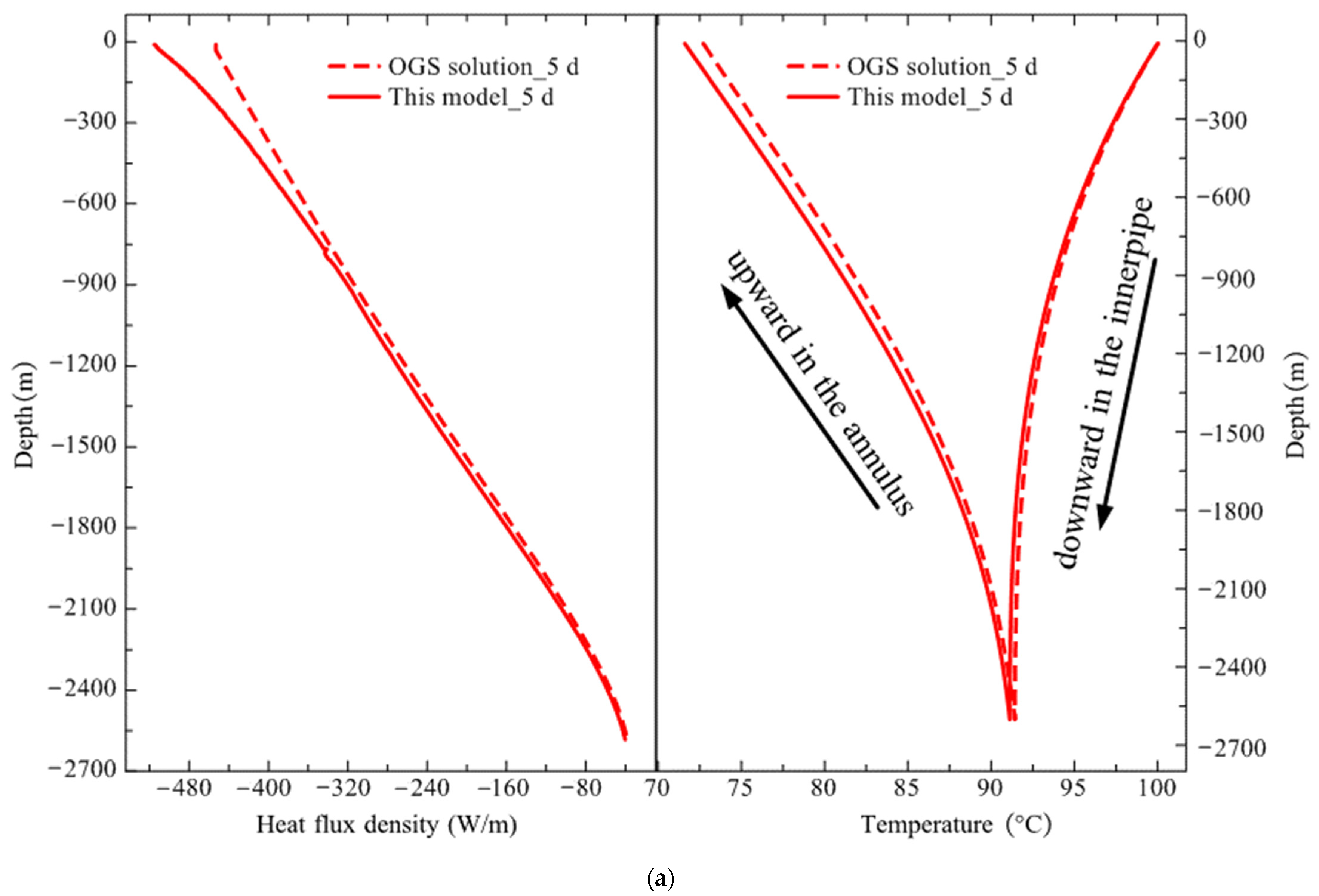
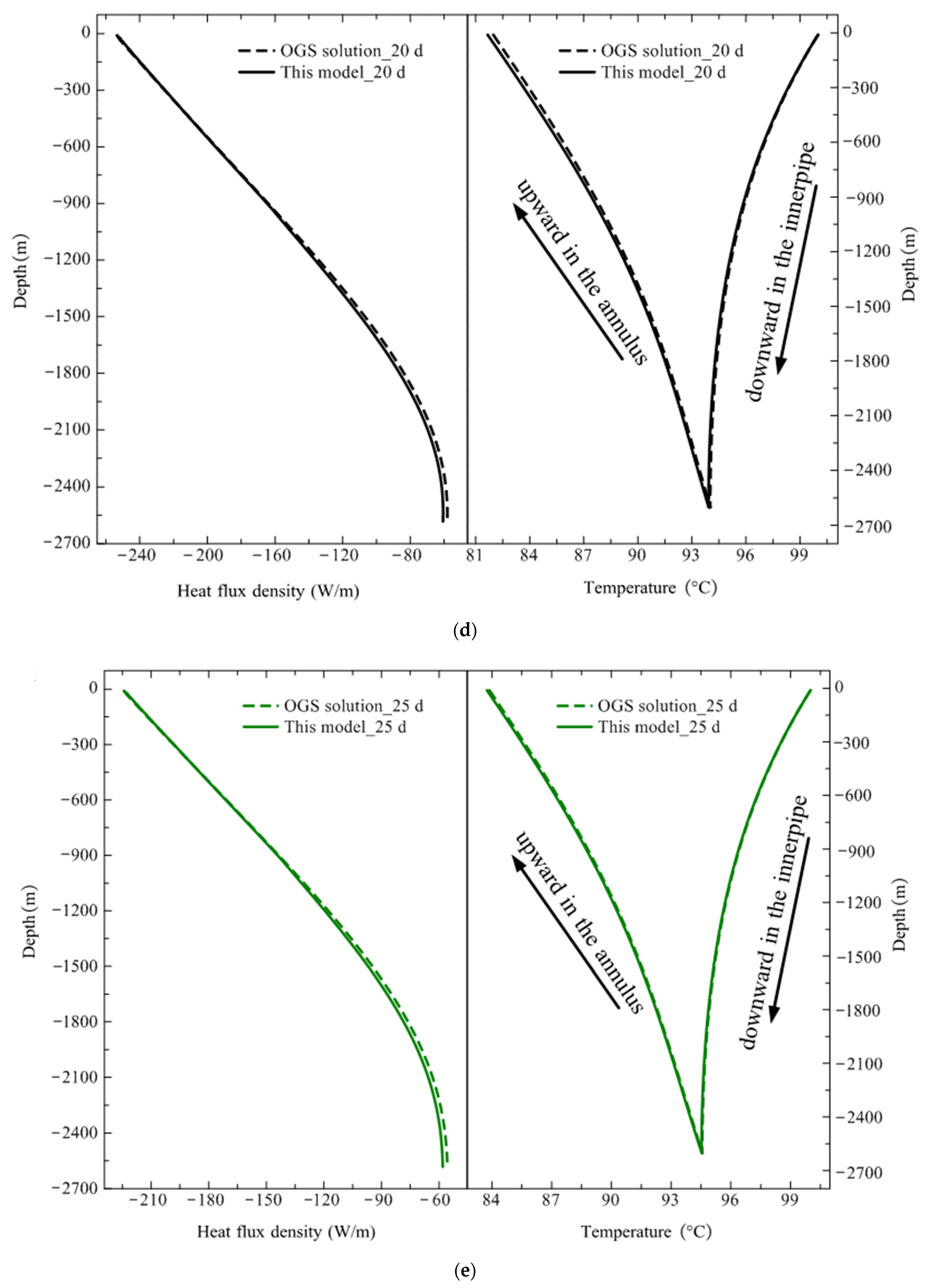
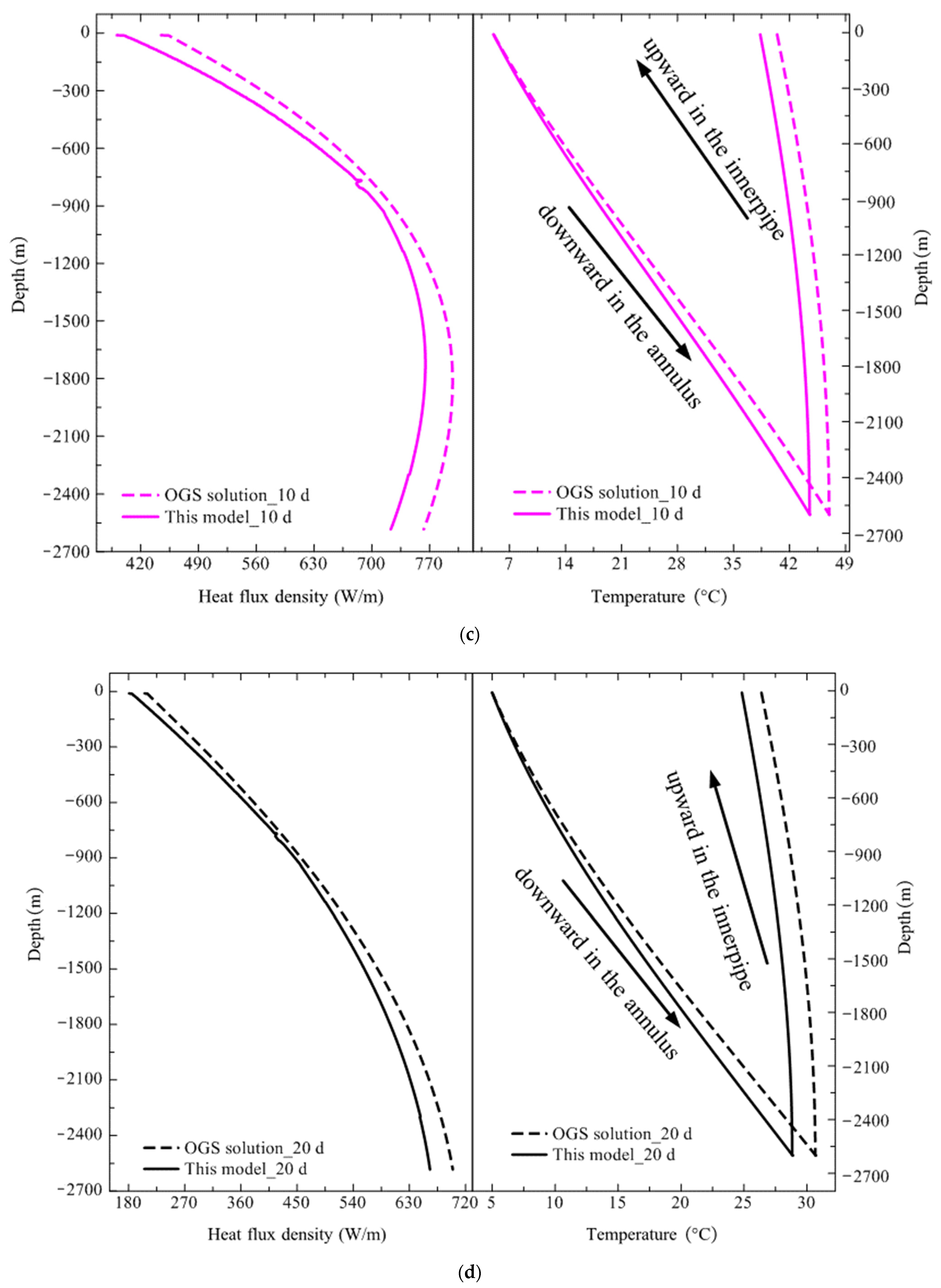
• Good accuracy: Through cross validation of the model in the typical high-temperature heat storage case, as well as the pilot demonstration project, large deviations are shown to mainly exist at the unsteady stage during the charging or discharging of DBHE, as shown in Table 3 and Table 10, while the simulation results are in excellent agreement with the OGS solution and field test data at the steady stage, according to Figure 8, Figure 9 and Figure 10. The prediction errors during both the charging and discharging phases are all around 5%, and they satisfy the accuracy requirement of engineering applications. Moreover, this model succeeded in depicting the dynamic evolution of extreme heat flux density and outlet water temperature in the pilot demonstration project, which was validated well against the OGS solution, as observed in Figure 11 and Figure 12. It could be seen that the large prediction error of the heat transfer model only existed in very short operation days during the initial unsteady stages of charging and discharging. Both relative errors under charging and discharging phases are within 5% during the steady state period. Hence, this model can simulate the challenging heat transfer problem with good accuracy.
• Easy implementation: No complex computations are involved in the overall simulation, as summarized in the flow chart of Figure 7. All the formulations are concise, without time-consuming iterations, which can be easily implemented by manual coding. In addition, this model could also be integrated into a HVAC system simulator such as TRNSYS or Energy-plus toolkits.
• High efficiency: Transient strong heat flux would appear during high-temperature charging and the subsequent discharging of DBHE. Extremely refined spatiotemporal resolution is required to capture the intense heat transfer, especially at the initial start-up. All the key physical laws of heat conduction in rock are formulated based on analytical solutions. Therefore, this model is featured with high computation efficiency in essence. Table 4 and Table 13 compare the simulation cost of both the charging and discharging phases of the deep BTES system, and demonstrate that our efficient heat transfer model achieves an acceleration ratio of 30 times, approximately relative to the fully numerical method.

4.2. Limitations of the Heat Transfer Model for Deep BTES

According to the mathematical formulations of rock temperature distribution within the thermal affecting radius and heat front propagation in Equations (5) and (6), it should be noted that this model is limited to the heat transfer modeling of a single DBHE. In view of the limited heat extraction potential, DBHE arrays would be necessary in practical applications where the heating demand of a building terminal is higher. In comparison with heat transfer of a single DBHE, thermal interference among DBHE arrays would arise as the heat fronts propagating from each DBHE interact with each other. Dynamic interaction during the propagation of more than one heat fronts proves to be quite complicated. It is impossible to be depicted analytically, but only simulated numerically. Additionally, this model is only intended for pure heat conduction in the rock without groundwater advection. However, active groundwater would flow around the DBHE in some scenarios where rock fractures are more developed. Under this condition, both heat conduction and heat convection should be properly considered in the mathematical modeling. This model is, thus, not applicable anymore. In the future, it is suggested to extend this heat transfer model to be capable of accounting for thermal interference among DBHE arrays and groundwater advection. The applicability of this model can be enhanced in more complicated engineering applications.

5. Conclusions

In this paper, we propose a generic and efficient heat transfer model for the transient heat transfer simulation of deep BTES during high-temperature charging and subsequent discharging phases. This model is an extension of our previous work on the heat transfer modeling of DBHE under single heat extraction condition. Firstly, we focused on the transient thermal analysis of DBHE under heat storage and heat extraction modes. It was discovered that the generic modeling of heat propagation outside the borehole in the rock zone could be achieved, since the heat conduction formulations prove to be universal. In addition, different operation modes of DBHE including charging and discharging could also be simulated by minorly altering the flow direction of circulating water inside the borehole. Secondly, the Hottel–Whillier steady-state model was applied to perform the heat transfer analysis within the solar collector during the charging phase. By coupling the solar collector with DBHE underground, overall transient heat transfer modeling on the integrated deep BTES system could be built. A typical high-temperature heat storage case from the literature and the pilot demonstration project in China were considered as benchmark test cases to validate the simulation accuracy and efficiency of this model. It was found that the large prediction error of the heat transfer model only existed in very short operation days during the initial unsteady stages of charging and discharging. By contrast, the prediction errors at the steady stage during charging and discharging are all around 5%, achieving a perfect agreement.

In comparison with single heat extraction by DBHE, high-temperature charging and discharging is typical of even a larger heat exchange temperature difference. Transient strong heat flux would appear around the borehole, which could be as high as 3000 W/m locally according to our simulation for the pilot demonstration deep BTES project during discharging. This is a rather challenging heat transfer problem to be simulated. It is not only computationally expensive, but also demanding in terms of robustness and stability for numerical methods. Despite the great challenge in the face of transient strong heat flux, this model was quite robust and succeeded in capturing the intense heat transfer during charging and discharging simulations. The dynamic evolution of both the heat flux density and outlet water temperature validated well against the OGS solution. Therefore, the credibility of this heat transfer model for the deep BTES system was fully demonstrated, which basically satisfied the accuracy requirement of engineering applications. The model accuracy for this case was summarized as following:

(1) During the charging phase, the prediction error for the average heat flux density was within 5% between the OGS solution and this model. The maximum error of heat flux density was 13.72% at the initial charging and 4.78% at the end. It could also be observed that the maximum error was located at the top section of the borehole during the initial charging from 5 to 15 days, and it moved toward the bottom from 20 to 30 days.

(2) During the discharging phase, the prediction error of the average heat flux density was also within 5%. Regarding the maximum prediction error in discharging, it was approximately 12% at the unsteady stage and 3.52% at the end. In addition, the maximum error was also located at the top section of the borehole within 5 days of the initial discharging. However, a larger prediction error occurred at both the top and bottom sections of the borehole during a transition period from 5 to 20 days of the discharging phase. Then, it gradually shifted to the bottom from 20 days to 120 days.

Moreover, the model is highly efficient compared to the traditional numerical method by OGS. A comparison of the simulation cost proved that this heat transfer model achieved an acceleration ratio of 30 times relative to the fully numerical method. In general, the heat transfer model proposed to perform the transient thermal analysis of the deep BTES system is accurate and efficient enough. It is promising for the design or optimization of a practical project.

The proposed method has four advantages: generic applicability, good accuracy, easy implementation, and high efficiency. However, this model is limited to the heat transfer of a single DBHE under pure heat conduction. It could not model thermal interference among DBHE arrays or the groundwater advection effect on heat transfer in the rock zone. Therefore, future research should focus on heat transfer characteristics under different layouts of DBHE arrays, as well as optimization on the heat storage efficiency through large scale DBHE arrays. In addition, more complicated heat transfer modeling coupled with groundwater flow in the porous media should also be studied, which could help to push this promising technology to real applications.

References

1. Rybach, L.; Hopkirk, R. Shallow and deep borehole heat exchangers-achievements and prospects. In Proceedings of the 1st World Geothermal Congress (WGC1995), Florence, Italy, 18–31 May 1995; pp. 2133–2139. [Google Scholar]
2. Sapinska, A.; Rosen, A.; Gonet, A.; Sliwa, T. Deep Borehole Heat Exchangers—A Conceptual and Comparative Review. Int. J. Air-Cond. Refrig. 2016, 24, 1630001. [Google Scholar] [CrossRef]
3. Kohl, T.; Brenni, R.; Eugster, W. System performance of a deep borehole heat exchanger. Geothermics 2002, 31, 687–708. [Google Scholar] [CrossRef]
4. Daniel, S. Simulation and Optimization of Medium Deep Borehole Thermal Energy Storage Systems. Ph.D. Thesis, Technische Universitat Darmstadt, Darmstadt, Germany, 2016. [Google Scholar]
5. Deng, J.W.; Wei, Q.P.; Liang, M.; He, S.; Zhang, H. Field test on energy performance of medium-depth geothermal heat pump systems (MD-GHPs). Energy Build. 2019, 184, 289–299. [Google Scholar] [CrossRef]
6. Bu, X.B.; Ran, Y.M.; Zhang, D.D. Experimental and simulation studies of geothermal single well for building heating. Renew. Energy 2019, 143, 1902–1909. [Google Scholar] [CrossRef]
7. Cai, W.L.; Wang, F.H.; Chen, S.; Shao, H.B. Analysis of heat extraction performance and long-term sustainability for multiple deep borehole heat exchanger array: A project-based study. Appl. Energy 2021, 289, 116590. [Google Scholar] [CrossRef]
8. Renaud, T.; Verdin, P.; Falcone, G. Numerical simulation of a deep borehole heat exchanger in the krafla geothermal system. Int. J. Heat Mass Transf. 2019, 143, 118496. [Google Scholar] [CrossRef]
9. Kristian, B.; Wolfram, R.; Bastian, W.; Daniel, S.; Sebastian, H.; Ingo, S. Seasonal high temperature heat storage with medium deep borehole heat exchangers. Energy Procedia 2015, 76, 351–360. [Google Scholar]
10. Bastian, W.; Wolfram, R.; Daniel, S. Characteristics of medium deep borehole thermal energy storage. Int. J. Energy Res. 2016, 40, 1855–1868. [Google Scholar]
11. Fang, L.; Diao, N.R.; Shao, Z.K.; Zhu, K.; Fang, Z.H. A computationally efficient numerical model for heat transfer simulation of deep borehole heat exchangers. Energy Build. 2018, 167, 79–88. [Google Scholar] [CrossRef]
12. Liu, J.; Wang, F.H.; Cai, W.L.; Wang, Z.H.; Wei, Q.P.; Deng, J.W. Numerical study on the effects of design parameters on the heat transfer performance of coaxial deep borehole heat exchanger. Int. J. Energy Res. 2019, 43, 6337–6352. [Google Scholar] [CrossRef]
13. Luo, Y.Q.; Guo, H.S.; Meggers, F.; Zhang, L. Deep coaxial borehole heat exchanger: Analytical modeling and thermal analysis. Energy 2019, 185, 1298–1313. [Google Scholar] [CrossRef]
14. Ma, L.; Zhao, Y.Z.; Yin, H.M.; Zhao, J.; Li, W.J.; Wang, H.Y. A coupled heat transfer model of medium-depth downhole coaxial heat exchanger based on the piecewise analytical solution. Energy Convers. Manag. 2019, 204, 112038. [Google Scholar] [CrossRef]
15. Zhao, Y.Z.; Pang, Z.H.; Huang, Y.H.; Ma, Z.B. An efficient hybrid model for thermal analysis of deep borehole heat exchangers. Geotherm. Energy 2020, 8, 18. [Google Scholar] [CrossRef]
16. Luo, Y.Q.; Yu, J.H.; Yan, T.; Zhang, L.; Liu, X. Improved analytical modeling and system performance evaluation of deep coaxial borehole heat exchanger with segmented finite cylinder source method. Energy Build. 2020, 212, 109829. [Google Scholar] [CrossRef]
17. Luo, Y.Q.; Cheng, N.; Xu, G.Z. Analytical modeling and thermal analysis of deep coaxial borehole heat exchanger with stratified-seepage-segmented finite line source method (S3-FLS). Energy Build. 2021, 257, 111795. [Google Scholar] [CrossRef]
18. Jordi, M. Large-Scale Underground Thermal Energy Storage Using Industrial Waste Heat to Supply District Heating. Bachelor’s Thesis, Universitat de Lleida, Lleida, Spain, 2014. [Google Scholar]
19. Wang, H.J.; Qi, C.Y.; Wang, E.Y.; Zhao, J. A case study of underground thermal storage in a solar-ground coupled heat pump system for residential buildings. Renew. Energy 2009, 34, 307–314. [Google Scholar] [CrossRef]
20. Diersch, H.; Bauer, D. Analysis, modeling and simulation of underground thermal energy storage (UTES) systems. In Woodhead Publishing Series in Energy, Advances in Thermal Energy Storage Systems; Woodhead Publishing: Sawston, UK, 2015; pp. 149–183. [Google Scholar]
21. Farzin, R.; Alan, F. Solar community heating and cooling system with borehole thermal energy storage-Review of systems. Renew. Sustain. Energy Rev. 2016, 60, 1550–1561. [Google Scholar]
22. Flynn, C.; Siren, K. Influence of location and design on the performance of a solar district heating system equipped with borehole seasonal storage. Renew. Energy 2015, 81, 377–388. [Google Scholar] [CrossRef]
23. Emil, N.; Patrik, R. Performance evaluation of an industrial borehole thermal energy storage (BTES) project-Experiences from the first seven years of operation. Renew. Energy 2019, 143, 1022–1034. [Google Scholar]
24. Xu, L.Y.; Torrens, I.; Guo, F.; Yang, X.D.; Hensen, J.L.M. Application of large underground seasonal thermal energy storage in district heating system: A model-based energy performance assessment of a pilot system in Chifeng, China. Appl. Therm. Eng. 2018, 137, 319–328. [Google Scholar] [CrossRef]
25. Gao, L.H.; Zhao, J.; An, Q.S.; Liu, X.; Du, Y. Thermal performance of medium-to-high temperature aquifer thermal energy storage systems. Appl. Therm. Eng. 2019, 146, 898–909. [Google Scholar] [CrossRef]
26. Gao, L.H.; Zhao, J.; An, Q.S.; Liu, X. A review on system performance studies of aquifer thermal energy storage. Energy Procedia 2017, 142, 3537–3545. [Google Scholar] [CrossRef]
27. Hellstrom, G. Ground Heat Storage Thermal Analysis of Duct Storage Systems. Ph.D. Thesis, University of Lund, Lund, Sweden, 1991. [Google Scholar]
28. Yang, H.; Cui, P.; Fang, Z.H. Vertical-borehole ground-coupled heat pumps: A review of models and systems. Appl. Energy 2010, 87, 16–27. [Google Scholar] [CrossRef]
29. Zhang, F.F.; Fang, L.; Jia, L.R.; Man, Y.; Cui, P.; Zhang, W.K.; Fang, Z.H. A dimension reduction algorithm for numerical simulation of multi-borehole heat exchangers. Renew. Energy 2021, 179, 2235–2245. [Google Scholar] [CrossRef]
30. Huang, Y.; Zhang, Y.; Xie, Y.; Zhang, Y.; Ma, J. Field test and numerical investigation on deep coaxial borehole heat exchanger based on distributed optical fiber temperature sensor. Energy 2020, 210, 118643. [Google Scholar] [CrossRef]
31. Hu, X.C.; Banks, J.; Wu, L.P.; Liu, W.V. Numerical modeling of a coaxial borehole heat exchanger to exploit geothermal energy from abandoned petroleum wells in Hinton, Alberta. Renew. Energy 2020, 148, 1110–1123. [Google Scholar] [CrossRef]
32. Wang, Z.H.; Wang, F.H.; Liu, J.; Ma, Z.J.; Han, E.S.; Song, M.J. Field test and numerical investigation on the heat transfer characteristics and optimal design of the heat exchangers of a deep borehole ground source heat pump system. Energy Convers. Manag. 2017, 153, 603–615. [Google Scholar] [CrossRef]
33. Zhao, Y.Z.; Ma, Z.B.; Pang, Z.H. A fast simulation approach to the thermal recovery characteristics of deep borehole heat exchanger after heat extraction. Sustainability 2020, 12, 2021. [Google Scholar] [CrossRef] [Green Version]
34. Duffie, J.A.; Deckman, W.A. Solar Engineering of Thermal Process; John Wiley and Sons: New York, NY, USA, 1980. [Google Scholar]
Figure 1. Schematic of model development in this study.
Sustainability 14 09702 g001
Figure 2. Heat flux evolution during high-temperature charging and discharging of DBHE.
Sustainability 14 09702 g002
Figure 3. Heat storage for charging and heat extraction for discharging of DBHE.
Sustainability 14 09702 g003
Figure 4. Quasi-steady state heat transfer analysis inside the borehole for charging of DBHE.
Sustainability 14 09702 g004
Figure 5. Quasi-steady state heat transfer analysis inside the borehole for discharging of DBHE.
Sustainability 14 09702 g005
Figure 6. High-temperature heat storage for DBHE supplied by solar collector.
Sustainability 14 09702 g006
Figure 7. Flow chart for heat transfer simulation of deep BTES under charging or discharging phase.
Sustainability 14 09702 g007
Figure 8. Comparison of high-temperature heat storage performance of DBHE based on the proposed model, OGS simulation results and literature data: (a) evolution of outlet temperature; (b) evolution of heat exchange output.
Sustainability 14 09702 g008aSustainability 14 09702 g008b
Figure 9. Evolution of inlet and outlet temperature for the deep BTES system during charging phase from in situ field test and simulation results of the model.
Sustainability 14 09702 g009
Figure 10. Evolution of inlet and outlet temperature for the deep BTES system during discharging phase from in situ field test and simulation results of the model.
Sustainability 14 09702 g010
Figure 11. Comparison of simulation results of heat flux density and circulating water temperature distribution along borehole depth during the charging period: (a) 5 days; (b) 10 days; (c) 15 days; (d) 20 days; (e) 25 days; (f) 30 days.
Sustainability 14 09702 g011aSustainability 14 09702 g011bSustainability 14 09702 g011cSustainability 14 09702 g011d
Figure 12. Comparison of simulation results of heat flux density and circulating water temperature distribution along borehole depth during the discharging period: (a) 1 days; (b) 5 days; (c) 10 days; (d) 20 days; (e) 30 days; (f) 40 days; (g) 50 days; (h) 120 days.
Sustainability 14 09702 g012aSustainability 14 09702 g012bSustainability 14 09702 g012cSustainability 14 09702 g012d