Using ABM to Study the Potential of Land Use Change for Mitigation of Food Deserts

Abstract

Land-use transition is one of the most profound human-induced alterations of the Earth’s system. It can support better land management and decision-making for increasing the yield of food production to fulfill the food needs in a specific area. However, modeling land-use change involves the complexity of human drivers and natural or environmental constraints. This study develops an agent-based model (ABM) for land use transitions using critical indicators that contribute to food deserts. The model’s performance was evaluated using Guilford County, North Carolina, as a case study. The modeling inputs include land covers, climate variability (rainfall and temperature), soil quality, land-use-related policies, and population growth. Studying the interrelationships between these factors can improve the development of effective land-use policies and help responsible agencies and policymakers plan accordingly to improve food security. The agent-based model illustrates how and when individuals or communities could make specific land-cover transitions to fulfill the community’s food needs. The results indicate that the agent-based model could effectively monitor land use and environmental changes to visualize potential risks over time and help the affected communities plan accordingly.

1. Introduction

Research in regional and local food systems has gained significant attention. Multiple studies have investigated individuals and entities involved in food systems regarding decision-making behavior, strategies, interactions, and the impacts of the interlinkages between the components of the systems [1,2,3]. From the modeling perspective, local and regional food systems often refer to the shorter supply chain with a specific focus on the geographic proximity of producers, consumers, and the affected communities [4,5].

A food system represents a complex web of decisions, actions, and consequences involving a collaborative process from production to supply chain and consumption. The literature points to the many issues and challenges within such an intertwined system and specifically notes the common lack of effective governance, distribution, communication, and resource allocation in inefficient food systems [6,7]. The studies related to food deserts are good examples, often demonstrating the combinations of the challenges regarding food availability, access, utilization, and accountability [8,9,10].

Accessibility to healthy, affordable, high-quality food has long been a challenge in low-income, urban, and rural areas across the US and globally [11,12]. In addition, many people continue to struggle with food price inflation, and supply issues recently brought on by the COVID-19 pandemic. Everything from demand for healthy foods to export and import challenges has hit many communities. As a result, low-income households, the elderly, and children are more vulnerable to an increasingly pervasive state of food insecurity.

In most general terms, food deserts are defined as geographic areas characterized by both low income and low access to nutritious food [13]. A recent study showed that about 795 million people in the world have limited access to healthy food, and most of these live in developing regions of the world [14]. This is also a severe issue in developed countries. For example, nearly 39.5 million people (12%) of the U.S. population were living in low-income and low-access areas, according to the USDA’s most recent data [15]. Similarly, in the U.K., 10% of the population were living in food insecurity in 2016, whereas about 13% of Canadians were food insecure in 2018. These levels of limited access to healthy foods are also common in other affluent countries.

Multiple studies have related low consumption of fresh fruits and vegetables to elevated risks of various chronic diseases, including heart disease, stroke, and diabetes [16]. Moreover, since limited access to supermarkets, supercenters, grocery stores, or other sources of healthy and affordable food is posited to be one of the critical barriers for households to eat a healthy meal, research documenting the link between populations living in food deserts having higher risks of battling chronic health issues has been growing [17,18].

Various factors contribute to food deserts, including income [19], political instability [20], access to transportation and supermarkets, and shortage of agricultural production due to climate variability, soil quality, and population growth [21]. Climate variability and soil quality significantly affect the quality and quantity of the agricultural output via routes such as drowned crops and lower yields [22,23]. Moreover, the rapid global human population growth can also impact the food supply and access in the future. Therefore, increasing the agricultural output is essential to meet the needs across the globe, especially in developing countries.

However, local farmer’s markets can serve as community-level interventions, bringing healthy and affordable food options to the food deserts community [24]. They are one promising way to address the nation’s chronic health problems associated with less fruit and vegetable consumption. Moreover, they can connect the rural to the urban, farmer to consumer, and fresh ingredients to our diets and become economic and community centerpieces in cities and towns across the U.S. These markets can be developed in communities with low-income, minority communities, and communities with limited access to healthy and affordable foods.

Understanding how the interactions between households and the food environment lead to sufficient fresh fruits and vegetable consumption is critical to overcoming healthy food insecurity. Understanding how land-use transitions interrelate with households’ decisions and the environmental conditions is vital to predicting the impacts of potential economic scenarios and land-use planning and policy [25,26]. Intentional land-use transition can support better land management and decision-making for increasing the yield of food production to fulfill the food needs in a specific area. To inform the policymaking, modeling land-use changes needs to reflect the complexity of both its human drivers and natural or environmental constraints [27]. In addition, changes on the macro level, such as global policies and population growth, can affect individuals’ behavior, creating changes at the micro-level [28].

Monitoring vegetation/crop conditions and land-use transition maps can be created using remote sensing-based indexes [29,30] and model-based approaches [31,32,33,34]. The remote sensing indexes approach has been widely used to monitor the vegetation/crop conditions at regional and global scales at various spatial and temporal resolutions. One commonly used remote-sensing index for measuring vegetation conditions is the vegetation condition index (VCI) [29]. The vegetation conditions can be attributed to the disaster’s impact on vegetation/crops. The Disaster Vegetation Damage Index (DVDI) is another index-based approach used effectively to measure a disaster’s effects on vegetation/crops [30].

Several main methods have been proposed for modeling land use and land cover changes, such as Markov chain models [31], system dynamics [32], microsimulation models [33], and agent-based models (ABM) [34]. The Markov chain model is an essential projection model that has been used to model land-use changes at large spatial scales [35]. This approach can study different states’ initial occupation and transition probabilities to determine the development trend and predict the future state, especially when the changes and processes in the land are difficult to describe. However, it is limited for predicting spatial patterns because the approach utilizes only limited spatial knowledge. Additionally, Markov chain models often assume that dynamic processes evolve following the same (stationary) probabilities as observed in the recent past [36,37].

The system dynamic method uses feedback loops, accumulations, time delays, flows, and stocks to understand the complex system’s nonlinear behavior over time. This approach is based on the idea that all of the dynamics occur as a result of the accumulation of flows in stocks. System dynamic has a top-down simulating structure that can avoid one-sided thinking limitations and enable understanding of the whole structure behind a complex phenomenon. However, it cannot effectively examine the driving forces of land-use changes and the impact of human system behavior on the environment due to its structure, which does not account for micro-level dynamics [32]. In contrast with the system dynamics approach, microsimulation models analyze the land and the population dynamics at a micro-level based on individuals (or agents) [33,38]. This approach is based on individual-level or microdata relating to the characteristics and behaviors of individuals. Such models have a bottom-up structure that describes agents with individual data (e.g., population census data) and simulates their behaviors with transition probabilities produced from the data. However, the interaction between individuals is ignored in this approach.

The fourth main approach, the ABM, has emerged as a potent tool to model various dynamic processes, including food security [39,40], agricultural policy evaluation [41], and urban planning [42]. For example, Natalini et al. [39] developed the ABM that simulates the global food market and the political fragility of countries. The model effectively simulates the effects of food insecurity on international food prices and how these increase food riots in countries. The model can also be used to simulate the consequences of food riots. Similarly, Namany et al. [40] used the ABM to simulate the perishable food market strategies under different circumstances for a Qatar-based case study. The ABM developed effectively simulates the performance of the tomato market in the state of Qatar under different economic and environmental scenarios. Wossen et al. [41], on the other hand, used the ABM to analyze how adaptation affects the distribution of household food security and poverty under the current climate and price variability. They also examined the effectiveness of policy interventions for promoting agricultural credit and off-farm employment opportunities. Their experiments suggest that the ABM is an effective tool for the analyzes of climate and price variability’s effect on household welfare.

The ABM has also become an essential tool for exploring potential land system developments, especially when hypothetical scenarios have not yet been observed in the real world [34,43,44]. ABM assumes a collection of autonomous decision-making entities called agents. The agents in the ABM are independent, autonomous units with properties and actions that attempt to fulfill a set of goals. The agents do not have to represent humans. Instead, they can be land, farmers, or households in the land-use transition context. Each agent individually assesses their situation and makes decisions based on a set of rules. Furthermore, the agents can interact with each other and their environment, resulting in emergent outcomes at the macroscale level [45]. These interactions can be direct (e.g., communication and physical interaction) or indirect (e.g., via multiple-pathway feedback and aggregate results).

Compared to conventional modeling approaches, ABMs are often more complex and difficult to generalize beyond a specific context because they depend on local knowledge and data [46]. However, due to the ABM bottom-up model structure, they have a vital role in examining the driving forces of land-use changes and the impact of human system behavior on the environment [47]. In addition, the ABM allows high heterogeneity in agent characteristics and interactions between agents and environments and features like dynamics, feedback, and adaptation, which are impossible to represent in conventional models. For land-use application, the ABM offers a way of incorporating the influence of human decision-making on land use in a formal and spatially explicit way and modeling individual decision-making entities and their interactions since they are based on individual agents [48,49,50]. However, to our knowledge, the ABM has not been applied to specifically study land-use transitions as influenced by and influencing food deserts.

To fill the gap in the understanding of how the ABM approach could be used to study land-use transitions in the context of food deserts, this study (1) outlines the major steps for the development of an ABM that accounts for the interrelationships between relevant human and natural systems, (2) identifies the crucial information needed to make the ABM operational, and (3) demonstrates the feasibility of such modeling for a chosen county in the state of North Carolina, U.S., based on publicly available data and estimated functional relationships published to date. The study is motivated by the following questions: how can the interaction between households and the food environment lead to adequate fresh fruits and vegetables? How do climate variability, soil quality, population growth, and policies lead to crop insecurity over time? How does land use transition lead to adequate healthy and affordable food access for the local community? How would maximizing crop production within or around the food desert communities in the study area improve households’ food access? The study itself is not about the ABM. Instead, it applied the ABM to show the relation between food needs and production and the potential of land use transition to meet the food needs to overcome food desert.

Our methodology adopts a multi-disciplinary approach looking at several food desert indicators to achieve sustainable crop provision and meet the food needs. The main agents that contribute to crop yield reduction and food desert factors such as climate variability, soil quality, and population growth impacts are incorporated in the model. The framework uses monthly data as an input to simulate the component behaviors and create sustainable strategies aimed at satisfying the local food needs. The study hypothesis is that the interaction between households and the food environment and land use transition lead to adequate fresh fruits and vegetables. Moreover, significant climate variation and population growth rate affect the crop production output and food demand each season. We assumed the households would not change their purchasing pattern and consumption preferences dramatically in any given time period, which means the fruit and vegetable consumption mentioned in our study would remain constant throughout the county. The study approach can guide stakeholders, policymakers, and other responsible agencies to sustain or improve communities’ livelihoods and food security. Furthermore, the system approach proposed to develop the framework can be adopted and used for future research to test the effectiveness of land-use and land-cover changes to meet the food needs globally.

The paper is organized as follows: Section 2 introduces the methods used. Section 3 presents the study area and research data along with data processing. Section 4 presents the results and discussions. Finally, Section 5 presents the conclusion of the study.

2. Methods: Model Development

This section describes the ABM development to simulate the behavior of human and natural systems in land use transition to improve healthy food security. The study approach required an iterative development process with several phases and data preparation incorporated into each.

Agent-based modeling is a bottom-up computer simulation technique used to analyze a system by its individual agents that interact with each other, for example, the interactions between people, things, places, and time. The agents are programmed to behave and interact with other agents and the environment in certain ways. These interactions produce emergent effects that may differ from the effects of individual agents. Agents are a representation and a simplification of complex behavior, such as human behavior. This representation is established by defining rules, which the agent uses to achieve specific goals. The rules together represent the ‘rational’ behavior of the agent. To simulate an agent model, we let the agents communicate with each other and other agents. Communication in agent simulation is how an agent modeler intuitively sees the interactions between real-life (e.g., other agents, but also the environment) entities. Agents must be able to communicate with each other, dependent on the behavior-rules one applies in the model; also, agents communicate with the simulated environment. They can be represented with rules that allow them to learn and copy their neighbors and have a decisional structure obtained from “frames of reference”.

ABMs can offer a way of incorporating the influence of human decision-making on land use in a mechanical, formal, and spatially explicit way, considering social interaction, adaptation, and decision-making at different levels. In this research, the systems that affect a community’s food security are categorized into two major groups: (I) human systems such as households, and (II) natural systems such as land agents, which produce ecosystem services affecting or fulfilling the human agents’ needs. The ABM is applied to analyze the influence of the behavior of individual human system agents (farmers, households, consumers) on the emergent properties of the natural system agent, such as landscape. This model can be used to create realistic representations of food desert indicators, such as climate variability, soil quality, population growth, and policies. Figure 1 shows the conceptual model of farmland use change and interaction between household agents and natural systems.

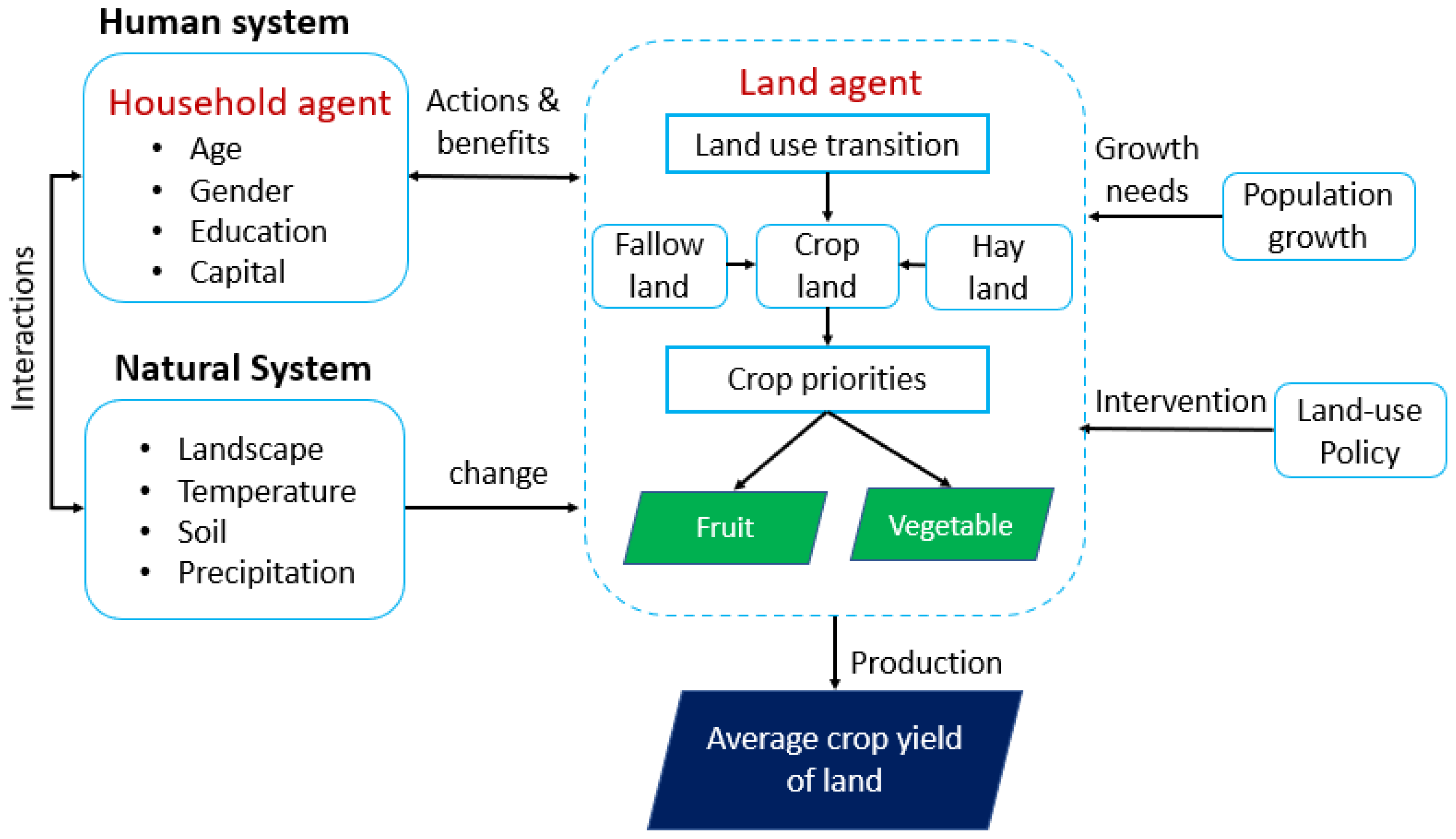
• Human System. The human system comprises individuals and households and their decision-making and actions upon farmland use. The study used age and gender to estimate the food needs of the population in the county. These allowed us to estimate households’ fruit and vegetable needs based on the Centers for Disease Control and Prevention (CDC) daily recommendations. In this study, household agents define the human system. Therefore, household agents are minimal units for measuring human variables and include household information and land perceived by the agents, which are either farming or consumer households. A farming household is a household that decides how to use its farmlands and allocate resources at the beginning of the farming season. In contrast, a consumer household is a household with its own behavior and decision-making characteristics when it comes to consuming food items such as fresh fruits and vegetables. The food choice of each consumer household is influenced by the type of crops that the farming household grows. The main attributes of households include human, physical, and natural-related factors. Each individual who belongs to the household is defined by their age, gender, income, and educational status. The household’s agent structure is described as:

  $$Household agent \left(H\right)=\left\{H_{backgroud}, Lan{d}_{information},H_{behavior},Rules, Decision \right\}$$

  (1)

  where, $H_{backgroud }$ is a set of household information including individual variables; $Lan{d}_{information}$ is the spatial information obtained from lands, such as plot land size; $H_{behavior}$ is behavioral parameters that the households or individuals use to make decisions; Rules are a set of conditions that define a logical procedure driven to decide how households use their land parcels. It represents the Decision-making mechanism that takes inputs from the household’s background and land parcels, assuming that household agents behave reactively according to the rules. A procedure of decision-making is universal for all household agents concerning its logical sequence. However, decision outcomes are diverse since the agent’s state, parameters, and structure of utility functions are individual-specific. The household background included the following attributes as mentioned before:

  $$H_{backgroud}=\left\{H_{human, } H_{parcel lands, } H_{policy, }, H_{capital, } H_{size, }{H}_{education status }\right\}$$

  (2)

  where, $H_{human }$ represents the human resources based on their age and gender, $H_{parcel land }$ is the available land, $H_{capital }$ represents farm landowners’ capital, $H_{policy}$ is policy related to households and their land uses, $H_{size }$ represents households size, and $H_{education status }$ is the educational status of landowners or households.
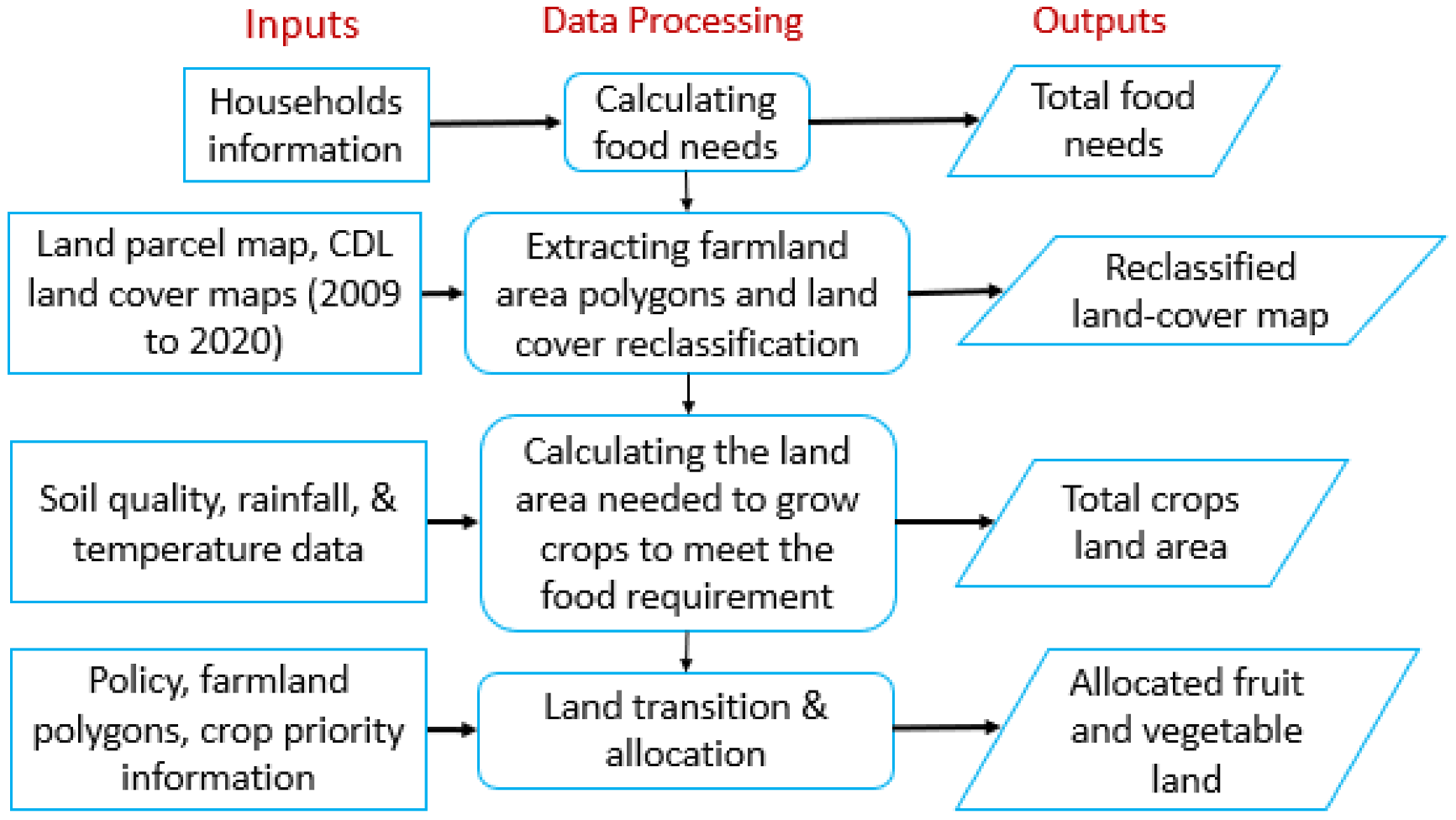
• Natural System. The natural system is the landscape with its attributes and ecological response mechanisms to environmental changes and human interventions (Figure 1). The study selected the main natural system-related factors contributing to a food desert based on literature and data availability. These include landscape, temperature, soil quality, and precipitation. For example, temperature and precipitation variability adversely affect the quality and quantities of crop production. In addition, soil quality also has a significant impact on crop production. In this study, land agents define the natural system. A land agent is a spatial unit for measuring spatial variables of a landscape corresponding to a parcel map, such as land cover and property boundaries.

  $$Land aget \left(L\right)=\left\{ Land size, Climate varablity, Soil quality\right\}$$

  (3)

  Land size is the total available farmland used by farmers to produce fruits and vegetables needed to meet the food requirements. Since the unavailability of enough land for crop production causes a shortage of healthy foods, the model makes a land-use transition to minimize the issue. In this case, the land-use change is made by considering regional and federal land use policies, Climate variability, and Soil quality. For example, since temperature and precipitation affect the crops’ planting, growing, and harvesting processes, the model considers these factors to estimate the size of croplands needed to meet the food requirements and the amount of crop yields obtained from the farmlands. Soil is another essential element of thriving agriculture and is the primary source of nutrients used to grow crops [51]. Soil quality affects the quality and quantity of crop production. Farmlands with relatively healthy soils produce healthy and high amounts of fruits and vegetables. Based on that context, the fruit and vegetable yields obtained per acre of land can be estimated by considering the land’s soil quality. The decision is based on the agents’ expected yields, land availability, and the fruit and vegetable needs of the community. Therefore, food needs are considered by simultaneously optimizing the production and consumption decisions. Note that landscape, temperature, soil, and precipitation are selected for the natural system based on literature and availability of data.
• The interaction of human and natural systems. The human and natural systems’ interactions drive land-use changes critical for global processes such as climate change and food shortage. The human system impacts natural systems, whereas natural systems present food production conditions to the human system. The human system affects the natural environment in many ways, including pollution and deforestation. These changes have resulted in climate change and a shortage of rainfall that have led to food insecurity [52]. In this research, through our ABM model, we study the interaction between these two systems and farmland-use transition in response to human decisions and natural constraints to improve food deserts. This interaction can be between human agents or human–natural agents. For example, the interaction between human and natural agents can affect the quality and quantity of farmland’s crop yields. Natural agent attributes such as temperature, rainfall availability, and soil quality affect the farm’s crop productivity. The ABM model can simulate this interaction and show possible solutions to increase crop production by implementing land-use changes. The land-use changes can allow the use of more farmlands to increase crop yields when there is not enough rainfall, temperature, and the soil quality of the farmland is not good.

Each individual’s daily vegetable and fruit needs can be calculated based on health officials or other responsible agencies’ recommendations. This research used the CDC daily health food intake recommendation and calculated the amount of healthy food intake by considering an individual’s gender, age, and health status. Then, the size of the farmland area to grow the food requirements are calculated under different conditions, such as considering crop type or the suitable season to grow that crop. The calculations also consider the condition of rainfall, temperature, and soil quality. The detailed procedure of the ABM development is presented in the next section.

3. Data Processing

The ABM was implemented on NetLogo, a multi-agent programming modeling environment [53]. In addition, ArcGIS was used for preprocessing the input data.

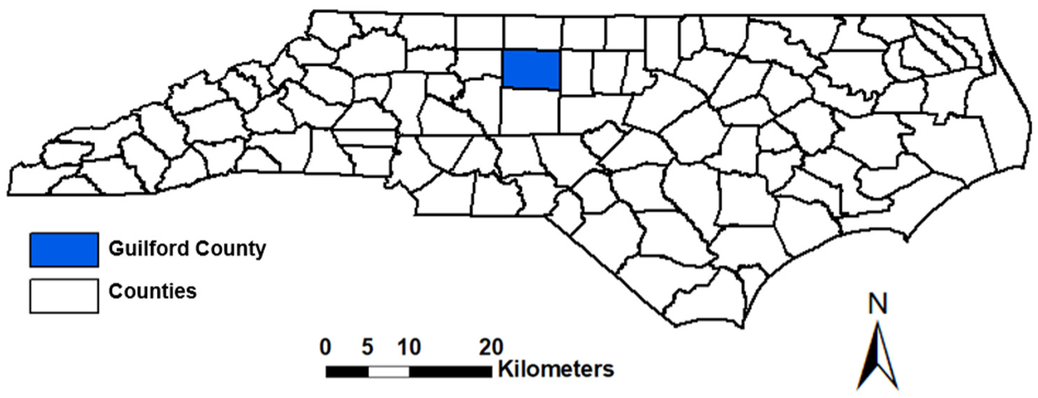
3.1. Study Area

Guilford County, North Carolina, U.S., is selected as a study area for the research because most of its population is in food deserts. The study area is shown in Figure 2. Guilford County is the third-most populated county in the state of North Carolina. It is a part of the Piedmont Triad and is located in the north-central area of the State. This county has historically served as one of Southeast’s significant manufacturing and transportation hubs. According to U.S. Census Bureau, Guilford County’s 2017 estimated population was 526,953 compared to 488,406 in 2010. According to 2017 estimates, there were an estimated 203,199 total households in Guilford County. This county has the same average household size of 2.5 persons as North Carolina as a whole. According to County Health Databook, North Carolina State Center for Health Statistics, life expectancy at birth in Guilford County is 78.4 years, higher than in the state as a whole; however, life expectancy has declined in Guilford County over the last several years.

The USDA Food Access Research Atlas maps census tracts that have both low income and low access information, as measured by the different distance demarcations [54]. For the purposes of this tool, the definition of low access to food is interpreted as being in a low-income census tract, and census tracts are regarded to have low access if a large share of people in the tract are “far from a supermarket, supercenter, or large grocery store”. The Atlas allows for multiple ways to depict the characteristics that can contribute to food deserts, including income level, distance to supermarkets, and vehicle access. Figure 3 shows the 2019 food desert tracts of Guilford County created using the USDA “1and10” food desert mapping definition in this study. According to the “1and10” USDA definition, a census tract is designed as a food desert when it fulfills the following requirements: (1) if the poverty rate becomes 20% or greater, or a median family income is at or below 80% of the statewide or metropolitan area median family income, and (2) if at least 500 persons and at least 33% of the population live more than 1 mile to the nearest supermarket or grocery store in the urban areas and more than 10 miles in the rural areas. Based on that definition, 263,826 (54%) people out of the total population of 488,406 are in the food desert, i.e., most people in the county have limited access to healthy and affordable foods.

According to USDA’s 2017 report, this county included 900 farmlands with an average size of 89 acres. The total number of agricultural producers is 1374, including 887 males and 487 females. Out of all producers, some 114 are aged less than 35, 762 aged 35–64, and 498 aged 65 and older. Recent data shows that land on farms declined significantly in this county from 1987 to 2017 (Figure 4), leading to a reduced agricultural production.

As shown in Figure 4, in 1987, there were 126,369 acres of farmland, yet the farmland decreased to 76,352 acres (by 40%) in 2017. Several factors caused this farmland loss in the county, including soil degradation, climate change, and the expansion of urbanization. For example, soil degradation can cause vegetation cover removal from soils and loss of land minerals [55]. In addition, urbanization has led to the continuous expansion of built-up areas and urban population growth, leading to farmland reduction [56].

3.2. Research Data

The following datasets were used for developing the land-use transition model in this study:

• Annual rainfall and temperature data. Annual precipitations and temperature data for the study area were downloaded from the U.S. Geological Survey (USGS) website (https://waterdata.usgs.gov/nc/nwis/annual/?referred_module=sw (accessed on 8 June 2021)) and National Oceanic and Atmospheric Administration (NOAA) website (https://www.ncdc.noaa.gov/cdo-web/ (accessed on 2 June 2021)). The precipitation record comes from human-facilitated and automated observation stations in the Global Historical Climatology Network-Daily database. The study used the annual rainfall and temperature data from the year 2011 to 2020 for model development purposes.
• Cropland Data Layer (CDL) data. The CDL land cover raster was downloaded from the USDA website (https://nassgeodata.gmu.edu/CropScape/ (accessed on 26 June 2021)). CDL is a publicly available land cover classification map covering 48 states in the U.S. at 30 m resolution. The study used the CDL raster from 2011 to 2020 for land cover analysis purposes.
• Parcel data. The parcel data has information about Guildford County property ownership. The data was downloaded from the NC OneMap website (https://www.nconemap.gov/ (accessed on 15 July 2021)).
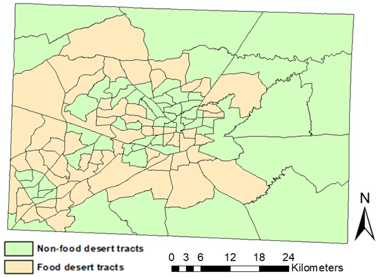
• Household data. The household data for Guilford County was downloaded from the USDA Economic Research Service website (https://www.ers.usda.gov/data-products/food-access-research-atlas/ (accessed on 12 June 2021)). The Food Access Research Atlas has an overview of food access factors for low-income and other census tracts using various measures of supermarket accessibility. It also provides food access data for populations within census tracts. The study used this data to create a food desert map of Guilford County. This study also used household information such as an individual’s gender and age to estimate the total food requirement of a specific area since individual daily fruit and vegetable needs depend on them. In addition, since we use an ABM, a bottom-up strategy, data containing the spatial distribution of households and their characteristics in our study area are used for model development.
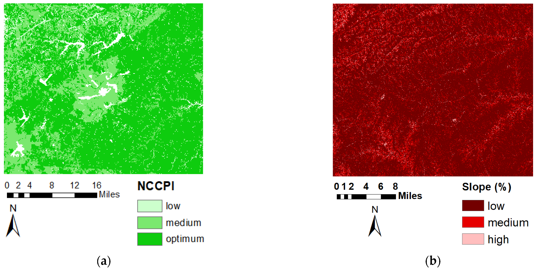
• Soil data layer. This layer displays the National Commodity Crop Productivity Index (NCCPI) derived from the Soil Survey Geographic Database (SSURGO). SSURGO is generally the detailed level of soil geographic data prepared by the National Cooperative Soil Survey (NCSS) in accordance with the NCSS mapping standards. The soil quality data ranks the inherent capability of soils for crop production and other applications. This data was downloaded for our study area from the NCCPI in ArcGIS online (https://landscape11.arcgis.com/arcgis/ (accessed on 15 July 2021)). This map has 30 m pixel size and, combining this layer with other information, is used to measure soil suitability for crop production in this study.
• Population growth rate data. The population growth data was collected for Guilford County, North Carolina, from 2011 to 2020 as input for the ABM development. This data was used to estimate the seasonal fruit and vegetable needs of Guilford County. The data was downloaded from the United States Census Bureau website (https://www.census.gov/data.html (accessed on 15 June 2021)).

3.3. Data Processing

In this stage, data preprocessing such as mapping, georeferencing, resampling, and reclassification is done for the model development purposes. Each data preparation and processing task is presented below:

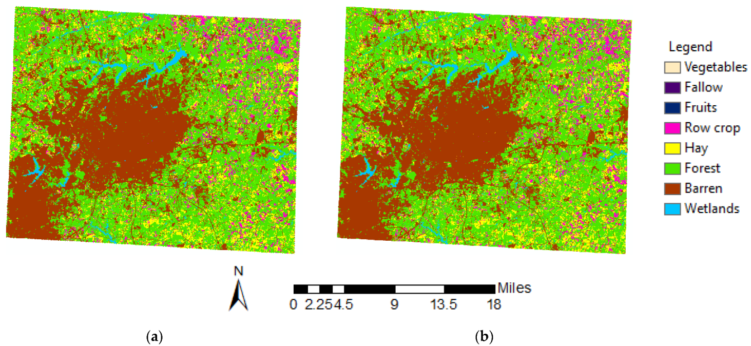
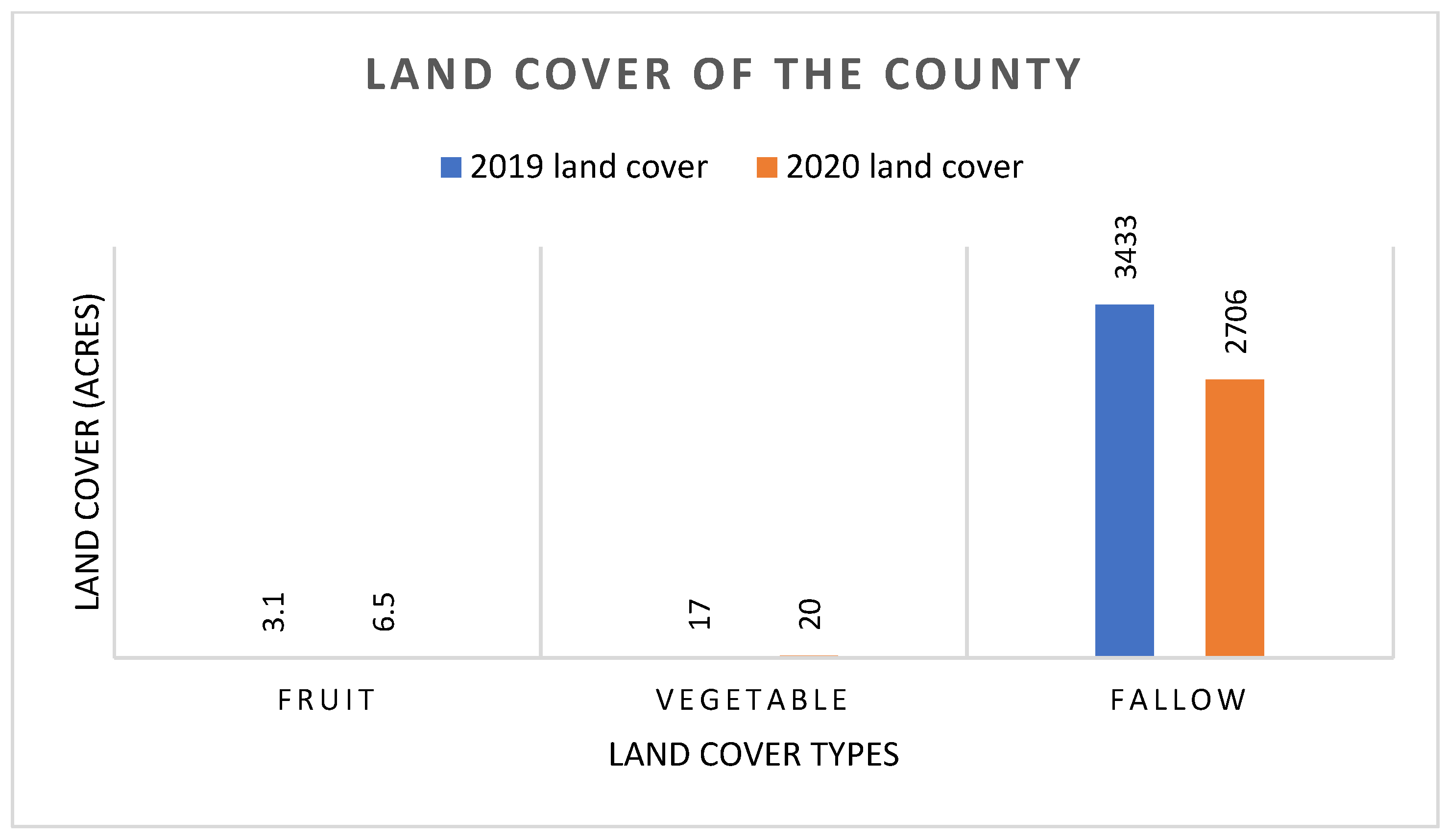
• CDL Data Reclassification. The study reclassified the CDL maps of Guilford County downloaded from the USDA website from 2019 to 2020 to use them as input for the ABM development. The CDL map layers have more than 120 individual classes, including apple, carrot, orange, cabbage, etc. The reclassification is done to group all types of fruit together as one class, “fruit”. The same regrouping process is done to combine all vegetables as one “vegetable” class [57]. Based on that context, each season, CDL’s farmlands (from 2011 to 2020) were regrouped into eight categories: (1) vegetable, (2) fallow, (3) fruit, (4) row crop, (5) hay, (6) forest, (7) barren, and (8) wetlands.
• Georeferencing and Resampling the Data. In this study, we clipped the Guilford County CDL raster layer from the North Carolina CDL map for further analysis. In addition, the raster data used in the study were georeferenced for geospatial data integration and visualization purposes.
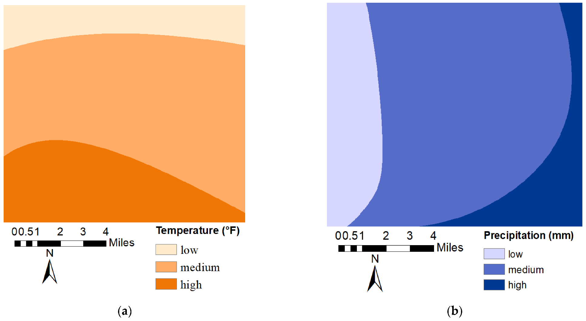
• Precipitation, temperature, and slope maps preparation. Temperature and rainfall raster maps were generated to understand their effects in Guilford County. We used point temperature and rainfall data to create these spatially distributed heat maps using the Kriging interpolation method with a 30 m pixel resolution. Kriging is a geostatistical procedure that creates an estimated surface from a scattered set of points with values. The slope map for the study area was also created using the interpolation method to understand the nature of the study area’s land for farming.
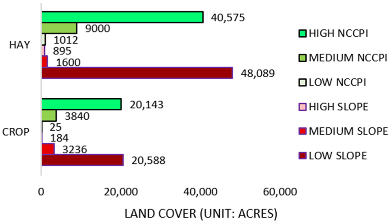
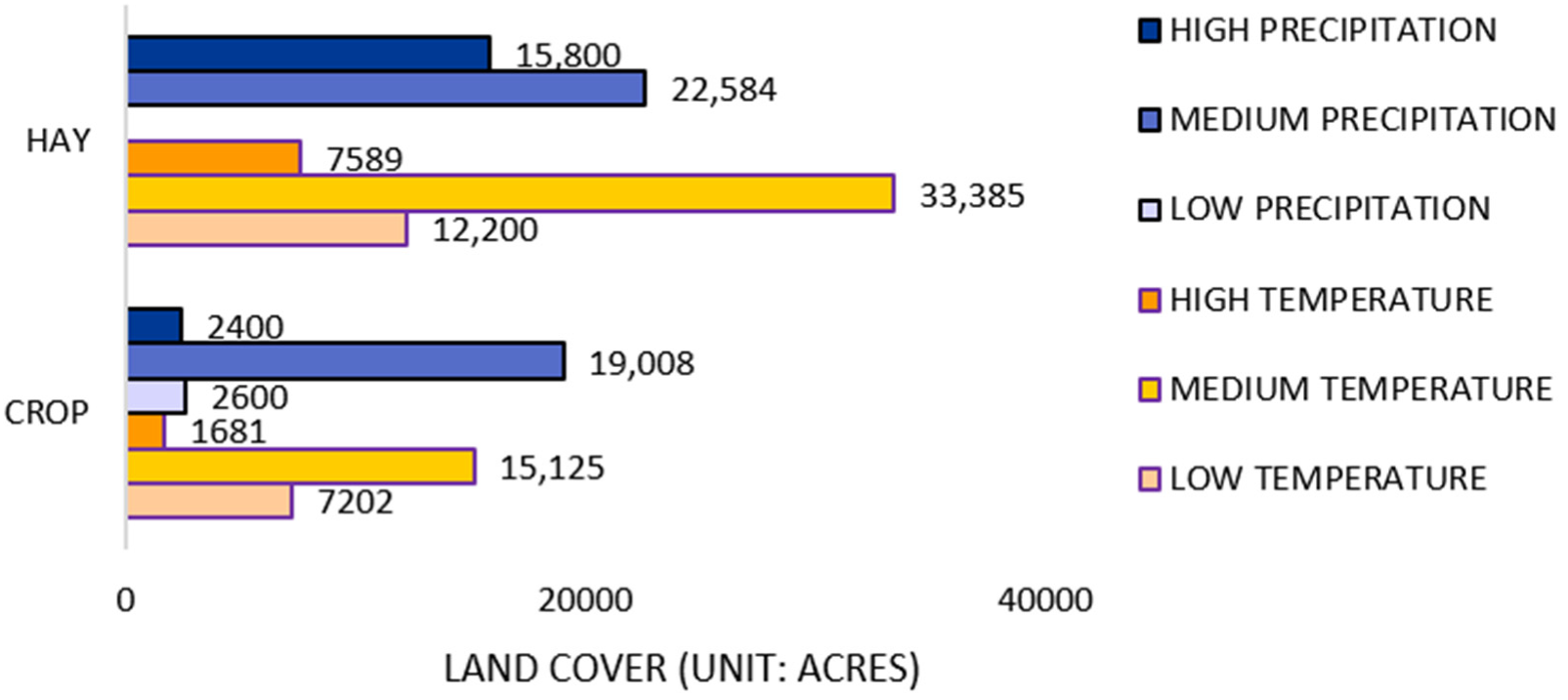
• Relation of land use with food desert indictors. In this stage, the precipitation map is overlaid with the CDL land cover map of Guilford County to study the correlations between them. The land coverage area of fruit, vegetables, row crops, and hay in the study area is calculated considering the magnitude of precipitation from place to place. The same procedure was followed to study the correlation between land use and the temperature, soil quality, and slope of the study area.

3.4. Model Development

In this study, land-use and land-cover change is made by considering the following factors as described in Figure 5: (i) household agents, (ii) land covers, (iii) seasonal fruit and vegetable needs, (iv) land-use related policy, (v) climate variability (temperature and precipitation), (vi) soil quality, and (vii) population growth rate.

Figure 5 shows the overall process for each season to increase the crop production outputs of the county. The data inputs include household data and a land parcel map. In addition, other time-series data, such as the reclassified CDL land-cover map, temperature and precipitation data, soil quality data, and population growth rate data from 2011 to 2020, were used as input for data processing.

To run the simulation, first, the fruit and vegetable needs of the study area are calculated using the CDC daily individual fruit and vegetable intake recommendation based on age and gender. Next, the available farmland size of the county is calculated using the land parcel map. Then, the total land size needed to grow fruits and vegetables to meet the crop requirements of the county is estimated. Finally, land cover changes are made by considering the availability of fruits, vegetables, and fallow lands in the county and the county’s total population, including the future population growth in each season. Note that the land cover changes are made by considering the county’s climate variability and soil quality in each season. This is done by estimating the crop’s production yield that can be obtained in different conditions. For example, in the condition when the quality of farmland soil, rainfall, and temperature availability is suitable or not suitable for farming, the amount of crop yields obtained per acre of land will be different. In other words, crop yields can be increased with high soil quality, sufficient temperature, and rainfall availability. Therefore, the crop yield per acre of farmland was calculated by considering this situation.

• Households. This study used household information to estimate the total food requirement of a specific area since individual daily fruit and vegetable needs depend on them. In the ABM, one household is represented by one agent. It can follow specific rules and make land-use and other decisions based on household-specific data. The food requirement of the community is based on each individual’s needs in the household. During each season time step of the model, farming households went through resource allocation, planting, and harvesting processes. The ABM model runs through 20 farming seasons from 2019 to 2030.
• Farmlands This study used available farmlands in Guilford County for ABM development. In the ABM, one patch of farmland is represented by an agent. This agent follows specific rules and interacts with other agents such as households. The research estimated the county’s annual fruit and vegetable productions from 2011 through 2020 to better understand the correlation between healthy food production and food desert areas in the study area. The production increase or land-use transition recommendation for the future years can be made by considering the county’s population, population growth rate, and the availability of land.
• Seasonal fruit and vegetable needs. Individuals’ daily fruit and vegetable needs vary by age and gender. Adults should consume from 1.5 to 2 cups equivalents of fruits and from 2 to 3 cup-equivalents of vegetables daily, according to the 2020–2025 Dietary Guidelines for Americans. The prevalence of meeting fruit intake recommendations was highest among adults aged ≥51 years (12.5%) and lowest among those living below or close to the poverty level (income to poverty ratio [IPR] < 1.25) (6.8%) (https://www.cdc.gov/mmwr/volumes/71/wr/mm7101a1.htm#suggestedcitation (accessed on 7 January 2022)). Only 9% and 12% of adults ate the recommended amount of vegetables and fruit, respectively, according to a CDC analysis of data from the 2015 Behavioral Risk Factor Surveillance System (https://www.cdc.gov/nccdphp/dnpao/division-information/media-tools/adults-fruits-vegetables.html (accessed on 16 February 2021)). The total daily fruit and vegetable intake is calculated using individuals’ age and gender information based on CDC daily fruit and vegetable intake recommendations at the start of a farming season. This study assumed that people eat fruits and vegetables five days a week; thus, the individual yearly needs are calculated based on Equation (4). This allowed us to estimate the size of land parcels needed to meet the fruit and vegetable requirements.

  $$Yearly crop needs={\displaystyle {\displaystyle \sum }_{n=1}^{\infty }}\left(daily indvidal need{s}_n\right)\times 240$$

  (4)

  Note that this study hypothesizes increasing fruit and vegetable production can minimize the issue of a food desert mainly if local farmers use their fruits and vegetable production to meet their family food needs and locally sell them. Therefore, we have not included the food import or export in the estimations.
• Land-use policies. Federal and state land-use-related policies have a significant impact on crop production. In addition, environmental effects and demands for other outputs (e.g., hay, trees, cash crops, etc.) significantly impact land use changes and crop production. For example, the conversion of forest land into farmland can lead to ecological effects (e.g., effects on the quality of water and wildlife habitat) and socioeconomic effects (e.g., reduction of forest recreation opportunities, reduction of long-term timber production, and loss of open space) as significant implications of forest loss [58]. In addition, farmers may not be interested in using their cash crops, hay, or other land parcels to plant fruits and vegetables for personal use. Instead, they grow cash crops for sale [59] and use their profit to pay their taxes and hire agricultural laborers. In this study, vegetation and wetlands are not recommended to convert to croplands. Based on that context, the land transition in this study is completed to meet the fruit and vegetable requirements of the county from fallow or/and hay lands to fruit or/and vegetable lands.
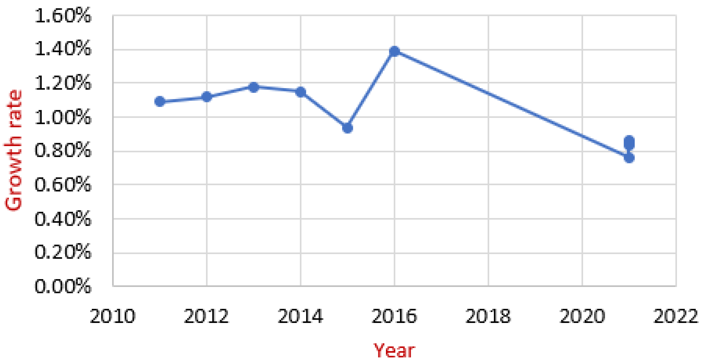
• Population growth rate. Population growth is one of the factors that can drive up demand for food, which typically requires land-use transition to meet the needs. Increases in land dedicated to agricultural purposes may help meet the food demand increased due to population growth. Figure 6 shows the population growth rate of Guilford County from 2011 to 2020. The population growth rate data is used in this study to calculate the seasonal fruit and vegetable needs of Guilford County for each season (Figure 6).
• Climate variability and soil quality. Climate change and soil quality degradation are ongoing problems growing exponentially over the globe as the composition of the atmosphere changes. In North Carolina, the climate has shifted; as a result, the average temperature has increased, and droughts and floods have become more frequent. The production of crops and other agricultural products is impacted by the increasing temperature, precipitation shortage, and soil quality degradation. Depending on the crop types, an increase in average temperature and precipitation may help to increase agricultural production. However, extreme temperatures and precipitation can prevent crops from growing. Therefore, the optimum temperature and precipitation need to be identified for the study area to know their impacts on crop production in the simulation model. The optimum temperature is a temperature suitable for producing crops. Therefore, investigating the relationship between crop yield and climate variability (mainly temperature and precipitation) is essential for predicting agricultural land-use decisions with climate change to understand its impacts on crop yields. Once the county’s seasonal fruit and vegetable requirements for each season are known, the size of farmlands needed to fulfill the vegetable and fruit requirements has to be calculated for each season in terms of suitable temperature, precipitation, and soil quality. For example, suppose the existing fruit and vegetable lands are insufficient to grow the required fruits and vegetables. The model transforms the land cover from fallow and hay to fruits and vegetables in that case. Land-use transition decisions are made by the rainfall, temperature availability, and soil quality of the area. For example, when there is enough rainfall and temperature in the season, the model assumes households can plant and harvest effectively and get more productional outputs since the agricultural production outputs depend on their availability and soil quality. On the other hand, if the season with temperature or rainfall is not optimum (too high or too low), the fruit and vegetable yield will be low, and more land will be involved in the transition to meet the crop requirements of the season. Therefore, the land size to meet the yearly food needs in the county depends on the climate conditions (temperature, rainfall), soil quality, and the population growth rate.
• Crop yield. Once the impacts of climate variability and soil quality are known, the study area’s fruit and vegetable yields are estimated for each season. Crop yield is the main component used in determining overall production and supply. Crop yield is defined as the standard measurement of the amount of agricultural output obtained per unit of land area. One of the standard units of yield measurement is tons per acre in the United States. The average crop yield is estimated using the following formula:

  $$Average crop yield={\displaystyle {\displaystyle \sum }_{i=0}^n}\left(Ln\times \frac{lb}{acer}\times K\right)\times \mathrm{10,000}$$

  (5)

  where Ln is the number of available patch lands in Guilford County, K represents the parameter for precipitation, temperature, and soil quality impacts on crop yields. The value of 10,000 is the average estimated crop yield in pounds (lb) per acre of land [60,61]. Finally, the total land size needs to meet the fruit and vegetable requirements of the county for each season calculated by dividing the yearly crop needs of the county by crop yields per 1 acre of land estimation value.

  $$Total land needs={\displaystyle {\displaystyle \sum }_{i=0}^n}\left(\frac{yearly crop needs}{crop yeilds per 1 acer of land}\right)$$

  (6)

Overall, land cover transitions (e.g., from fallow to farmlands) are done if the available fruit and vegetable lands do not meet the requirements.

4. Results and Discussions

4.1. Model Development

4.1.1. Land Use Relation with Land Productivity and Slope

Figure 7a shows the NCCPI values of the study area obtained from the SSURGO. According to SSURGO, soils with the most suitable characteristics for crop production have larger NCCPI values, whereas soils with low crop yield potential have lower NCCPI values [62]. Based on that context, the study reclassified the NCCPI into three classes: (1) low: the soil with the NCCPI value between 0.01 and 0.40; (2) medium: soil with the NCCPI values between 0.41 and 0.70; and (3) high: the optimum NCCPI suitable for crop and hay production (between 0.71 and 1). As shown in Figure 7a, most of the areas in Guilford County have optimum NCCPI values (between 0.71 and 1). Figure 7b shows the slope map of the study created using DEM. The study classified the slope values in the study area into three classes: (1) low: the optimum slope suitable for crop and hay production (between 0% and 12%); (2) medium: the area with slope values between 13% and 25%; and (3) high: the area with a steep slope (greater than 25%). As shown in Figure 7b, most of the areas in Guilford County have optimum slope values (between 0% and 12%).

The CDL land cover and NCCPI maps were combined to build a spatial relationship between the county’s land use and soil productivity. The NCCPI map was overlaid with the Guilford County land cover map to identify the correlation between soil quality and land covers in the study area. In addition, the CDL land cover and slope maps were combined to build a spatial relationship between the land use of the county and the slope. The overlaid results that show the correlation between land use and soil quality and slope are shown in Figure 8. The chart’s Y-axis represents the type of land coverage: crop and hay, whereas the chart’s X-axis shows the size of crop and hay land coverage in acres. The colors indicate the low, medium, and high values of NCCPI and slopes on the X-axis. For example, the low, medium, and high soil quality values are represented with red colors, as shown in the legend in Figure 8. The medium NCCPI values area is the optimum soil for producing crops and hay. On the other hand, the low, medium, and high values of slopes are represented with red colors. The area with low slope values is the optimum slope for crop and hay production.

As shown in Figure 8 (green colors), 20,143 acres of crops are in the area with optimum soil quality (NCCPI values between 0.7 and 1) compared to 3840 acres and 25 acres in the area with medium and low NCCPI values, respectively. The same trends are seen for the hay land coverage. About 75% (40,575 acres) of hay land coverage is in the area with optimum soil quality. These showed that most of the crop and hay productions of the county are in the area with high NCCPI values.

In addition to soil quality, the slope gradient is crucial for crop and hay production because it influences the runoff flow on the soil surface and the propensity to erodes the soil. As shown in Figure 8 (red colors), more than 80% (20,588 acres) of the crop coverage is in the area with a low or optimum slope percentage (between 0% and 12%). As expected, when the slope values increase, the crop coverage area decreases. The same trends are seen for the hay land cover; about 90% of the hay is in the area with optimum slope. Similar to the crops, the hay coverage area decreases when the slope values are increased in Guilford County.

4.1.2. Land Use Relation with Climate Variability

Figure 9a shows the average annual temperature map of Guilford County from 2011 to 2020 created in this study. The CDL land cover and temperature maps were combined to build a spatial relationship between the county’s land use and temperature. The temperature map was reclassified and overlaid with the Guilford County land cover map to identify the correlation between temperature and land covers. The overlaid results that show the correlation between temperature and land covers are shown in Figure 10. Cool-season crops (such as oats, rye, wheat, and barley) have temperatures: in the range of 32 °F to 41 °F, and warm-season crops (such as tomato, watermelon, pumpkin, and sweet potato) have an optimum temperature between 77 °F to 88 °F [63]. Cool-season crops grow best in cold wintertime weather, whereas warm-season crops are crops that grow better in the hot summertime. Most of the crops in the study area are produced in the warm season (Feb to Oct). Therefore, the study used the average optimum range of temperature, considering the amount of crop production in each season (warm or cool seasons) throughout the year. Based on that context, the temperature map is classified into three groups: (1) low: the area with a temperature value below the optimum temperature for crop and hay production (54 °F–60 °F); (2) medium (optimum): the area with an optimum temperature for crop and hay production (61 °F and 66 °F); and (3) high temperature: the area with a temperature above the optimal value (>67 °F).

Figure 9b shows the average annual rainfall map of Guilford County from 2011 to 2020 created in this study. The CDL land cover and precipitation maps were combined to build a spatial relationship between the county’s land use and land precipitation. The study used the average optimum range of precipitation, considering the amount of crop production in each season (warm or cool seasons) throughout the year [64]. Based on that context, the precipitation map is classified into three groups: (1) low: the area in which precipitation is below the optimum (between 1098 mm and 1200 mm); (2) medium (optimum): the area which receives precipitation between 1201 mm and 1400 mm; and (3) high: the area which receives precipitation of above 1400. Like the temperature map, the precipitation map was overlaid with the Guilford County land cover map to identify the correlation between precipitation and land covers.

The quantitative results in Figure 10 show that the area’s crop coverages with an optimal average yearly temperature (between 61 °F and 66 °F) were 15,125 acres, compared to 1681 and 7202 acres of low- and high-temperature classes, respectively. This shows that relatively more crop production in Guilford County was in the area which received medium (optimum) temperature from 2011 to 2020. The same trends are seen in hay production in Guilford County; about 70% of hay coverage is in the area with optimum temperatures. The quantitative results also show that more than 90% of crop (including fruit, vegetable, and cash crop) coverages were in the area which received medium (optimal) average annual precipitation (between 1200 mm and 1400 mm). This shows that relatively more crop production in Guilford County was in the area which received higher precipitation from 2011 to 2020. The same trends are seen in hay production in Guilford County.

4.2. Simulation Results

This section presents the ABM development outputs for the study area. Figure 11 shows the reclassified land-cover map results of Guilford County for the sample years of 2019 and 2020. The study created reclassified land cover maps from 2011 to 2020 for ABM development purposes, but we presented land cover maps for the 2019 and 2020 seasons as a sample here (Figure 11). As shown in Figure 11, most parts of the county are covered by forest (green colored pixels) and barren lands (brown colored pixels). Moreover, the fruit and vegetable cover of the county is less than 5% compared to other covers.

Figure 12 shows the County’s past fruit and vegetable cover in 2019 and 2020, which this study analyzes from the CDL land cover map. Among the eight land cover classes shown in Figure 12, we presented three land cover types: fruit, vegetable, and fallow, since these are our main focus in the mode development. As shown in Figure 12, Guilford’s 2019 fruit and vegetable covers were 3.1 acres and 17 acres of land, respectively, based on 2029 CDL land cover maps. However, its fruit and vegetable cover in 2020 was 6.5 acres and 20 acres of land, respectively. Therefore, more lands were left as fallow in 2019 and 2020 in the county compared to their fruit and vegetable covers. The land left as fallow was 3433 acres in 2019 compared to 2706 acres in 2020.

The study presented the sample ABM of land cover transition results for 2020 (Figure 13). The y-axis of Figure 13 represents the land coverage size in acres, whereas the x-axis represents the land cover types (vegetable, fruit, and fallow). The blue-colored column of the diagram shows the Guilford County 2020 land cover map. In contrast, the orange-colored column represents the Guilford County 2020 land covers simulated in the ABM after the land transitioned to fulfill the county’s food needs.

The developed ABM results showed that the simulated 2020 fruit and vegetable cover changed from the observed 3 acres and 6.5 acres to 3200 acres and 3617 acres, respectively. This is based on the 2020 population’s food needs based on age and gender. The crop yields that account for the factors that affected crop production, such as climate variability and soil quality. The land cover converted from fallow or hay lands to fruits and vegetables to meet the county’s minimum fruit and vegetable requirements. The created model results illustrated a significant variation in the production of fruits and vegetables over time. One of the reasons for this is the population growth rate of the county and the available farmlands needed to meet the food requirements. There is an average of 1.2% population growth in Guilford County; as a result, fruit and vegetable needs are grown each year. As we see from the results, the land use transition increased the fruit and vegetable cover of the county dramatically. This can enable the local community to have fresh and healthy fruit and vegetables if they buy from the local farmers. In addition, accessing healthy foods from local markets can improve the health of each individual in the community, as not eating enough fruits and vegetables causes chronic diseases. Increasing the amount of land used for farming is one of among the several ways to increase the production of fruits and vegetables at the national and global levels. Our results indicated that the crop transition toward the desired level of fruits and vegetables can still take place within the county, considering the amount of each crop needs, the soil quality, population growth rate, climate variability, and land-use and crop production-related policies. Policies are important. For example, policies may not allow transitioning from forest to farmland, because converting forests into farmland has a negative impact on the ecosystem and has been shown to decrease biodiversity. In addition to land conversion, crop production can be increased on existing farms through intensification, such as using additional fertilizer, machinery, and labor.

The crop production estimated for the area analyzed in the ABM are presented in Figure 14. We used the model’s estimated yield fruit and vegetable outputs. The y-axis of Figure 14 represents the crop production size in tons, whereas the x-axis represents the existing crop yield and the ABM crop yield obtained after the land transition is done. The blue-colored column of the diagram represents the fruit production of the county, whereas the orange-colored column represents the vegetable production of the county.

As we see in Figure 14, the 2020 Guilford County fruit and vegetable productions were 23 tons and 49 tons, respectively. However, the ABM simulation results show that 24,000 tons and 27,128 tons of fruits and vegetables need to meet the food needs. The land transition to meet the food requirement was done from fallow and hay lands to fruit and vegetable. The study assumes producing more fruits and vegetables in the county may minimize the issue of a food desert. For example, farmers and people who do home gardening can have more access to fruit and vegetables than those who buy these foods to eat. In other words, the more fruit and vegetable production in the area, the more people who live in the area can easily access them. Overall, the ABM created in this study can show the uncertainty in production and consumer decision-making processes. For example, at runtime, a range of visual display outputs could be presented in the model, such as land-use change size assigned for fruits and vegetables each season, the changes in land size from one type to another, and the agricultural production outputs in each season.

5. Conclusions

Climate change, urbanization, distribution gaps, income inequality, and population growth pose a considerable threat to global food security, potentially leading to a community food desert. Rainfall and temperature have been identified as two significant factors creating impacts on agricultural productivity. The effective use of farmland and the protection of soils would also contribute substantially to generating equitable and healthy agricultural outcomes. Many scholars have studied the interrelationships between farmers’ decisions, climate variations, and mitigations to achieve sustainable goals as identified by the United Nations (https://www.un.org/en/food-systems-summit (accessed on 23 September 2021)). Studying the interrelationships between factors that cause food insecurity, such as climate variability and land use, will further improve our understanding of food security and help responsible agencies and policymakers plan accordingly to design and implement proper land-use policies. This article introduced a novel approach using an agent-based model of land-use transition to simulate the interactions of the human and environmental systems leading to sufficient fruit and vegetable production.

The approach presented in this article required an iterative development process with several phases. In this study, land-use and land-cover change is modeled by considering the following factors: (i) household agents, (ii) land patches, (iii) seasonal fruit and vegetable needs, (iv) land-use related policy, (v) climate variability (temperature and precipitation), (vi) soil quality, and (vii) population growth rate. The data used for developing the model included: Parcel land polygons, annual rainfall, temperature data, CDL, and annual precipitations and temperature data. The model result showed that the 2020 fruit and vegetable covers changed from the CDL 3 acres and 6.5 acres covers to 3200 acres and 3617 acres, respectively, to fulfill the fruit and vegetable needs of the county. The simulation results reported are based on the 2020 population’s food needs considering individuals’ age and gender. However, acquiring sufficient data to validate the outcomes is the main challenge of this study. For example, information regarding each individual’s fruit and vegetable purchases from the local farmer in our study area were not available and we used state average estimates instead. The study used CDL land covers of the study area as a point of reference to learn about previous fruit and vegetable covers as well as crop yields, which could be likewise improved with more detailed data. Many other assumptions had to be made in the proposed system research, for example, the timeframe of the data acquired, consistent production and consumption patterns, and steady weather conditions.

The proposed model explores alternative scenarios to improve livelihoods and mitigate the impact of land use, climate variability, soil quality, and population growth related to accessing fresh fruits and vegetables. Our approach can be used as a tool for stakeholders, policymakers, and other responsible agencies to ensure all the community residents obtain fresh and affordable fruits and vegetables through a sustainable food system.

References

- Brown, C.; Miller, S. The Impacts of Local Markets: A Review of Research on Farmers Markets and Community Supported Agriculture (CSA). Am. J. Agric. Econ. 2008, 90, 1296–1302. [Google Scholar] [CrossRef]
- Onyango, B.M.; Hallman, W.K.; Bellows, A.C. Purchasing organic food in U.S. food systems: A study of attitudes and practice. Br. Food J. 2007, 109, 399–411. [Google Scholar] [CrossRef] [Green Version]
- Schnell, S.M. Food with a ffarmer’sface: Community-supported agriculture in the United States. Geogr. Rev. 2007, 97, 550–564. [Google Scholar] [CrossRef]
- Bentsen, K.; Pedersen, P.E. Consumers in local food markets: From adoption to market co-creation? Br. Food J. 2020, 123, 1083–1102. [Google Scholar] [CrossRef]
- Liang, C.-L.; Kurkalova, L.; Beni, L.H.; Mulrooney, T.; Jha, M.; Miao, H.; Monty, G. Introducing an innovative design to examine human-environment dynamics of food deserts responding to COVID-19. J. Agric. Food Syst. Community Dev. 2021, 10, 123–133. [Google Scholar] [CrossRef]
- Lele, U.; Klousia-Marquis, M.; Goswami, S. Good Governance for Food, Water and Energy Security. Aquat. Procedia 2013, 1, 44–63. [Google Scholar] [CrossRef]
- Termeer, C.J.; Drimie, S.; Ingram, J.; Pereira, L.; Whittingham, M.J. A diagnostic framework for food system governance arrangements: The case of South Africa. NJAS—Wagening. J. Life Sci. 2018, 84, 85–93. [Google Scholar] [CrossRef]
- Hendrickson, D.; Smith, C.; Eikenberry, N. Fruit and vegetable access in four low-income food deserts communities in Minnesota. Agric. Hum. Values 2006, 23, 371–383. [Google Scholar] [CrossRef]
- Bitler, M.; Steven, J.H. An economic view of food deserts in the United States. J. Policy Anal. Manag. 2011, 30, 153–176. [Google Scholar]
- Leschewski, A.M.; Weatherspoon, D.D. Fast food restaurant pricing strategies in Michigan food deserts. Int. Food Agribus. Manag. Rev. 2014, 17, 147–170. [Google Scholar]
- Hake, M.; Engelhard, E.; Dewey, A.; Gundersen, C. The Impact of the Coronavirus on Child Food Insecurity; Feeding America: Chicago, IL, USA, 2020. [Google Scholar]
- Lewis, E.C.; Colón-Ramos, U.; Gittelsohn, J.; Clay, L. Food-seeking behaviors and food insecurity risk during the Coronavirus disease 2019 pandemic. J. Nutr. Educ. Behav. 2022, 54, 159–171. [Google Scholar] [CrossRef]
- Ploeg, M.V.; Dutko, P.; Breneman, V. Measuring Food Access and Food Deserts for Policy Purposes. Appl. Econ. Perspect. Policy 2015, 37, 205–225. [Google Scholar] [CrossRef] [Green Version]
- McGuire, S.; FAO; IFAD; WFP. The state of food insecurity in the world 2015: Meeting the 2015 international hunger targets: Taking stock of uneven progress. Adv. Nutr. 2015, 6, 623–624. [Google Scholar] [CrossRef] [Green Version]
- USDA. Food Security and Nutrition Assistance. 2020. Available online: https://www.ers.usda.gov/data-products/ag-and-food-statistics-charting-the-essentials/food-security-and-nutrition-assistance/?topicId=c40bd422-99d8-4715-93fa-f1f7674be78b (accessed on 24 April 2020).
- Neuhouser, M.L. The importance of healthy dietary patterns in chronic disease prevention. Nutr. Res. 2019, 70, 3–6. [Google Scholar] [CrossRef]
- Kelli, H.M.; Kim, J.H.; Tahhan, A.S.; Liu, C.; Ko, Y.; Hammadah, M.; Sullivan, S.; Sandesara, P.; Alkhoder, A.A.; Choudhary, F.K.; et al. Living in Food Deserts and Adverse Cardiovascular Outcomes in Patients with Cardiovascular Disease. J. Am. Hear. Assoc. 2019, 8, e010694. [Google Scholar] [CrossRef] [Green Version]
- Testa, A.; Jackson, D.B.; Semenza, D.C.; Vaughn, M.G. Food deserts and cardiovascular health among young adults. Public Health Nutr. 2021, 24, 117–124. [Google Scholar] [CrossRef]
- Dubowitz, T.; Ncube, C.; Leuschner, K.; Tharp-Gilliam, S. A natural experiment opportunity in two low-income urban food desert communities: Research design, community engagement methods, and baseline results. Health Educ. Behav. 2015, 42 (Suppl. S1), 87S–96S. [Google Scholar] [CrossRef] [Green Version]
- Ghosh-Dastidar, M.; Hunter, G.; Collins, R.L.; Zenk, S.N.; Cummins, S.; Beckman, R.; Nugroho, A.K.; Sloan, J.C.; Wagner, L.; Dubowitz, T. Does opening a supermarket in a food desert change the food environment? Health Place 2017, 46, 249–256. [Google Scholar] [CrossRef] [PubMed]
- Masipa, T.S. The impact of climate change on food security in South Africa: Current realities and challenges ahead. Jàmbá J. Disaster Risk Stud. 2017, 9, 7. [Google Scholar] [CrossRef] [Green Version]
- Ray, D.K.; Gerber, J.S.; MacDonald, G.K.; West, P.C. Climate variation explains a third of global crop yield variability. Nat. Commun. 2015, 6, 5989. [Google Scholar] [CrossRef] [Green Version]
- Matiu, M.; Ankerst, D.P.; Menzel, A. Interactions between temperature and drought in global and regional crop yield variability during 1961–2014. PLoS ONE 2017, 12, e0178339. [Google Scholar] [CrossRef] [PubMed] [Green Version]
- George, D.R.; Kraschnewski, J.L.; Rovniak, L.S. Public health potential of farmers’ markets on medical center campuses: A case study from Penn State Milton S. Hershey Medical Center. Am. J. Public Health 2011, 101, 2226–2232. [Google Scholar] [CrossRef] [PubMed]
- Rimal, B.; Zhang, L.; Keshtkar, H.; Wang, N.; Lin, Y. Monitoring and Modeling of Spatiotemporal Urban Expansion and Land-Use/Land-Cover Change Using Integrated Markov Chain Cellular Automata Model. ISPRS Int. J. Geo-Inf. 2017, 6, 288. [Google Scholar] [CrossRef] [Green Version]
- Azubike, C.S.; Kurkalova, L.A.; Mulrooney, T.J. Modeling Land Use and Land Cover in North Carolina; a Markov Chain Approach. In Proceedings of the 2019 Annual Meeting, Atlanta, GA, USA, 21–23 July 2019. [Google Scholar]
- Liu, X.; Liang, X.; Li, X.; Xu, X.; Ou, J.; Chen, Y.; Li, S.; Wang, S.; Pei, F. A future land use simulation model (FLUS) for simulating multiple land use scenarios by coupling human and natural effects. Landsc. Urban Plan. 2017, 168, 94–116. [Google Scholar] [CrossRef]
- Lambin, E.F.; Geist, H.J.; Lepers, E. Dynamics of Land-Use and Land-Cover Change in Tropical Regions. Annu. Rev. Environ. Resour. 2003, 28, 205–241. [Google Scholar] [CrossRef] [Green Version]
- Jiao, W.; Zhang, L.; Chang, Q.; Fu, D.; Cen, Y.; Tong, Q. Evaluating an Enhanced Vegetation Condition Index (VCI) Based on VIUPD for Drought Monitoring in the Continental United States. Remote Sens. 2016, 8, 224. [Google Scholar] [CrossRef] [Green Version]
- Rahman, S.; Di, L.; Yu, E.; Lin, L.; Yu, Z. Remote Sensing Based Rapid Assessment of Flood Crop Damage Using Novel Disaster Vegetation Damage Index (DVDI). Int. J. Disaster Risk Sci. 2021, 12, 90–110. [Google Scholar] [CrossRef]
- Zhang, R.; Tang, C.; Ma, S.; Yuan, H.; Gao, L.; Fan, W. Using Markov chains to analyze changes in wetland trends in arid Yinchuan Plain, China. Math. Comput. Model. 2011, 54, 924–930. [Google Scholar] [CrossRef]
- Ding, Z.; Gong, W.; Li, S.; Wu, Z. System dynamics versus agent-based modeling: A review of complexity simulation in construction waste management. Sustainability 2018, 10, 2484. [Google Scholar] [CrossRef] [Green Version]
- Zhu, Y.; Diao, M.; Ferreira, J.; Zegras, C. An integrated microsimulation approach to land-use and mobility modeling. J. Transp. Land Use 2018, 11, 633–659. [Google Scholar] [CrossRef]
- Verburg, P.H.; Alexander, P.; Evans, T.; Magliocca, N.R.; Malek, Z.; DA Rounsevell, M.; van Vliet, J. Beyond land cover change: Towards a new generation of land use models. Curr. Opin. Environ. Sustain. 2019, 38, 77–85. [Google Scholar] [CrossRef]
- Dadhich, P.N.; Hanaoka, S. Remote sensing, GIS and MMarkov’smethod for land use change detection and prediction of Jaipur district. J. Geomat. 2010, 4, 9–15. [Google Scholar]
- Sang, L.; Zhang, C.; Yang, J.; Zhu, D.; Yun, W. Simulation of land use spatial pattern of towns and villages based on CA—Markov model. Math. Comput. Model. 2011, 54, 938–943. [Google Scholar] [CrossRef]
- El-Hallaq, M.A.; Habboub, M.O. Using cellular automata-Markov analysis and multi criteria evaluation for predicting the shape of the Dead Sea. Adv. Remote Sens. 2015, 4, 83. [Google Scholar] [CrossRef] [Green Version]
- Moeckel, R.; Schürmann, C.; Wegener, M. Microsimulation of urban land use. In Proceedings of the 42nd European Congress of the Regional Science Association, Dortmund, Germany, 27–31 August 2002; pp. 27–31. [Google Scholar]
- Natalini, D.; Bravo, G.; Jones, A.W. Global food security and food riots—An agent-based modelling approach. Food Secur. 2019, 11, 1153–1173. [Google Scholar] [CrossRef]
- Namany, S.; Govindan, R.; Al-Fagih, L.; McKay, G.; Al-Ansari, T. Sustainable food security decision-making: An agent-based modelling approach. J. Clean. Prod. 2020, 255, 120296. [Google Scholar] [CrossRef]
- Wossen, T.; Berger, T. Climate variability, food security and poverty: Agent-based assessment of policy options for farm households in Northern Ghana. Environ. Sci. Policy 2015, 47, 95–107. [Google Scholar] [CrossRef]
- Alghais, N.; Pullar, D. Modelling future impacts of urban development in Kuwait with the use of ABM and GIS. Trans. GIS 2018, 22, 20–42. [Google Scholar] [CrossRef]
- Rounsevell, M.D.; Pedroli, B.; Erb, K.-H.; Gramberger, M.; Busck, A.G.; Haberl, H.; Kristensen, S.; Kuemmerle, T.; Lavorel, S.; Lindner, M.; et al. Challenges for land system science. Land Use Policy 2012, 29, 899–910. [Google Scholar] [CrossRef]
- Huber, R.; Bakker, M.; Balmann, A.; Berger, T.; Bithell, M.; Brown, C.; Grêt-Regamey, A.; Xiong, H.; Le, Q.B.; Mack, G.; et al. Representation of decision-making in European agricultural agent-based models. Agric. Syst. 2018, 167, 143–160. [Google Scholar] [CrossRef] [Green Version]
- Heckbert, S.; Baynes, T.; Reeson, A. Agent-based modeling in ecological economics. Ann. N. Y. Acad. Sci. 2010, 1185, 39–53. [Google Scholar] [CrossRef] [PubMed]
- Sun, Z.; Lorscheid, I.; Millington, J.D.; Lauf, S.; Magliocca, N.R.; Groeneveld, J.; Balbi, S.; Nolzen, H.; Müller, B.; Schulze, J.; et al. Simple or complicated agent-based models? A complicated issue. Environ. Model. Softw. 2016, 86, 56–67. [Google Scholar] [CrossRef] [Green Version]
- Dai, E.; Ma, L.; Yang, W.; Wang, Y.; Yin, L.; Tong, M. Agent-based model of land system: Theory, application and modelling framework. J. Geogr. Sci. 2020, 30, 1555–1570. [Google Scholar] [CrossRef]
- Auchincloss, A.H.; Garcia, L.M.T. Brief introductory guide to agent-based modeling and an illustration from urban health research. Cad. Saude Publica 2015, 31, 65–78. [Google Scholar] [CrossRef] [PubMed] [Green Version]
- Gebrehiwot, A.; Beni, L.H.; Kurkalova, L.A.; Liang, C.L.; Jha, M.K.; Mulrooney, T.J.; Dhamankar, S. Agent Based Modeling of Land Use and Land Cover Changes to Assess Community Food Desert Using Geospatial Technology. In Proceedings of the AGU Fall Meeting 2021, New Orleans, LA, USA, 13–17 December 2021. [Google Scholar]
- Dhamankar, S.; Beni, L.H.; Kurkalova, L.A.; Jha, M.K.; Liang, C.L.; Mulrooney, T.J.; Monty, G.; Gebrehiwot, A. Geospatial Data Analysis to Understand Food Security. In Proceedings of the AGU Fall Meeting 2021, New Orleans, LA, USA, 13–17 December 2021. [Google Scholar]
- Demir, Z.; Tursun, N.; Işık, D. Effects of different cover crops on soil quality parameters and yield in an apricot orchard. Int. J. Agric. Biol. 2019, 21, 399–408. [Google Scholar]
- Goudie, A.S. Human Impact on the Natural Environment, 8th ed.; John Wiley & Sons: Hoboken, NJ, USA, 2018. [Google Scholar]
- Guan, C.; Rowe, P.G. Should big cities grow? Scenario-based cellular automata urban growth modeling and policy applications. J. Urban Manag. 2016, 5, 65–78. [Google Scholar] [CrossRef]
- Mulrooney, T.; Foster, R.; Jha, M.; Beni, L.H.; Kurkalova, L.; Liang, C.L.; Miao, H.; Monty, G. Using geospatial networking tools to optimize source locations as applied to the study of food availability: A study in Guilford County, North Carolina. Appl. Geogr. 2021, 128, 102415. [Google Scholar] [CrossRef]
- Baumhardt, R.L.; Stewart, B.A.; Sainju, U.M. North American Soil Degradation: Processes, Practices, and Mitigating Strategies. Sustainability 2015, 7, 2936–2960. [Google Scholar] [CrossRef] [Green Version]
- Smith, G.; Archer, R.; Nandwani, D.; Li, J. Impacts of urbanization: Diversity and the symbiotic relationships of rural, urban, and spaces in-between. Int. J. Sustain. Dev. World Ecol. 2018, 25, 276–289. [Google Scholar] [CrossRef]
- Kurkalova, L.A.; Beni, L.H.; Liang, C.-L. Vegetable production: Land use perspective. In Proceedings of the Elected Poster: AAEA Annual Meeting, Austin, TX, USA, 1–3 August 2021. [Google Scholar]
- Kim, T.J.; Wear, D.N.; Coulston, J.; Li, R. Forest land use responses to wood product markets. For. Policy Econ. 2018, 93, 45–52. [Google Scholar] [CrossRef]
- Schneider, K.; Gugerty, M.K. The impact of export-driven cash crops on smallholder households. Gates Open Res. 2019, 3, 1379. [Google Scholar]
- Schreinemachers, P. The (Ir) Relevance of the Crop Yield Gap Concept to Food Security in Developing Countries; Cuvillier Verlag: Göttingen, Germany, 2006. [Google Scholar]
- Juma, G.S.; Beru, F.K. Prediction of Crop Yields under a Changing Climate. In Agrometeorology; BoD—Books on Demand: Norderstedt, Germany, 2021. [Google Scholar]
- Bandaru, V.; Izaurralde, R.; Manowitz, D.; Link, R.; Zhang, X.; Post, W.M. Soil Carbon Change and Net Energy Associated with Biofuel Production on Marginal Lands: A Regional Modeling Perspective. J. Environ. Qual. 2013, 42, 1802–1814. [Google Scholar] [CrossRef]
- Ralph, E.N. Growing Season Characteristics and Requirements in the Corn Belt; Purdue University: West Lafayette, IN, USA, 2019; Available online: https://mdc.itap.purdue.edu/item.asp?itemID=20092 (accessed on 23 May 1990).
- Ritchie, I. Precipitation Impact on Crop Yield. Bachelor’s Thesis, University of Nebraska-Lincoln, Lincoln, NE, USA, 2021. [Google Scholar]
Publisher’s Note: MDPI stays neutral with regard to jurisdictional claims in published maps and institutional affiliations. |
© 2022 by the authors. Licensee MDPI, Basel, Switzerland. This article is an open access article distributed under the terms and conditions of the Creative Commons Attribution (CC BY) license (https://creativecommons.org/licenses/by/4.0/).
Share and Cite
Gebrehiwot, A.A.; Hashemi-Beni, L.; Kurkalova, L.A.; Liang, C.L.; Jha, M.K. Using ABM to Study the Potential of Land Use Change for Mitigation of Food Deserts. Sustainability 2022, 14, 9715. https://doi.org/10.3390/su14159715
Gebrehiwot AA, Hashemi-Beni L, Kurkalova LA, Liang CL, Jha MK. Using ABM to Study the Potential of Land Use Change for Mitigation of Food Deserts. Sustainability. 2022; 14(15):9715. https://doi.org/10.3390/su14159715
Chicago/Turabian StyleGebrehiwot, Asmamaw A., Leila Hashemi-Beni, Lyubov A. Kurkalova, Chyi L. Liang, and Manoj K. Jha. 2022. "Using ABM to Study the Potential of Land Use Change for Mitigation of Food Deserts" Sustainability 14, no. 15: 9715. https://doi.org/10.3390/su14159715
APA StyleGebrehiwot, A. A., Hashemi-Beni, L., Kurkalova, L. A., Liang, C. L., & Jha, M. K. (2022). Using ABM to Study the Potential of Land Use Change for Mitigation of Food Deserts. Sustainability, 14(15), 9715. https://doi.org/10.3390/su14159715