Abstract
Traditionally, distribution uniformity has been obtained by using rain gauges, which makes it a very expensive process. This paper sought to create a simulation strategy using QGIS and EPANET, both free software, that allowed the simulation of the water application results of all the emitters of an irrigation installation. In this way, it was possible to obtain the geospatial representation of the applied water and finally to know the distribution uniformity in the whole installation. The simulation finally fulfilled its objective and was compared with a study of distribution uniformity with rain gauges. The biggest difference between the measured and simulated data was a difference of 5.76% among the sectors. The simulated uniformity was very similar to the measured uniformity, which allowed us to affirm that the proposed simulation methodology was adequate. We believe that the methodology proposed in this article could be very useful in improving the management of sprinkler irrigation systems, particularly those in which distribution uniformity is of special importance. These improvements in management can also result in savings in water and other inputs, which are becoming increasingly important in the current context of climate change and the reduction in the impact of agriculture on the environment. Finally, similar studies could be carried out with the same tools for other pressurized irrigation systems, such as sprinkler irrigation outside greenhouses and drip irrigation.
1. Introduction
Among all the conditioning factors affecting food production and water supply, irrigation is one of the most important. Worldwide, irrigated agriculture accounts for 20% of total cultivated land and provides 40% of the food produced in the world [1]. The impact of irrigation, however, varies in each region, depending on the conditions of the area and the use of the resources. In the European Union, Spain has the largest irrigated area, covering almost four million hectares, having increased by 14% in less than 20 years [2]. In Spain, 77% of the irrigated area is irrigated by pressurized irrigation, in which sprinkler irrigation is of great importance (14.8% of the irrigated area) [3]. The implementation of irrigation results in a large increase in productivity. Therefore, climate change is expected to favor the introduction of technologies that will improve water use efficiency. Specifically, in the case of developed countries, it is expected that in the near future the irrigated area will increase by 34% and the water used by 14% [4].
The impact of irrigation is therefore enormous, both in terms of the benefit to society in relation to food production and the damage it causes. For example, it is estimated that irrigation accounts for 70% of all freshwater withdrawals worldwide [1]. Therefore, the most important challenge will be to mitigate the negative impacts produced without reducing the benefits generated for society. This means that there is an increasing need to know how irrigation systems are performing in order to make them more effective and efficient. Effectiveness in an irrigation system consists of its capacity to provide the required quantity at the right time and the conditions necessary for the correct development of the plant. As for efficiency, it is the ability to use the available resources in the most productive way possible.
In this sense, when evaluating an irrigation system, distribution uniformity is one of the magnitudes that allows for both conditions to be assessed. The distribution uniformity is the parameter that characterizes the irrigation emitters’ relative distribution of irrigation water on the surface. Knowledge of this value will help characterize the irrigation system as a whole, as it is influenced by factors such as emitter layout, pumping, pipe routing, etc. Studies such as Eng et al. [5] measured distribution uniformity for sprinklers under greenhouse conditions. As long as the needs are uniform over the entire surface, the water application will be the same throughout the field, i.e., maximum uniformity. A distribution uniformity of less than 100% will mean that there will be under- or over-irrigated areas, or both, which will negatively affect the effectiveness and efficiency of the irrigation system.
Emitter manufacturers often provide approximate distribution uniformity data depending on the model, sprinkler arrangement, and operating conditions. However, if reliable data are desired, it is in principle necessary to measure distribution uniformity directly under irrigation conditions. This need is due to the great dependence of the distribution uniformity on variables such as hydraulic pressure at the emitter, wind or topography, and the coefficient of variation of the microirrigation emitters which causes the distribution uniformity to vary significantly and easily, both spatially and temporally. Traditionally, this measurement has been made by placing a network of rain gauges or water collectors on the surface to be studied. The values thus obtained are used to calculate various coefficients that give an idea of the distribution uniformity. Although effective, this methodology is limited by the need for field data, which are often costly to obtain, especially if one wishes to study large areas. For this reason, in recent years, taking advantage of computer technology, models and tools have become available to simulate the behavior of sprinklers under different initial conditions and large surface areas, which in turn allows distribution uniformity to be estimated in an extended manner.
Most modeling studies on sprinkler water distribution have focused on simulating the behavior of a single sprinkler with a few input variables (Playán et al. [6], Li, Bai, and Yan [7] or Zhang, Merkley, and Pinthong [8]). These investigations, however, only simulated uniformity for isolated sprinklers, and did not consider the effect of overlap on distribution uniformity. Other studies such as Chen et al. [9] or Do Prado and Colombo [10] succeeded in simulating distribution uniformity with several moving sprinklers using the commercial programming platform MATLAB, and the commercial program Si-mulasoft, respectively. Fukui, Nakanishi, and Okamura [11] did the same but with stationary sprinklers. Apart from specific studies, commercial software has been developed that allows the distribution uniformity of sprinkler blocks to be known by using hydraulic simulations such as SPACE Pro [12] or SIRIAS [13].
However, the major limitation of the studies shown so far is the lack of spatial generalization of the results and the use of non-free software. These investigations and methodologies work adequately for certain conditions that do not represent, for example, what happens on an extensive farm but are limited to specific areas. Therefore, the main objective of this work was to propose and evaluate a methodology that allows the uniformity of the application of sprinkler irrigation in the whole area occupied by greenhouses on a given farm to be known without the need for direct measurements. The evaluation with field data of the proposed methodology was carried out at the level of irrigation sectors; this was a level of detail that we believed was sufficient at this stage of the study. This main objective required the previous fulfillment of others: (i) the determination of the pressures and flow rates in all the sprinklers of the installation using the free hydraulic simulation software EPANET; (ii) the determination of the distributed rainfall and flow rate curve as a function of pressure for the working sprinklers; (iii) assign to each location the precipitation corresponding to irrigation, which in turn would allow estimating the uniformity of the application, using the interaction between the free GIS program QGIS and EPANET. The uniformity thus obtained was compared with in situ measurements to evaluate the methodology’s validity.
Although this is not the first time that the interaction of both programs has been used, it is the first time it has been used to simulate a system with a pressure-dependent demand. So far, the studies that have integrated both programs have done so for supply networks with fixed flow rates, such as the studies of Pérez-Padillo et al. [14], Muller et al. [15], Safitri et al. [16], Estong et al. [17] and Nagarajan and Charhate [18]. Other studies used GIS and hydraulic simulation programs for flood hazard zoning [19] or used GIS tools to determine shoreline morphological changes [20]. The only study that used a GIS program with EPANET was the EPANET study of Pérez Urrestarazu et al. [21] for failure and problem area monitoring in different irrigation sectors. Therefore, it will be the first time that QGIS and EPANET have been used together to geospatially represent rainfall and calculate distribution uniformity in a system with a pressure-dependent demand.
2. Materials and Methods
2.1. Description of the Hydraulic Systems in the Greenhouses Studied
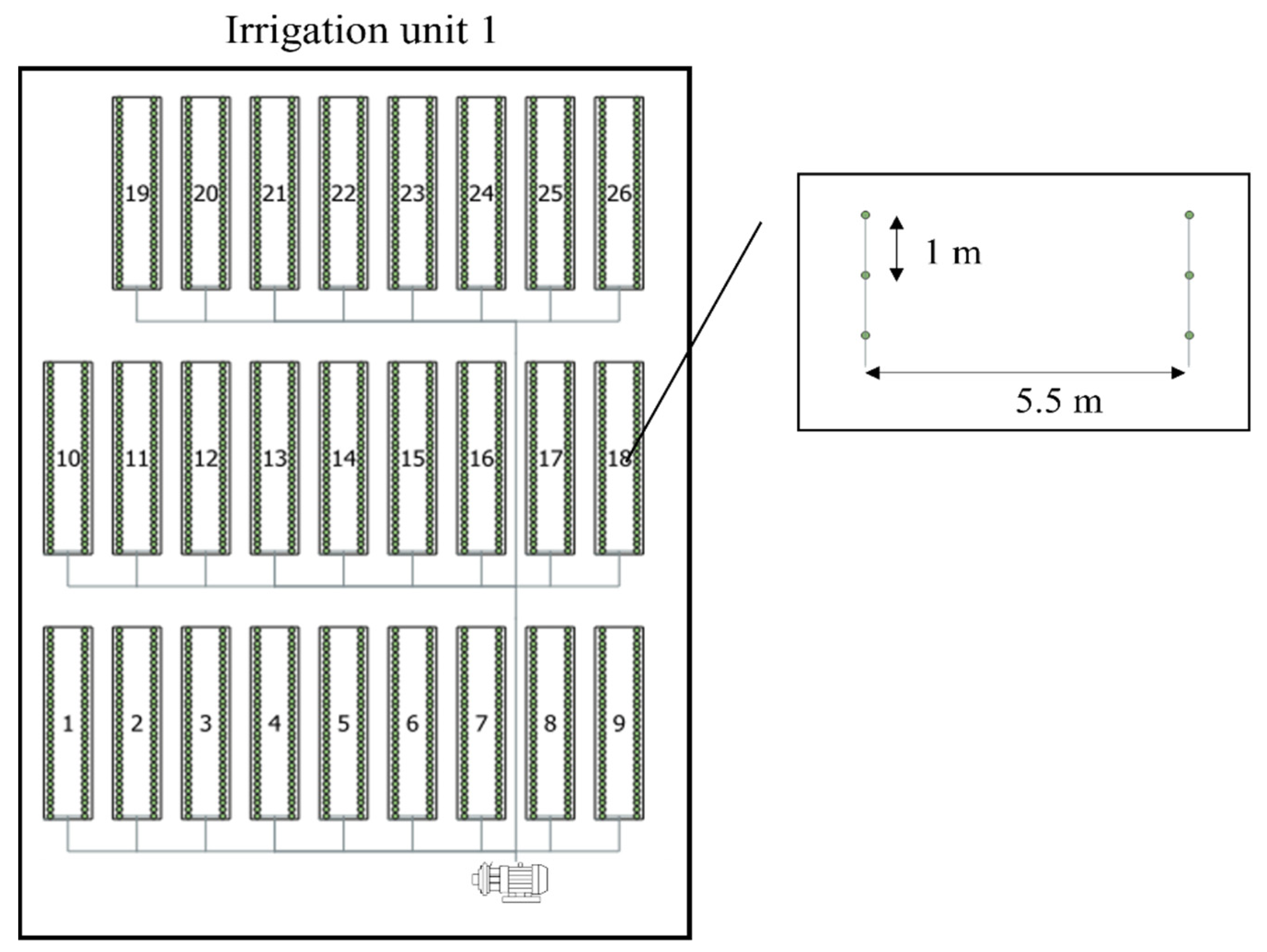
A greenhouse agricultural facility was chosen for this study. The irrigation system was sprinkler irrigation. The sprinklers were located along the length and width of the greenhouses at a height of about 1.8 m above the ground. The agricultural facility had 26 greenhouses. The sectors had an almost flat slope. The irrigation unit was sized to irrigate three irrigation sectors simultaneously. The sprinkler arrangement was 5.5 × 1.0 m with the Green Spin 120 model of NaanDanJain company (Figure 1). The nominal flow rate of the sprinklers was 120 L/h with a nominal pressure of 2 bar. The surface area in each sector was different, varying from 500 m2 to 650 m2. A single vertical centrifugal pump drove the water.
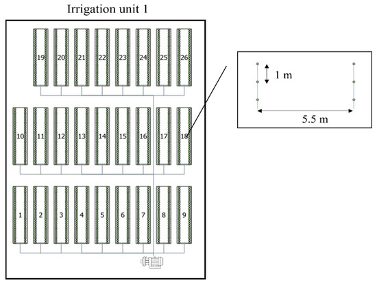
Figure 1.
Diagram of the installations showing the irrigation sectors and sprinkler arrangement.
2.2. In Situ Measurement of Distribution Uniformity
As already discussed, the main objective of this work was to quantify water application in the different areas of an installation by sprinklers to calculate the distribution uniformity. The simulation would allow an estimation of the distribution uniformity without the need to take data in the field. However, a distribution uniformity study with the classical methodology was necessary to evaluate the simulations correctly and to determine if they gave correct results. This way, the simulation results could be compared with those obtained in the study and whether the proposed methodology yielded adequate results could be checked. For this purpose, several rain gauges were placed in sectors 5 and 23, and irrigation was applied for 30 min. In each trial, 24 rain gauges were placed at a frame of 0.5 × 1 m, covering an area of 7 m2 (Figure 2). The dimensions of the catch can array were based on the sector’s width and the sprinklers’ arrangement. While irrigation was in operation, data on the maximum and minimum pressures of the sector in which the study was conducted were obtained manually.
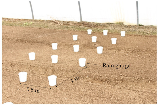
Figure 2.
Rain gauges for distribution uniformity studies.
To obtain the distribution uniformity, for this experiment the Christiansen’s uniformity coefficient proposed by Christiansen (1942) [22] at the University of California (1) was used for this experiment:
where is the amount of water collected by each catch rain gauge (in mm), is the average value collected by the gauges, and n is the total number of rain gauges.
The value obtained from (1) reported the distribution uniformity of the studied area, i.e., 7 m2. To extrapolate this value to that of the sector in which it is being measured, Equation (2) was used that takes into account the pressure differences of the sprinklers in the sector [23]:
where is the uniformity coefficient of the system or sector, CU is the uniformity coefficient of the measurement area., is the minimum pressure in the system and is the average pressure of the system. For this purpose, the maximum and minimum sprinkler pressure was measured in the two sectors where uniformity was measured.
2.3. Sprinkler Evaluation: Flow vs. Pressure Relationship and Depth of Water Application Distribution vs. Pressure
In order to proceed with the simulations, it was necessary to have the flow vs. pressure relationship of the sprinkler, which was the Green Spin 120 model (NaanDanJain) and also the water application distribution vs. pressure. One of the particularities of this simulation was that the sprinkler water supply would depend on the incoming pressure. Therefore, if one wanted to know the water delivery of each sprinkler (“demand”), one would have to know the flow vs. pressure relationship of the sprinkler (Figure 3). The flow vs. pressure relationship was defined by the discharge coefficient and the discharge exponent (3).
where q is the emitter flow rate, k is the discharge coefficient, h is the pressure at the emitter inlet, and x is the discharge exponent.
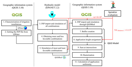
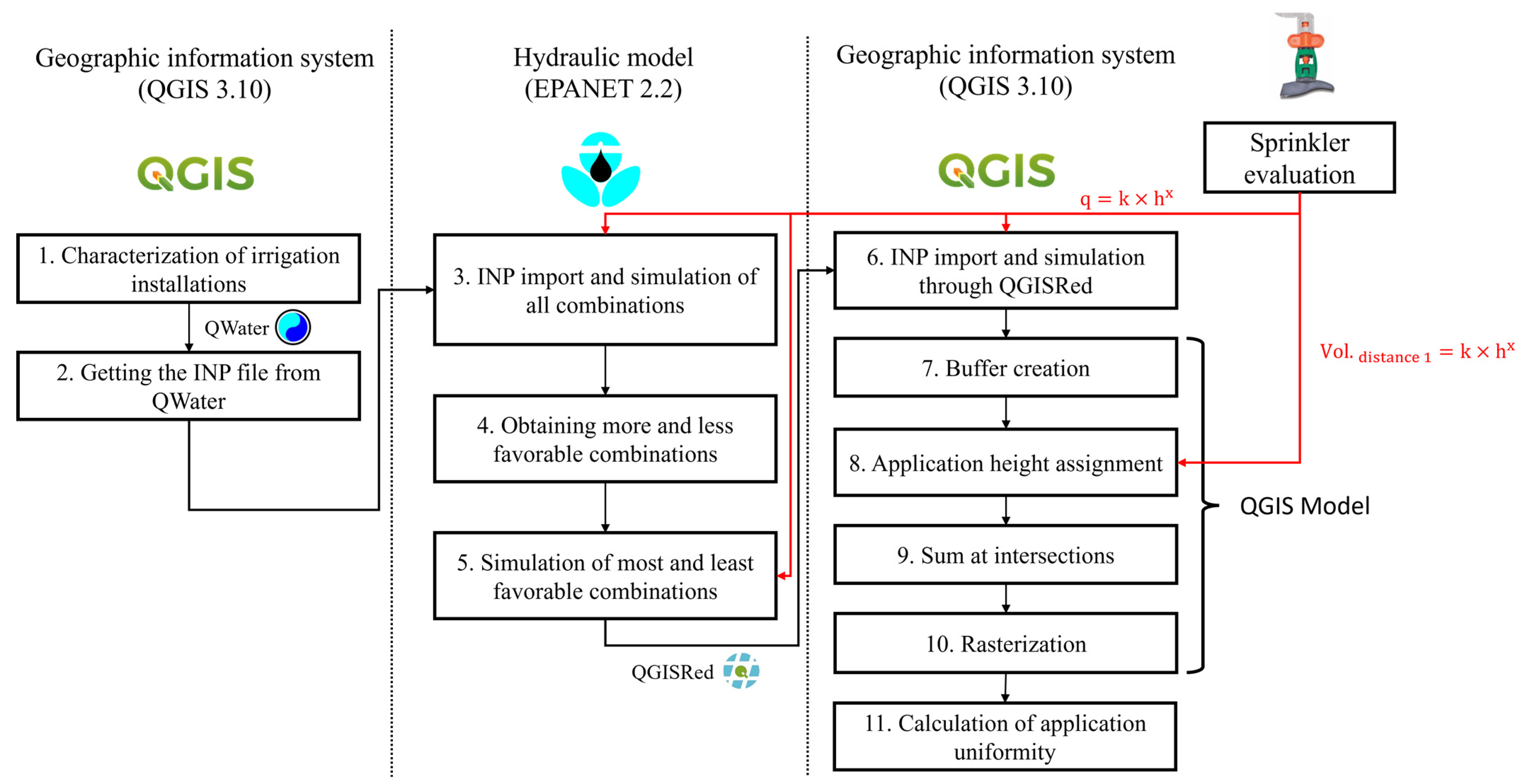
Figure 3.
Interaction of QGIS and EPANET programs for creating a simulation model to determine the distribution uniformity of a facility.
These values were obtained in a hydraulics laboratory by measuring the flow rate at different pressures and performing a geometric regression process.
The discharge coefficient and discharge exponent obtained were as follows (Table 1).

Table 1.
Discharge coefficient and exponent of the used sprinkler model.
Equation (3) reports the total flow delivered depending on the incoming pressure but does not show how it was distributed in the space. Therefore, a sprinkler was placed in the same laboratory at the same height as in the greenhouses, and six rain gauges were placed 0.5 m apart along the same radius of the jet so that they were arranged along the 3 m. The precipitation in each rain gauge was determined at different pressures (1.1 bar and 2.4 bar) and by means of a geometric regression process, the characteristic curve was determined (ec. 4).
where p is the precipitation rate (mm/h) at each sampled distance (d), k and x are fitted parameters at each distance. The characteristic curve was as follows (Table 2).
Table 2.
Values of kd and xd for each sprinkler model and each distance.
Negative values of xd indicate that at higher pressure the application at that distance is lower. Values of zero indicate that the pressure does not affect the water applied at that distance.
2.4. Pressure Simulation
The programs used for rainfall simulation were the QGIS 3.10 [24] and EPANET 2.2. QGIS is an open-source Geographic Information System and EPANET is a program for the analysis of hydraulic behavior in pressurized pipeline networks developed by the U.S. Environmental Protection Agency [25]. It is currently the most widely used hydraulic modeling software in the world and allows simulations over long periods of time of the hydraulic behavior and the evolution of water quality in pressurized supply networks. It is also widely used for the optimization of distribution networks [26] or for the evaluation of irrigation systems from the point of view of energy needs [27].
The simulation consisted of two parts. First, a simulation was performed in EPANET to determine the pressure reaching the sprinklers, an exercise that required the support of QGIS, as explained below. Subsequently, another simulation was performed in QGIS to obtain and geospatially represent the applied water height (Figure 3). For the hydraulic simulation in EPANET, the first step was to characterize the irrigation facilities in the QGIS GIS program: characterization and spatial representation of the pipes (lengths, diameters, roughness), sprinklers (flow vs. pressure relationship), nodes, pump, and reservoir placement. Once all the elements related to the irrigation facilities had been spatially characterized, they were simulated in the hydraulic simulation program EPANET. However, for the integration of both programs, i.e., for EPANET to use the QGIS information, it was necessary to use the QWater 3.1.8 plugin. QWater is the add-on that allows the creation of the INP file, a file format that EPANET could recognize from QGIS layers.
Once the INP file was created, it was then exported into EPANET. The next step was to provide EPANET with information regarding the facility’s operation. As previously mentioned, three sectors (individual greenhouses) were irrigated simultaneously. This resulted in a large casuistry, with numerous possible combinations of opening between sectors. The rainfall depends on the pressure (non-linear relationship), which depends on the irrigation sectors that are irrigated simultaneously. Indeed, in each combination of sectors, the characteristics of the pipes used changed, as well as the number of sprinklers, etc. Considering that the simulation provided information on the distribution uniformity of water application, it did not make sense to simulate all possible combinations of tunnel openings, since in many of them the results will not vary significantly. Thus, it was considered that, in each tunnel, uniformity would only be simulated for the most and least favorable combinations, understanding as such those with the highest and lowest average arrival pressure at the sprinklers, respectively. Therefore, each tunnel was simulated with the combination that made the average pressure of arrival to its emitters the highest and the lowest. To identify these combinations, all possible combinations were simulated first to determine these average pressures. After having identified the most and least favorable tunnel associations, the distribution uniformity simulation was performed for this collection of combinations.
Each simulation run in EPANET was made with a different combination of sector openings. In a supply network with constant demands, the opening could be studied with demand patterns assigned to the emitters. In this case, being a “pressure-driven analysis”, the configuration was different. Before the inlet of each sector, a node was placed with a time pattern, and a Rule-Based control was created to open and close the inlet pipe. The corresponding INP file was attached to the Supplementary Materials File to see how the controls and the simulation work.
Once the pressure–demand relationship was applied for all emitters, the pump characteristic curve was added, and all possible sector combinations were simulated for each sector. This simulation also made it possible to know the total flow provided by the pump in each combination of sector opening. Knowing the relationship between the pump efficiency and the flow rate delivered, it was possible to obtain the pump efficiency for each combination of sector opening.
Through this simulation, once identified for each sector, the sector combinations that made the maximum and minimum pressure of the emitters, these combinations were simulated to obtain the distribution uniformity. In this way we obtained the information for all the emitters of each sector of what is the maximum and minimum arrival pressure depending on the combination of sector opening.
2.5. Simulation of the Spatial Distribution of Rainfall and Calculation of the Uniformity Coefficient
So far, EPANET allowed us to know the minimum and maximum pressure of each sprinkler depending on the combination of sector openings. QGIS was used to geospatially represent the rainfall, which would be useful to know the uniformity of all the sectors. Again, to link the two programs, a QGIS plugin, in this case, the QGISRed plugin, was used. This plugin allowed the INP file created to be imported and the the installations with the conditions stipulated in EPANET to be re-simulated.
Once the layer of points with all the emitters represented geospatially and with the maximum and minimum pressure data were created, to move from this point layer with the pressure data to the geospatial representation of the final water height, a QGIS model was created. The QGIS model was the automation of a sequence of processes. This QGIS model allowed the processing of the sprinkler point layer with the associated pressure and sprinkler evaluation data and the creation of the raster with the geospatial representation of the rainfall. The sprinkler data used in this evaluation were the characteristic curve obtained in the sprinkler evaluation (depth of water application distribution vs. pressure). From the layer of points, the model was used to create several buffers around the sprinklers to represent the application area. In these buffers, the pressure, the distance from the buffer to the emitter, the irrigation time, and the water application depth were calculated, taking into account the data from the sprinkler evaluation. Next, the overlapping areas were obtained and summed depending on how many times they overlapped. Finally, the obtained polygon was rasterized to obtain a raster with the water application information.
The model would therefore provide the emitter layer and also the raster of the geospatial representation of the applied water height. To calculate the uniformity from here, a point per square meter was designated in the sectors, emulating rain gauges, which were assigned the height relative to where they were located. Finally, these data were used to calculate the Christiansen’s uniformity coefficient and compared with those obtained in the distribution uniformity study. The complete simulation process is shown in Figure 3.
3. Results
Rainfall Simulation and Obtaining the Uniformity Coefficients
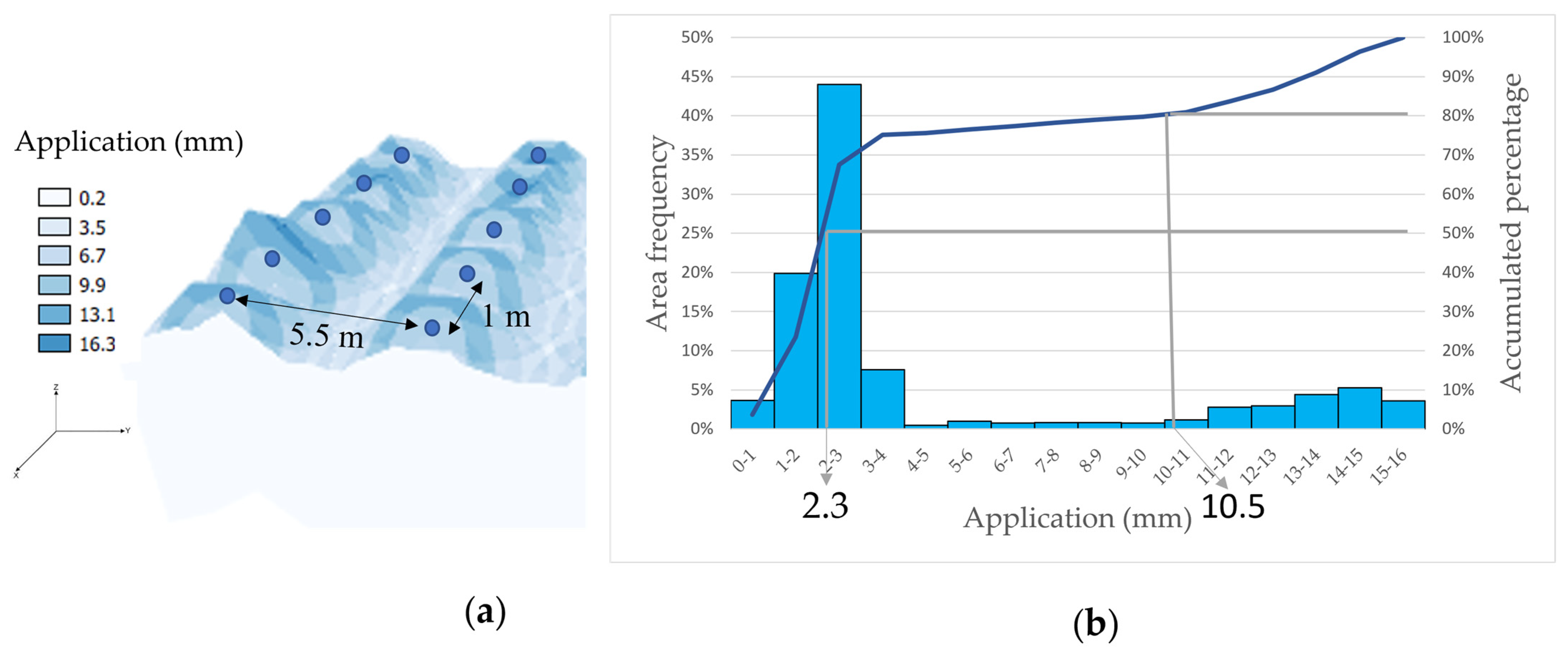
The simulation yielded the geospatial representation of water application by sprinklers in all sectors (see one example in Figure 4a). In total, two raster representations were obtained, that is, the situation with the maximum pressure and the situation with the minimum pressure. The representation, which can be viewed in QGIS, was converted into a flat data file, and manipulated with the Excel program to obtain, among other things, the histogram of rainfall frequencies for each sector, as shown in Figure 4b.
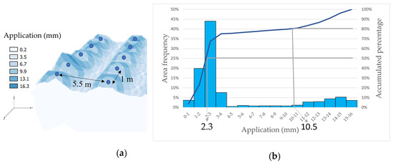
Figure 4.
(a) Geospatial representation of rainfall in an area of sector 1 with an irrigation duration of 30 min (b) Frequency histogram of sector 1 (light blue bars) and accumulated percentage (dark blue line).
The histogram shown in Figure 4b shows the distribution of the water height values of each pixel, in percent area. The histogram shown is the one obtained after the simulation of sector 1. Each range of the x-axis agglutinated all the pixels that had a value between these values and were projected onto the y-axis where the percentage of the area is shown. In this case, range 2–3 had a value of 44%, which meant that 44% of the area received between 2 and 3 mm of water. The histogram showed the application’s average height over the entire surface (2.3 mm), which was approximately equal to the median. Half of the surface was irrigated with 2.3 mm or more, while the other half was irrigated with 2.3 mm or less. This value could be compared with the theoretical average design head of 10.5 mm obtained from the flow rate provided by the sprinklers in the sector (2 L/min), the number of sprinklers, and the area they cover. Figure 4 shows that at least this height of water irrigated only 20% of the area.
Starting from the spatially located rainfall data, the distribution uniformity for the desired areas could be calculated from the same data file. In the case of calculating distribution uniformity within the sector, it can be calculated at various scales. One of them is to take the data from a 10 m2 moving window, which would give the distribution uniformity coefficient values shown in Figure 5.
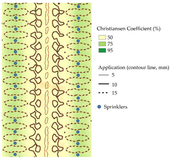
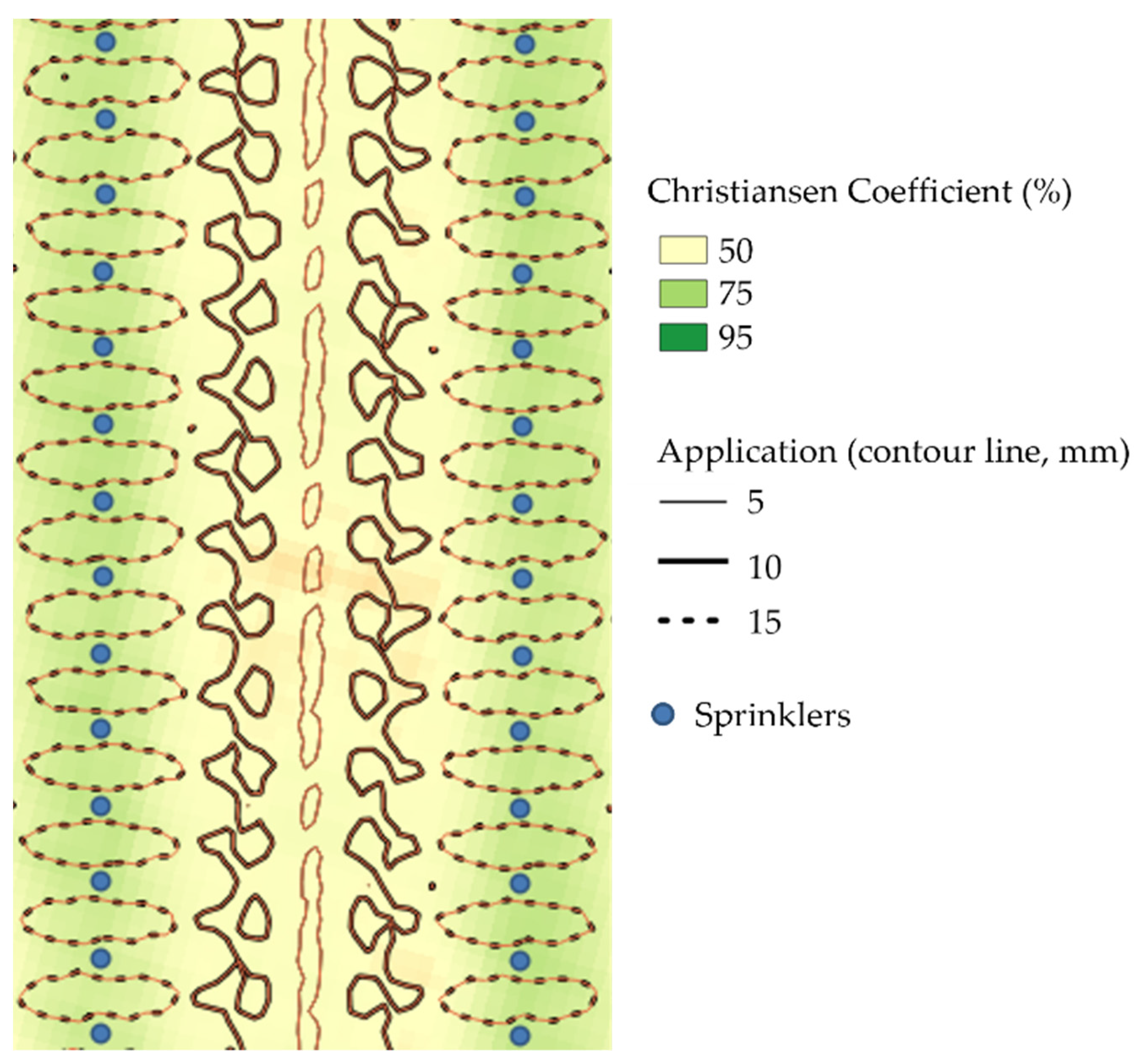
Figure 5.
Christiansen’s uniformity coefficient calculated on an area of 10 m2 in a sector with the rainfall contour lines at a distance of 5 mm.
Figure 5 shows the distribution uniformity that each pixel had if the data were taken 10 m2 around it. Greener values imply greener uniformities than yellower ones. As can be seen, the distribution uniformity was higher in the area closer to the emitters, because the amount of water that ended up falling was more similar than in the center of the tunnel. In the center of the tunnel, as there were areas with low rainfall and areas with higher rainfall (those closest to the emitters) the uniformity was lower.
Following the methodology already explained and shown in the previous example, the distribution uniformity could also be calculated for the whole sector. To further illustrate the possibilities of the tools developed in this work, the uniformity coefficient for each sector was calculated for the maximum and minimum pressure conditions, previously identified following the procedure explained in Section 2.4 (Figure 6).

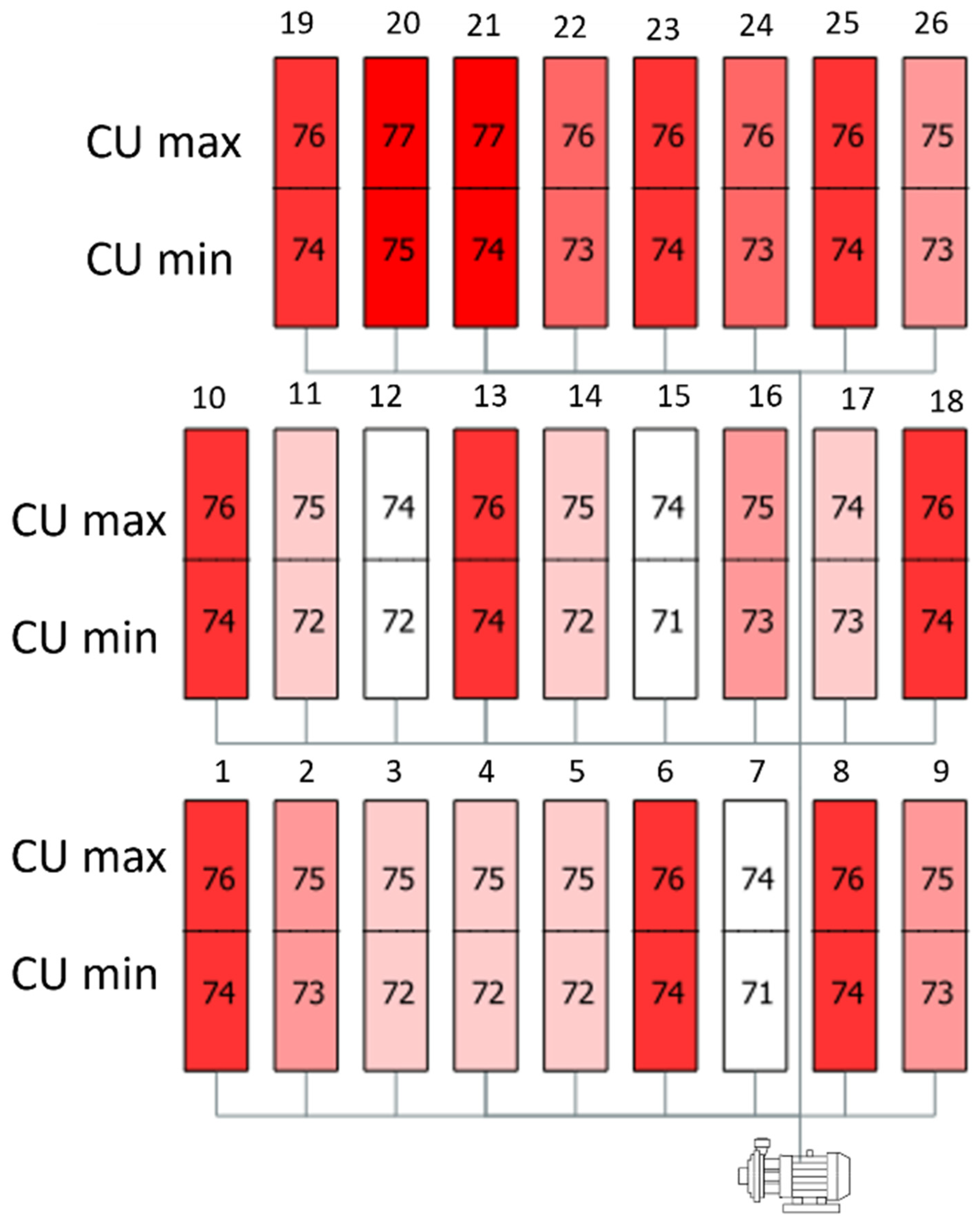
Figure 6.
Christiansen’s uniformity coefficient for each sector at maximum pressure (upper value) and minimum pressure (lower value).
These values show the uniformity in each sector depending on the sectors opened. The maximum uniformity was the uniformity of the sector when it was open with the two sectors that make the uniformity maximum, while the minimum uniformity was the uniformity in the opposite situation. For example, in the case of sector 1, the value of 76% shows that when sector 1 was open with the combination of sectors that mad the pressure maximum in sector 1, the distribution uniformity would be 76%. In the opposite case, when the combination of tunnels made the pressure minimum in sector 1, the distribution uniformity would be 74%. The variation between the uniformity data of the different sectors was due to the fact that the number of emitters in each sector, and therefore the demand, was different. Furthermore, in this simulation, given the proportionality between the arrival pressure and the distribution uniformity, it will be possible to achieve greater uniformity in the farm, optimizing its management, which can be of great importance in sensitive or high value-added crops.
These data, in turn, were compared with those obtained in the distribution uniformity study. For each sector in which the uniformity study was carried out, the data of the Christiansen’s uniformity coefficient measured in the studied area (Equation (1)) and the one obtained by extrapolation to the sector in which it was located (Equation (2)) are shown. In addition, the data obtained from the simulation are shown for the whole sector when the pressure was at its maximum and minimum (Table 3).
Table 3.
Comparison of measured and simulated Christiansen’s uniformity coefficients.
As can be seen, the simulated and measured CU were very similar. The most significant difference was an underestimation of 5.76%. Considering that the simulations considered the most extreme situations, it was expected that the value of the field evaluation would be between the two. Although this was not the case, the measured and simulated data were very similar.
4. Discussion
This work aimed to simulate the precipitation applied by sprinklers in greenhouse facilities and to know in detail the uniformity of this precipitation. For this, the integration of two computer tools such as QGIS and EPANET, was proposed. The simulation developed in this study obtained results similar to those in reality. Furthermore, it has been shown that the distribution uniformity of a sector calculated by using rain gauges in one area and extrapolating them to the whole sector can be simulated by means of the tools and methodology proposed.
Unlike previous studies, this simulation effort made it possible to adapt to the peculiarities of a given irrigation installation. Compared to other established models, the integration between EPANET and QGIS was much more flexible. Among other things, it has made it possible to obtain distribution uniformity at various scales. It has also made it possible to rank the combination of sector openings based on distribution uniformity. In addition, using a hydraulic simulation program such as EPANET, other important variables for hydraulic evaluations such as pump efficiency have been calculated, and the combination of sector openings can again be ordered according to pump efficiency. This work therefore opens the way for new projects that aim to determine the behavior of the irrigation system from hydraulic simulations.
The methodology proposed in this article is susceptible to incorporating a series of improvements related to the evaluation of the sprinklers and the evaluation of the simulations with an in situ experimentation. This could be performed mainly by increasing the number of laboratory sprinkler evaluations and using several sprinklers. In addition, a larger number of sectors could be compared between simulated and measured data, which would help to improve the model more accurately. However, the idea of simulating the hydraulic behavior of a complete greenhouse sprinkler irrigation system by integrating GIS and hydraulic simulation tools using open-source software could become a very valuable tool for evaluating irrigation systems. In addition, this avoids the rigidity of the input data of previous studies where there was hardly any possibility of adding the particularities of a specific installation. Estimating the distribution uniformity over the entire surface without the need to measure it directly saves a lot of effort and resources and allows on many occasions to know data that otherwise would be very difficult to obtain. In short, we believe that the methodology proposed in this article can be very useful to improve the management of sprinkler irrigation systems, particularly those in which distribution uniformity is of special importance, as is the case of high value-added crops, which are frequently grown in greenhouses. It has been shown that it is possible to accurately estimate distribution uniformity in different areas of a facility. This will allow actions such as: (i) assigning the areas with greater uniformity to the most demanding or cost-effective crops; (ii) identifying areas where an improvement of the facilities would be desirable; (iii) identifying the tunnel opening combinations that improve uniformity in each of them. These improvements in management could also result in savings in water and other inputs, which are becoming increasingly important in the current context of climate change and the reduction in the impact of agriculture on the environment. Finally, similar studies could be carried out with the same tools for other pressurized irrigation systems, such as sprinkler irrigation outside greenhouses and drip irrigation.
5. Conclusions
Given the similarity between the measured and simulated results (biggest difference of 5.76% among sectors), the integration of GIS tools with hydraulic simulation tools has been proven to have good results when estimating the distribution uniformity.
As with any other simulation model, it is not a completely real image of the reality, but it helps a lot to make a realistic estimation taking into account the particularities of an irrigation installation. This model, therefore, will serve as a tool that will allow the distribution uniformity in the irrigation installation to be known in a general way, but the results obtained will not be completely accurate. The model created has a lot of room for improvement and needs to be calibrated and validated with further evaluations. It is expected that, in the not-too-distant future, such flexible tools will become part of irrigation evaluations.
Supplementary Materials
The following supporting information can be downloaded at: https://www.mdpi.com/article/10.3390/su14159723/s1.
Author Contributions
I.B.: Conceptualization, Data curation, Formal analysis, Investigation, Methodology, Resources, Software, Validation, Visualization, Writing—original draft, Writing—review and editing. M.Á.C.-B.: Conceptualization, Project administration, Resources, Supervision, Writing—review and editing. J.C.: Conceptualization, Project administration, Resources, Supervision, Writing—review and editing. All authors have read and agreed to the published version of the manuscript.
Funding
Research Initiation Grant of the Public University of Navarra for master’s students who develop their Master’s Thesis (TFM) in the field of research institutes and in Navarrabiomed, academic year 2021–2022 (Res 602/2022).
Institutional Review Board Statement
Not applicable.
Informed Consent Statement
Not applicable.
Data Availability Statement
Not applicable.
Conflicts of Interest
The authors declare no conflict of interest.
References
- The World Bank. Water in Agriculture. 2020. Available online: https://www.worldbank.org/en/topic/water-in-agriculture#1 (accessed on 28 November 2021).
- Ministerio de Agricultura P y A. Encuesta sobre Superficies y Rendimientos de Cultivos Publicación elaborada por la Ministerio de Agricultura, Pesca y Alimentación. 2021. Available online: https://cpage.mpr.gob.es (accessed on 20 April 2022).
- Ministerio de Agricultura P y A. Encuesta Sobre Superficies y Rendimientos. 2020. Available online: https://cpage.mpr.gob.es (accessed on 20 April 2022).
- FAO. Water. 2021. Available online: https://www.fao.org/water/en/ (accessed on 9 April 2021).
- Eng, M.J.A.; Sehsah, E.M.E.; El Baily, M.M.; Aiad, M.; Prof, A. Irrigation and Drainage Evaluation of a Single Sprinkler under Egyptian Microclimate Conditions. 2014. Available online: https://journals.ekb.eg/article_98903_59958490934e90d7b0920030c8f498d6.pdf (accessed on 26 April 2022).
- Playán, E.; Zapata, N.; Faci, J.M.; Tolosa, D.; Lacueva, J.L.; Pelegrín, J.; Salvador, R.; Sánchez, I.; Lafita, A. Assessing sprinkler irrigation uniformity using a ballistic simulation model. Agric. Water Manag. 2006, 84, 89–100. Available online: https://reader.elsevier.com/reader/sd/pii/S0378377406000266?token=F74D1089E709B1600B09FFCB7374D506FC02D301D25620373E494C314B62A5C34D22BB7D78FFF1F4332662F1DE24B39D&originRegion=eu-west-1&originCreation=20211109081108 (accessed on 11 April 2022). [CrossRef] [Green Version]
- Li, Y.; Bai, G.; Yan, H. Development and validation of a modified model to simulate the sprinkler water distribution. Comput. Electron. Agric. 2015, 111, 38–47. [Google Scholar] [CrossRef]
- Zhang, L.; Merkley, G.P.; Pinthong, K. Assessing Whole-Field Sprinkler Irrigation Application Uniformity. 2011. Available online: https://link.springer.com/content/pdf/10.1007/s00271-011-0294-0.pdf (accessed on 9 November 2021).
- Chen, Z.; Duan, F.; Fan, Y.; Jia, Y.; Huang, X. Static simulation on water distribution characteristics of overlap area and whole spraying area for sprinkler. Nongye Gongcheng Xuebao/Trans. Chin. Soc. Agric. Eng. 2017, 33, 104–111. [Google Scholar]
- Do Prado, G.; Colombo, A. Spatial distribution of water applied by traveler irrigation machines—Part II: Simulasoft validation. IRRIGA 2010, 15, 63–74. [Google Scholar]
- Fukui, Y.; Nakanishi, K.; Okamura, S. Computer evaluation of sprinkler irrigation uniformity. IRRIG Sci. 1980, 2, 23–32. [Google Scholar] [CrossRef]
- CIT. Space Pro. 2022. Available online: https://www.fresnostate.edu/jcast/cit/software/ (accessed on 20 April 2022).
- Tarjuelo, J.M.; Carrión, P.; Montero, J. SIRIAS: A Simulation Model for Sprinkler Irrigation. 2001. Available online: https://link.springer.com/content/pdf/10.1007/s002710000031.pdf (accessed on 11 April 2022).
- Pérez-Padillo, J.; Morillo, J.G.; Poyato, E.C.; Montesinos, P. Open-source application for water supply system management: Implementation in a water transmission system in southern spain. Water 2021, 13, 3652. [Google Scholar] [CrossRef]
- Muller, L.; Gericke, J.; Pietersen, J. Methodological approach for the compilation of a water distribution network model using QGIS and EPANET. J. S. Afr. Inst. Civ. Eng. 2020, 62, 32–43. [Google Scholar] [CrossRef]
- Safitri, A.; Wahyudi, S.I. Simulation of Transmission of Drinking Water Sources to Reservoirs: Case Study PDAM Tirta Jati, Cirebon, Indonesia. In Proceedings of the 5th International Conference on Civil and Environmental Engineering for Sustainability, Johor, Malaysia, 19–20 December 2019; IOP Publishing: Bristol, UK, 2020; Volume 498. [Google Scholar]
- Estong, I.; Perez, C.; Ansagay, N.; Carbon, M.; Ugalde, J.; Lubrica, N.; Tandy, P.; Apnoyan, H.; Anama, W. Sustainable rainwater harvesting system. J. Adv. Res. Dyn. Control. Syst. 2020, 12, 1107–1122. [Google Scholar]
- Nagarajan, K.; Charhate, S. Application of geographic information system for water distritbution networks through quantum gis plug-in with hydraulic simulation for infrastructure and development planning. In Proceedings of the 38th Asian Conference on Remote Sensing—Space Applications: Touching Human Lives, ACRS 2017, New Delhi, India, 23–27 October 2017. [Google Scholar]
- Gholami, V.; Asghari, A.; Taghvaye Salimi, E. Flood hazard zoning using geographic information system (GIS) and HEC-RAS model (Case study: Rasht City). CJES 2016, 14, 263–272. [Google Scholar]
- Alemi Safaval, P.; Kheirkhah Zarkesh, M.; Neshaei, S.A.; Ejlali, F. Morphological changes in the southern coasts of the Caspian Sea using remote sensing and GIS Morphological changes in the southern coasts of the Caspian Sea using remote sensing and GIS. Casp. J. Environ. Sci. 2018, 16, 271–285. [Google Scholar]
- Pérez Urrestarazu, L.; Díaz, J.A.R.; Poyato, E.C.; Luque, R.L.; Jaraba, F.M.B. Development of an integrated computational tool to improve performance of irrigation districts. J. Hydroinform. 2012, 14, 716–730. [Google Scholar] [CrossRef] [Green Version]
- Christiansen, J.E. Agricultural Experiment Station Irrigation by Sprinkling. 1942. Available online: https://brittlebooks.library.illinois.edu/brittlebooks_closed/Books2009-04/chrije0001irrspr/chrije0001irrspr.pdf (accessed on 11 April 2022).
- Keller, J.; Bliesner, R.D. Sprinkler and Trickle Irrigation; Van Nostra: New York, NY, USA, 1990; 652p. [Google Scholar]
- QGIS. Bienvenido al Proyecto QGIS! 2022. Available online: https://qgis.org/es/site/index.html (accessed on 29 April 2022).
- United States Environmental Protection Agency. EPANET | US EPA. 2022. Available online: https://www.epa.gov/water-research/epanet (accessed on 21 April 2022).
- Eusuff, M.M.; Lansey, K.E. Optimization of Water Distribution Network Design Using the Shuffled Frog Leaping Algorithm. J. Water Resour. Plan. Manag. 2003, 129, 1–8. [Google Scholar] [CrossRef]
- Díaz, J.A.R.; Luque, R.L.; Cobo, M.T.C.; Montesinos, P.; Poyato, E.C. Exploring energy saving scenarios for on-demand pressurised irrigation networks. Biosyst. Eng. 2009, 104, 552–561. [Google Scholar] [CrossRef]

Publisher’s Note: MDPI stays neutral with regard to jurisdictional claims in published maps and institutional affiliations. |
© 2022 by the authors. Licensee MDPI, Basel, Switzerland. This article is an open access article distributed under the terms and conditions of the Creative Commons Attribution (CC BY) license (https://creativecommons.org/licenses/by/4.0/).