A New Measurement of Global Equity in a Sustainability Perspective: Examining Differences from Space and Time Dimensions

Abstract

With the increasing development gap, how to measure global equity in the perspective of sustainability has become an essential issue nowadays. To examine the intra-generational equity from the space dimension and the inter-generational equity from the time dimension, a new measurement of global equity in a sustainability is proposed in this paper. Firstly, a comprehensive assessment index of regional development and an index of regional equity are constructed based on panel data using an entropy weight method (EVW) and a coefficient of variation method (CVM). Secondly, the intra-generational equity within different continents and echelons and the inter-generational equity in seven fields over the last 30 years are analyzed. Lastly, the global equity index for the next 10 years is predicted based on a panel data autoregressive model. The results of the study will be a reference for global equity strategies.

1. Introduction

The global sustainable development strategy—“Agenda 21” [1] was proposed and passed at the United Nations Conference on Environment and Development held in Rio de Janeiro, Brazil in June 1992. Since then, most countries have formulated sustainable development strategies, plans, and countermeasures according to their own conditions. Among the three basic principles of sustainable development, the principle of equity is the one that concerns people most [2,3]. Specifically, the principle of equity considers sustainable development as a development with equal opportunities and benefits [4]. It includes both intra-generational equity, which means that the development of one region should not be at the expense of the development of other regions [5], and inter-generational equity, which means that the needs of the present generation are met without compromising the development capacity of future generations [6].

Due to the abstractness of the concept of equity, many scholars studied equity subjectively from a qualitative perspective [7,8,9,10]. Some literature studied equity from a quantitative perspective by using mathematical methods [11,12,13]. However, these researches only considered a particular field, ignoring the overall impacts of equity changes. Moreover, some scholars tend to focus on a single dimension of inter-generational equity or intra-generational equity, ignoring the potential conflicts of equity principles of different dimensions [14,15,16,17,18].

To overcome the above limitations, we try to construct a regional equity evaluation index combining qualitative and quantitative methods. It will cover multiple fields and be used to analyse both intra-generational and inter-generational equity. This is the main objective of our paper.

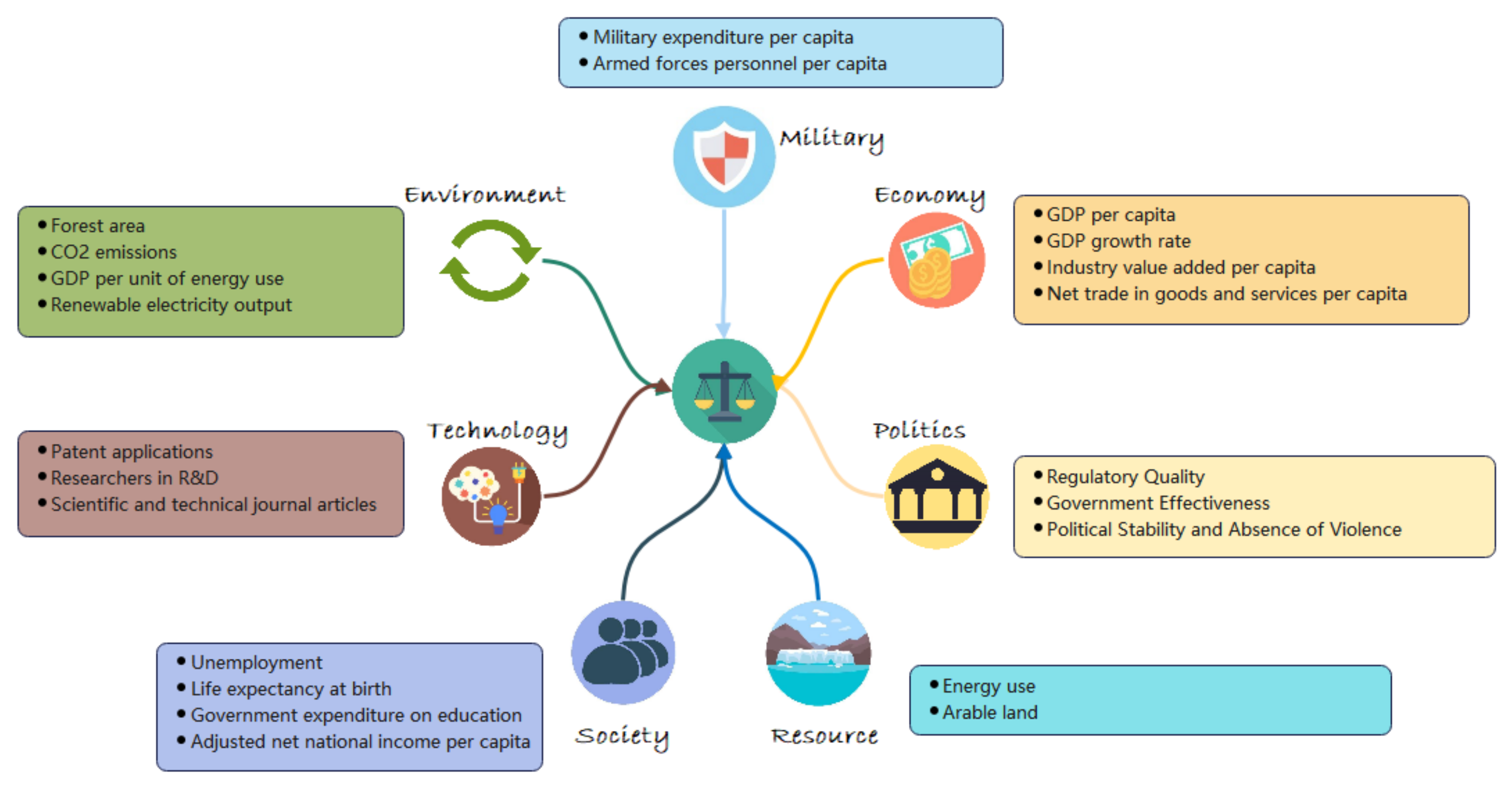
To give the definition of regional equity, we need to define the level of development of a country. Referring to the classical index systems such as the national development level evaluation systems proposed by Hu Angang et al. [19] and B.N. Kuzyk et al. [20], we select a total of 22 indicators in seven fields to build a comprehensive evaluation system, including economy, military, politics, resources, society, sustainability, and technology. Then, we define a regional equity index by the variability of the development level of the countries in this region. The coefficient of the variation method and the entropy weight method based on panel data including different countries and years will be used in constructing the indicators system. It not only allows us to compare differences in equity across continents from the space dimension, i.e., intra-generational equity, but also analyze and predict changes in global or regional equity from the time dimension, i.e., inter-generational equity.

The rest of the article is organized as follows. A brief literature review on equity and development is provided in Section 2. In Section 3, a comprehensive assessment index of equity is constructed based on panel data. In Section 4, the index is applied to analyze global equity from space and time dimensions, respectively. Conclusions and future research directions are presented in Section 5.

2. Literature Review

The trend of sustainable development has driven people to consider the significance of equity in development. Over the past two decades, there has been much literature discussing the connections between equity and sustainable development. See Templet [21], Daily and Ehrlich [22], Spijkers et al. [23] and Martinet et al. [24] as well.

As described in the introduction, equity under sustainability includes both intra-generational equity and inter-generational equity. However, in recent decades, scholars have paid more attention to the concept of equity in terms of opportunity equity (i.e., equity of expected benefits ex ante) and outcome equity (i.e., equity of benefits ex post) [25]. Kodelja et al. [26] find that equal educational opportunities ultimately lead to unequal educational outcomes due to individual differences among students. Magni et al. [27] and Phillips et al. [28] argue that opportunity equity may only be a condition leading to outcome equity. Considering the inherent differences between countries and the availability of data, we decided to measure equity from the outcome equity aspect, defining equity as the situation of differences in the development level within a region.

With the increasing gap in overall social development, more and more scholars are interested in how to measure the global or regional equity from different perspectives. The economy is an important aspect that concerns many scholars. Pearce [29] discussed the relationship of economics, equity, and sustainable development. Later, Padilla [6] pointed out the limitations of traditional economic analysis based on inter-generational equity. Recently, Stokan et al. [30] suggested that governments are more likely to adopt economic development policies to promote equity when they have less competitive pressures, greater resource capacity, and more opportunities to participate in economic development planning. There exist some researchers who study equity from an environmental perspective. Okrent et al. [14] examined the intertwined matters of inter-generational equity and the discounting of future health effects while discussing the conflict between intra-generational equity and inter-generational equity. Xu et al. [31] integrated intra- and inter-generational equity using a Gini coefficient and a modified Bentham–Rawls criterion to allow for time and space social equity trade-offs for sustainable water allocation. Araos et al. [32] assessed how social equity was integrated into climate change adaptation and suggested actions for the equity of adaptation by systematically analyzing the participation of marginalized groups in environmental policies. More literature considers this issue from a social perspective. Hackl et al. [33] proposed a mobility equity framework for all forms of social, human, and digital mobility and provided new ideas for considering research and policy making within the broader inequality–mobility nexus of global development. Braveman et al. [34] provided a carefully constructed definition of health equity and discussed the definition’s implications both for action and for assessing progress toward health equity. Akmal et al. [35] studied the inequality in learning goals and achievements between the rich and poor in five developing countries and noted that it was necessary to make progress in education for all to achieve global equity.

Note that the above research studies are all qualitative. More and more scholars have conducted quantitative analyses of equity in various fields with mathematical models. Czarny et al. [36] analyzed economic efficiency and equity with quantitative indicators and showed that Sweden and other Nordic countries have not only achieved some of the best economic outcomes in the world, but also successfully reduced the scale of social inequality and ensured relatively equal citizen opportunities. Steffen et al. [37] combined equity considerations with a biophysical planetary boundary approach to investigate the relationship between equity and environmental sustainability. Chapman et al. [38] investigated five critical social equity impacts of environmental improvement, health, employment, participation, and energy cost from a viewpoint of an equitable energy transition, using indicators relevant to energy policy and the energy transition. Omoeva et al. [39] used an output-driven approach to measure the equity of educational resource allocation by dividing educational resources into three dimensions: teacher quality, school physical environment, and school instructional environment. Jason et al. [40] measured country responsibility for ecological damage and equity in allocating ecological resources by assessing the country’s cumulative use outside of equitable and sustainable boundaries.

However, the above studies mainly focus on quantitatively analyzing equity in a particular field and cannot provide a comprehensive picture of global or regional equity. As far as we know, there is little literature that takes a macro perspective and comprehensively considers regional equity in multiple fields. Therefore, we construct a comprehensive evaluation system of regional development level with multiple field indicators and calculate the regional equity index to fill this gap. The development level evaluation systems serve as an important tool for measuring development results. They have widely concerned scholars since the concept of developed countries was introduced in the 1950s, and some are still available nowadays. The early Global Competitiveness Index (GCI) describes the development environment for firms’ international competitiveness within a region by synthesizing the balance between the fundamental forces of firms. Competitiveness evaluation is related to development evaluation, but there are certain differences in the evaluation subject, evaluation focus, and evaluation methods. Moreover, the Human Development Index (HDI) has been launched by the United Nations Development Programme (UNDP) and much mentioned in recent years. It can reflect differences in human development levels of different countries by measuring the average achievement in three basic dimensions: life expectancy, knowledge, and standard of decent living. The HDI can evaluate the final development achievement, but it cannot reflect the change of factors and lacks dynamicity [41]. To the best of our knowledge, there is no mainstream evaluation system of development level nowadays.

In the last two decades, some scholars have proposed new ideas on this topic. Cheng et al. [42] used principal components to assess the comprehensive national power of 11 important countries in 2010. Song et al. [43] quantitatively assessed the comprehensive national power of 19 sovereign countries in 2016 from eight dimensions, economy, society, and sustainable development, etc. However, all of the above assessment methods are based on cross-sectional data and cannot compare and predict country development level from the time dimension. To overcome this, we use panel data to establish a comprehensive evaluation system of regional development level and calculate a regional equity index. It not only allows us to analyze intra-generational equity from the space dimension, but also inter-generational equity from the time dimension.

Because our methods are based on panel data, it allows for a comprehensive analysis of both intra-generational and inter-generational equity in both space and time dimensions, rather than just intra- or inter-generational equity as in previous studies.

In summary, compared with the existing literature, the contributions of our paper are mainly as follows. (1) Combining qualitative and quantitative methods, a new measurement of region equity covering multiple fields is proposed in our paper. It will overcome the shortcomings of previous studies that typically evaluate equity only qualitatively or only quantitatively examine the equity in a particular field. (2) Because our methods are based on panel data, they allow for a comprehensive analysis of both intra-generational and inter-generational equity from space and time dimensions, rather than just intra- or inter-generational equity as in previous studies.

3. Materials and Methods: Assessment Index of Global Equity

To assess global equity, we initially construct the Region Development Index (RDI) to measure the development level of a region. Then we define the Regional Equity Index (REI) based on the RDI.

3.1. Selection of Evaluation Indicators

As pointed out in “Agenda 21”, sustainable development includes economic, social, and ecological sustainability. To scientifically and comprehensively evaluate the development level of a country, we refer to the studies of Hu et al. [19] and Kuzyk et al. In [20], the authors establish an evaluation system with seven first-level indicators including economy, military, politics, resources, society, environment, and technology. Each first-level indicator includes 2 to 4 secondary indicators, with a total of 22 indicators. The constructed development level evaluation indicator system is shown in Figure 1. And the specific description of each indicator is as follows.

(1)

Economy

The economic foundation determines the superstructure. Without a prosperous economy and healthy trade activities, other aspects of development will encounter obstacles and the overall level of development will be difficult to improve. GDP per capita and GDP growth rate are important indicators to evaluate the level of economic development. Industry is the strong support for the regional economy, and we use industry value added per capita to measure the development level of regional industry. Since services occupy an important place in the composition of the current economy and healthy trade symbolizes the economic dynamism of the region, we chose net trade in goods and services per capita.

(2)

Military

A strong military power is a guarantee of stable regional development. Military factors are reflected through two indicators: military expenditure per capita, which is concerned with the quality of force construction and development; armed forces personnel per capita, which determines the amount of combat power at disposal.

(3)

Politics

The development of a region is inseparable from the leadership of the government. A capable government can properly lead regional development. The political factor contains three indicators: political stability, a stable political situation is a guarantee for development, and a turbulent regime is often detrimental to development; government effectiveness, an efficient and high-quality government is a strong driver of development; and regulatory quality, effective regulation can promote the implementation of the policy.

(4)

Resources

Abundant resources are an important guarantee for regional development. If a region has abundant resources, its development will be full of power and energy. Hence, we choose energy use per capita and arable land per capita to evaluate the resources of a region.

(5)

Society

The social situation is an important factor in assessing the development level of a region. Society includes education, quality of life, and other aspects. We choose the following four indicators to assess it. Since the health of the population and the investment in education are important reflections of the level of human resources, life expectancy at birth and total government expenditure on education as a percentage of GDP are chosen. Disposable income of residents symbolizes the development level of the society, and accordingly adjusted net national income per capita is chosen as an indicator. Stable employment is crucial to social stability, and total unemployment rate is chosen as a measure in this paper.

(6)

Environment

The Rio Declaration stated that “for sustainable development, environmental protection must be an essential part of the development process, and the process cannot be considered in isolation from it.” [44]. Clean energy and the efficient use of energy are important components of sustainable development. Then, we choose the following four indicators: GDP per unit of energy use, renewable electricity output as a percentage of total generation, CO₂ emissions, and forest area as a percentage of land area as metrics of environment.

(7)

Technology

Advanced technology can greatly accelerate the development of a region, so it is one of the important factors to measure development level. We measure technology factors by three indicators: researchers in R&D, the size of the scientific team can reflect the existing technological strength; patent applications, the application of scientific patents represents the technological innovation capacity; and scientific and technical journal articles, which represent the fruitfulness of the technological achievements and symbolize the impact of science.

3.2. Calculation of the Weights

In this section, we propose a method to calculate the weights based on panel data. Firstly, we apply the entropy weight method (EWM) to calculate the weights of second-level indicators. Then we use the coefficient of variation method (CVM) to calculate the weights of first-level indicators.

3.2.1. Weights of Second-Level Indicators

The basic idea of the EWM is to assign weights according to entropy values of indicators. The smaller the entropy value of an indicator is, the more information it provides, and the greater weight it has and vice versa. A detailed theory of the EWM can be found in the literature [45].

For narrative convenience, let $x_{ijt}^a$ be the value of the jth second-level indicator corresponding to the ith first-level indicator in year t of country a, $i=1,\cdots ,k;j=1,\cdots ,m_i;t=1,\cdots ,T;a=1,\cdots ,N$. The steps for calculating the weights of the second-level indicators are given in the following.

Step 1: Indicator standardization

Positive indicator: the larger the better, such as GDP per capita, R&D expenditure, etc.

$$z_{ijt}^a=\frac{x_{ijt}^a-x_{ij,min}}{x_{ij,max}-x_{ij,min}}$$

(1)

Negative indicator: the smaller the better, such as greenhouse gas emissions, etc.

$$z_{ijt}^a=\frac{x_{ij,max}-x_{ijt}^a}{x_{ij,max}-x_{ij,min}}$$

(2)

where, $x_{ij,max}=\underset{t,a}{max}\left\{x_{ijt}^a\right\},x_{ij,min}=\underset{t,a}{min}\left\{x_{ijt}^a\right\}$

Step 2: Indicator normalization

$$p_{ijt}^a=\frac{z_{ijt}^a}{{\sum }_{t=1}^T{\sum }_{a=1}^N{z}_{ijt}^a}$$

(3)

Step 3: Calculate the entropy value

$$e_{ij}=-\frac{1}{ln\left(NT\right)}\sum _{t=1}^T\sum _{a=1}^N{p}_{ijt}^{a}ln\left(p_{ijt}^a\right)$$

(4)

Step 4: Calculate second-level indicator weight

$$w_{ij}=\frac{1-e_{ij}}{{\sum }_{j=1}^{m_i}(1-e_{ij})}$$

(5)

3.2.2. Weights of First-Level Indicators

The basic idea of the coefficient of variation method is that in the evaluation indicators system, the greater the variance of the indicator, the more it can distinguish the evaluation object. Therefore, the indicator should receive greater weight and vice versa.

By the weights of the second-level indicators, the score of the i-th first-level indicator in year t of country a can be calculated:

$$u_{it}^a=\sum _{j=1}^{m_i}{w}_{ij}·p_{ijt}^a$$

(6)

Step 1: Calculate the mean and standard deviation of the ith first-level indicator

$${\overline{u}}_i=\frac{1}{NT}\sum _{a=1}^N\sum _{t=1}^T{u}_{it}^a,s_i{}^2=\frac{1}{NT-1}\sum _{a=1}^N\sum _{t=1}^T{(u_{it}^a-{\overline{u}}_i)}^2$$

(7)

Step 2: Calculate the coefficient of variation of the ith first-level indicator

$$v_i=\frac{s_i}{{\overline{u}}_i}$$

(8)

Step 3: Calculate the weight of the ith first-level indicator

$$w_i=\frac{v_i}{{\sum }_{i=1}^k{v}_i}$$

(9)

3.3. Regional Development Index and Regional Equity Index

Now, we can construct the RDI for country a in year t, denoted by $RD{I}_t^a$, as follows.

$$RD{I}_t^a=\sum _{i=1}^k{w}_i{u}_{it}^a=\sum _{i=1}^k\sum _{j=1}^{m_i}{w}_i{w}_{ij}{p}_{ijt}^a,t=1,\cdots ,T;a=1,\cdots ,N$$

(10)

Clearly, the higher the RDI a region has, the better overall development level it possesses.

It is important to note that global equity does not mean that every country can obtain the same resources and opportunities, but rather that through prioritized resource allocation, countries can achieve relative balance on multiple dimensions of development. Hence, we use the variation of the RDI to measure regional equity. The greater the variation of the RDI is, the worse the equityis. Therefore we define the standard deviation of the RDI as the REI.

$$REI=std\left(RDI\right)$$

(11)

4. Application

4.1. Weights Results

To provide a comprehensive representation of the global situation, we select 45 countries covering different levels of development from six continents, excluding Antarctica, as a sample according to the current UN classification of developed, developing, and least developed countries. Focusing on the global scale, the countries we have selected at different levels of development are not evenly distributed, with more developed countries concentrated in Europe, the major component of Asia being developing countries, and the least developed countries concentrated in Africa. The selected countries in each continent are shown in

Table 1. Distribution of countries by continents.

Asia	Africa	Europe	South America	North America	Oceania
China	Algeria	Denmark	Argentina	Canada	Australia
India	Egypt, ArabRep.	Finland	Bolivia	United States	New Zealand
Japan	Ethiopia	France	Brazil	Mexico
Malaysia	Kenya	Germany	Chile
Mongolia	Morocco	Italy	Colombia
Pakistan	Tanzania	Netherlands	Peru
Philippines	Tunisia	Norway	Venezuela, RB
Saudi Arabia	Zambia	Poland
Thailand		Portugal
Turkey		Russian Federation
		Spain
		Sweden
		Switzerland
		United Kingdom
		Ukraine

.

We obtain the corresponding panel data from 1990 to 2019 for 45 selected countries from the World Bank and Worldwide Governance Indicators (WGI). With the proposed method above, the weights of indicators at each level are shown in

Table 2. The weights of each indicator in the RDI model.

Comprehensive Index	First-Level Indicator	Weight1	Second-Level Indicator	Weight2
RDI	Economy	0.2428	GDP per capita (current US$) (E1)	0.4747
			Industry(including construction), value added per capita (current US$) (E2)	0.4404
			Net trade in goods and services per capita (current US$) (E3)	0.0763
			GDP growth rate (current dollars) (E4)	0.0087
	Military	0.1949	Military expenditure per capita (current US$) (M1)	0.7654
			Armed forces personnel per capital (M2)	0.2346
	Politics	0.0774	Political Stability and Absence of Violence/Terrorism (P1)	0.5186
			Government Effectiveness (P2)	0.2519
			Regulatory Quality (P3)	0.2295
	Resources	0.0539	Energy use (kg of oil equivalent per capita) (R1)	0.4854
			Arable land (hectares per person) (R2)	0.5146
	Society	0.2059	Adjusted net national income per capita (current US$) (C1)	0.8431
			Life expectancy at birth, total (years) (C2)	0.0613
			Unemployment, total (% of total labor force) (modeled ILO estimate) (C3)	0.0275
			Government expenditure on education, total (% of GDP) (C4)	0.0680
	Sustainability	0.0612	GDP per unit of energy use (PPP $ per kg of oil equivalent) (S1)	0.0468
			Renewable electricity output (% of total electricity output) (S2)	0.5432
			CO2 emissions (metric tons per capita) (S3)	0.0818
			Forest area (% of land area) (S4)	0.3281
	Technology	0.1638	Researchers in R&D (per million people) (T1)	0.2360
			Patent applications (T2)	0.4926
			Scientific and technical journal articles (T3)	0.2714

.

4.2. Analysis from Space Dimension

4.2.1. Geographical Location

To study the equity status of development levels within different regions worldwide, we calculate the RDI of countries within each continent and take the average as the continental RDI to reflect the development level of the continent. The results of the RDI and REI for the six continents in 2019 are shown in

Table 3. RDI and REI of six continents.

Continent	Asia	Africa	Europe	South America	North America	Oceania
RDI	6.4557	2.3732	14.0420	4.4609	15.0212	15.4363
REI	5.498	0.5437	5.6218	0.9877	9.1039	3.0627

.

We find that Africa and South America have the best within-continent equity with REI less than 1, but these two continents have correspondingly the lowest RDI, both less than 5. The possible reason why these two continents can achieve a higher equity level is that their development level is lower. Asia, Europe, and Oceania have worse equity compared to the former. It is worth noting that Oceania and Europe not only have good results in equity, but also have excellent performance in region development level, with the RDI in first and third place, respectively, and much more than the fourth place continent. the RDI in North America is in second place but has the worst intra-continental equity, far greater than the remaining five continents, which reflects the extreme imbalance in the development of countries in North America.

4.2.2. Development Level

To explore the regional equity status among countries with different development levels, we divide the selected countries into three echelons according to the development level of each field in 2019 by K-Means using R4.1.1. The first echelon consists of 11 countries, including the United States, Germany, and Canada; the second echelon consists of 10 countries, including Poland, Spain, and Portugal; and the third echelon consists of 24 countries, including Chile, India. and Algeria. See Figure 2 for details.

Based on the second-level indicators of each country in 2019, the average scores of the first-level indicators for each echelon are calculated using Python 3.8 (see Figure 3). It is found that the average scores of the first-level indicators for the first echelon are greater than those of the second and third echelon. In the economy, social, and technology fields, the scores of the three echelons differ significantly. However, in the environment field, the scores of the three echelons have little difference, and even the third echelon scores more than the second echelon. Overall, the clustering results can distinguish the three echelons well. Furthermore, the regional equity index REI is calculated for the three echelons (see

Table 4. Number of countries and REI by echelon.

	First Echelon	Second Echelon	Third Echelon
Number of countries	11	10	24
REI	19.25	10.88	3.377

). The results show that the first echelon has the highest regional equity index, implying that the first echelon is the most inequitable, while the third echelon has only a 3.37 REI, which is the most equitable echelon.

4.3. Analysis from Time Dimension

4.3.1. Historical Analysis

To study the changes in global equity, the REI for the world from 1990 to 2019 is calculated based on the RDI of the 45 countries listed above. As shown in Figure 4, the REI for the world was relatively stable from 1990 to 2000, rising sharply from 2000 and fluctuating from 2008 to 2019, without a large increase or decrease.

Since the beginning of the 21st century, the process of globalization of the world economy has accelerated, and world trade has become more and more frequent and larger in scale. Against this background, the global economy grew rapidly, with global GDP almost doubling from USD 33.6 trillion to USD 63.7 trillion from 2000 to 2008 according to World Bank data. Moreover, the combined GDP of the top 10 countries in 2008 accounted for 64.3% of global GDP in that year, with more resources being concentrated in the head countries. Differences in the development capacity of different countries are magnified, leading to a more inequitable world. However, the financial crisis that occurred in 2008 dealt a huge blow to world development. A large number of commercial banks went bankrupt and were taken over by the government, and this phenomenon was more evident in developed regions. For example, the US had the largest bank write-downs, accounting for about 60% of the total global bank write-downs, and the European region also accounted for more than 30%, which narrowed the gap between the different countries [46]. Consequently, the REI no longer maintains its previous continuous upward trend.

To specifically analyze the changes in development differences in each field, we obtain equity indexes for each first-level indicator using a method similar to that used to construct the REI.

From Figure 5, we can find that the technology REI is the largest over the majority of the time but has a slow decreasing trend in the last 15 years. The economy, military, and social REI curves are very similar and have similar trends to the global REI, notably that the economic REI once exceeded the technology REI. The resource and environment REI is more stable and has a slow decreasing trend. Policy REI was at a low level in the 20th century, but has maintained an upward trend in the 21st century.

4.3.2. Prediction of Global Equity

• Panel autoregressive model

We construct a panel autoregressive model to predict the regional development index (RDI) for the next 10 years. The RDI is panel data, and the panel autoregressive model is less computationally intensive and more capable of extracting trend compared to models such as Arima [47,48].

Before estimating the model, it is necessary to perform a smoothness test on the panel data. Otherwise, the results may suffer from the problem of spurious regression. Because the p-value with the trend term in the unit root test is 0.0174, which is less than 0.05, it passes the smoothness test.

The panel data of the RDI from 1990 to 2019 is calculated according to the evaluation system. An F-test and a Hausman’s test are conducted with the RDI as the dependent variable and the RDI with first-order lag as the explanatory variable. The p-values of the corresponding results are both less than 0.05, so the fixed effects model is preferred. In addition, the model does not incorporate time-fixed effects for prediction. Therefore, the final model incorporates individual fixed effects.

After that, the lag order needs to be determined. The models with different lag orders are shown in

Table 5. The $R_{adj}^2$ of the models with different lag orders.

Lag Order	1	2	3	4
$R_{adj}^2$	0.9158	0.9131	0.9105	0.9094

.

The lag 1 order corresponds to the largest $R_{adj}^2$. Then, polynomials are tried for a better fit to the original data, and the results are shown in

Table 6. The $R_{adj}^2$ of polynomial model with different powers.

Highest Power	1	2	3
$R_{adj}^2$	0.9158	0.9169	0.9173

.

It can be found that with the increase of the highest power, the $R_{adj}^2$ of the model is larger. Therefore, the cubic polynomial model is chosen for prediction. The corresponding model estimation results are as follows:

$$RD{I}_t=0.2899655+0.94826682\ast RD{I}_{t-1}+0.00522695\ast RD{I}_{t-1}^2-0.00018837\ast RD{I}_{t-1}^3+ui$$

(12)

The corresponding $R_{adj}^2$ was 0.9173, and the mean absolute percentage error (MAPE) was 4.44%, which indicates that the model fits well. In addition, the p-value of the F-test was less than 0.05, indicating that the whole model is significant. What is more, the p-value of t-test for each variable except the quadratic is all smaller than 0.05, indicating that the parameters are significant overall.

The results of the calculated individual fixed effects coefficients are shown in

Table 7. The individual fixed effect coefficients.

Country	Individual Effect	Echelon	Country	Individual Effect	Echelon
Australia	0.311756	1	Algeria	−0.14592	3
Canada	0.064234	1	Argentina	−0.10896	3
Denmark	0.290729	1	Bolivia	−0.17771	3
Finland	0.103874	1	Brazil	−0.10908	3
Germany	0.123683	1	Chile	−0.03079	3
Japan	0.202082	1	Colombia	−0.08852	3
Netherlands	0.154311	1	Egypt, ArabRep.	−0.1815	3
Norway	0.946253	1	Ethiopia	−0.21651	3
Sweden	0.082404	1	India	−0.19936	3
Switzerland	0.349222	1	Kenya	−0.20876	3
UnitedStates	0.615424	1	Malaysia	−0.05608	3
China	0.03702	2	Mexico	−0.11653	3
France	0.031691	2	Mongolia	−0.1629	3
Italy	−0.005	2	Morocco	−0.16275	3
New Zealand	0.041937	2	Pakistan	−0.222	3
Poland	−0.003	2	Peru	−0.12807	3
Portugal	0.041121	2	Philippines	−0.1983	3
Russian Federation	−0.05613	2	Tanzania	−0.22026	3
SaudiArabia	0.132779	2	Thailand	−0.10925	3
Spain	−0.01147	2	Tunisia	−0.15438	3
United Kingdom	0.067113	2	Turkey	−0.08817	3
			Ukraine	−0.15379	3
			Venezuela, RB	−0.09151	3
			Zambia	−0.18893	3

. The results suggest that the regression intercept varies significantly for different countries. The coefficients are positive for all first echelon countries, and 60% of the second echelon countries have positive coefficients, while all third echelon countries have negative coefficients. This suggests that there is a significant individual effect of the RDI in year $t-1$ on the RDI in year t, which is particularly evident in different echelon countries. In terms of the absolute value of the coefficients, the countries with the highest absolute values are the United States, Norway, Denmark, Switzerland, etc. These countries are all in the first echelon, and the countries with the lowest absolute values are Pakistan, Tanzania, Kenya, etc., all of which are in the third echelon. Therefore, from the individual effects of each country’s RDI, the first echelon countries are relatively less influenced by ${RDI}_{t-1}$ and develop faster.The second and third echelons are relatively backward in economic development and more dependent on ${RDI}_{t-1}$, and the third echelon is more dependent on ${RDI}_{t-1}$ than the second echelon. The results of individual effect coefficients and the results of echelon division are relatively consistent.

• Prediction result

The RDI averages of the selected 45 countries is predicted for the next 10 years based on the panel autoregressive model to reflect the overall trend, and the corresponding global REI is calculated. Moreover, the Naïve prediction method is applied to calculate the prediction interval of REI for error reference.

In general, the prediction interval is

$$[{\widehat{y}}_{T+h\mid T}\pm k{\widehat{\sigma }}_h]$$

where ${\widehat{\sigma }}_h$ is an estimate of the predictive distribution of the h-step predictive standard deviation, and the multiplier k depends on the confidence level. Here we take the confidence level 95% and then k is 1.96.

With the premise that the residuals are not correlated, it is possible to derive the predicted standard deviation by mathematical derivation. By the Ljung-Box test, the LB statistic is 3.32, and the corresponding p-value is greater than 0.05. Therefore, the original hypothesis is accepted, and the residuals can be considered uncorrelated.

The Naïve prediction method is adopted to estimate the prediction standard deviation. It assumes that the standard deviation of the prediction distribution is almost the same as the standard deviation of the residuals when predicted for the first step. The prediction error in the subsequent h steps is $\sqrt{h}$ times the standard deviation of the residuals.

$${\widehat{\sigma }}_h=\widehat{\sigma }\sqrt{h}$$

It can be noted that the global REI will maintain an upward trend in the next decade (see Figure 6), indicating that global equity will deteriorate under the current dynamics, which will be detrimental to global sustainable development.

5. Discussion

5.1. Compatibility Analysis

Unlike previous studies that calculated indicator weights based on cross-sectional data [42,43], we establish an evaluation system based on panel data, which provides both cross-sectional and temporal dimensions and enables us to comprehensively analyze both intra-generational and inter-generational equity while improving the validity of the model.

As evidence, it shows that the economy (0.2428) and society (0.2059) are the two fields with the largest weight in the RDI evaluation system, which means solving the unbalanced development of the economy and society will be a wise move in improving the quality of the world. This result also verifies the rationality of the Human Development Index (HDI) proposed by the United Nations [49], which evaluates life quality using three indicators: average life expectancy at birth, adult education in the social field, and GDP per capita at purchasing power parity in the economic field [50].

5.2. Significance Analysis

5.2.1. Contribution of Space Dimension

From an economic perspective, the gap between rich and poor is bound to become wider as productivity increases at some point under a free market [51]. The results of our study analyzed from geographical location clearly reveal the connections between the developing level and the inequity of a country, i.e., the higher the development level a country has, the more its inequity will grow. This result verifies the rationality of the finding of the IMF that new technologies brought about by rising development level have increased the premium on skills and replaced relatively low-skilled inputs, exacerbating uneven development across countries both in developed and developing countries [52].

From the geographical location, North America, Oceania, and Europe have higher development levels, Asia is medium, and South America and Africa are lower. In contrast, North America has the worst intra-continental equity, while Africa and South America are far ahead of the other continents in intra-continental equity. It is worth noting that Europe has both higher development level and intra-continental equity compared to other continents. The reason for that may be that the EU plays a huge role in European integration. This might be because the EU has played a major role in European integration [53]. The EU has strengthened European exchanges in fields such as economy and politics, while contributing to European progress in equity, sustainable development, etc. [54,55]. Research indicates that EU cohesion policies have played a role in attracting foreign investors from within and outside Europe and that EU structural and cohesion funds allocated to lagging regions have contributed to attracting multinationals and promoting balanced economic development within the EU [56]. Considering the results of this study, we believe that building a “community with a shared future for mankind” and advocating that countries take into account the legitimate concerns of others while pursuing their own interests can contribute to equitable global development.

In terms of development level, there are large differences in the overall development level between the echelons, and the higher the echelon development level is, the more inequitable the countries within the echelon. Judging from the respective dimensional development levels of the three echelon first-level indicators, there are significant gaps in the development levels of the three echelon countries in terms of economy, society, and technology. However, in sustainability, there is not much difference between the three echelon countries, and even the third echelon exceeds the second echelon. What is more, the economic inequity is always positively associated with the echelon development level. Islam et al. [57] discover a negative effect of wealth disparity on sustainability, which explains the different economic and sustainability situations across the echelons. Moreover, the clustering results overall distinguish the three echelons of countries well, and the countries in the first echelon in our clustering results are all in the top 20 of the UNDP Human Development Report 2020 [58].

5.2.2. Contribution of Time Dimension

In summary, we divide the time dimension into historical and future aspects in the study. From a historical perspective, we measure the global equity from 1990 to 2019, and the global equity development during these three decades can be divided into three stages: the first stage is from 1900 to 2000, during which the global REI value was at a low level and relatively stable; the second stage is from 2000 to 2008, during which the global REI index grew rapidly; and the third stage is from 2008 to 2019, during which the global REI index was relatively stable but volatile. In terms of the first-level indicators, the economy has the greatest impact on equity, which demonstrates the importance of economic development. Technology is the most inequitable over the vast majority of the time, but there has been a slow downward trend over the past 15 years, which may be related to the increased mobility of international students. Verbik et al. [59] suggest that as household wealth level and GDP per capita grow, more students around the world are able to pursue higher education abroad, especially those from countries with rapidly growing economies. More active international academic exchanges and scientific cooperation promote global technology equity. It is worth noting that the overall global equity changes are very similar to the equity changes in the economy, society, and the military. Kruss et al. [60] illustrate the strong link between society and the economy by explaining the importance of higher education to the economy. Abdel-Khalek et al. [61] indicate the positive relationship between economic growth and military spending. It is the close influence of the economy on society and the military that makes the equity changes in the three field be similar. The three fields have a combined weight of more than 60% in the evaluation system and are much more volatile than the remaining fields. Thus, the high weights and large fluctuations in the three fields lead to similar results for global equity changes and economic, social, and military equity changes. The equity trends in each field can provide a reference for sustainable development strategies, and strategies can be developed based on the corresponding secondary indicators to promote sustainable development in each field.

On the future perspective, we use a panel autoregressive model to make forecasts of the RDI for each country over the next 10 years and to calculate the corresponding REI. Unlike traditional studies that use time series prediction, panel autoregressive models include more cross-sectional dimensions of data. They can utilize more information to analyze a dynamic relationship, while capturing individual differences in the dynamic adjustment process through the intercept term for a more accurate description of individual behavior [47]. The prediction result shows that global equity will deteriorate in the next decade under the current dynamics. There are studies that support our conclusion. Isidro Luna et al. [62] argue that more developed countries will perform better than lagging countries in terms of long-term growth. Milanovic [63] also points out that inequality between countries leads to greater global inequality. This trend is a warning for global sustainable development. This also means that we should pay more attention to global equity issues and develop relevant and stronger responses to promote global sustainable development.

6. Conclusions

In conclusion, the proposed model in this paper has good scalability. It can be applied to regions of different sizes, and the indicators can also be modified according to the actual situation. The innovative finding between the development level and equity of regions can provide a reference for future research on equity. However, we also would like to highlight the limitations of this model and show some possible modifications in the future.

The entropy weight method and the coefficient of variation method used in this study are mainly based on the data to calculate the index weights, which also means they are influenced by the data. Other methods can be considered for correction, such as hierarchical analysis for subjective and objective combination.

In addition, this study uses a lagged first-order and cubic panel autoregressive model with individual fixed effects to predict the RDI of 45 countries in the next 10 years and use it to forecast the global equity for the next decades. However, each of the 45 countries has different regional development indexes so that the prediction results may not be as accurate as expected. In the future, we can build different models for each country, such as the threshold autoregressive model and the variable point model. The panel autoregressive model is relatively basic and less computationally intensive, and the predicted trend given is only a reference.

References

1. Sitarz, D. Agenda 21: The Earth Summit Strategy to Save Our Planet; UNKNO: New York, NY, USA, 1993. [Google Scholar]
2. Harris, J.M. Basic principles of sustainable development. In Dimensions of Sustainable Developmnet; Tufts University: Medford, MA, USA, 2000; pp. 21–41. [Google Scholar]
3. Bawa, K.S.; Seidler, R. Dimensions of Sustainable Development-Volume II; EOLSS Publications: Paris, France, 2009. [Google Scholar]
4. Emas, R. The concept of sustainable development: Definition and defining principles. Brief GSDR 2015, 2015, 10-13140. [Google Scholar]
5. Vojnovic, I. Intergenerational and intragenerational equity requirements for sustainability. Environ. Conserv. 1995, 22, 223–228. [Google Scholar] [CrossRef]
6. Padilla, E. Intergenerational equity and sustainability. Ecol. Econ. 2002, 41, 69–83. [Google Scholar] [CrossRef]
7. Bulkley, K.E. Conceptions of equity: How influential actors view a contested concept. Peabody J. Educ. 2013, 88, 10–21. [Google Scholar] [CrossRef]
8. Demeuse, M.; Crahay, M.; Monseur, C. Efficiency and equity. In Pursuit of Equity in Education; Springer: Berlin/Heidelberg, Germany, 2002; pp. 65–91. [Google Scholar]
9. Weick, K.E. The concept of equity in the perception of pay. Adm. Sci. Q. 1966, 11, 414–439. [Google Scholar] [CrossRef]
10. Whitehead, M. The concepts and principles of equity and health. Health Promot. Int. 1991, 6, 217–228. [Google Scholar] [CrossRef]
11. Gorski, P. Education equity and the digital divide. AACE Rev. 2005, 13, 3–45. [Google Scholar]
12. Culyer, A.J.; Wagstaff, A. Equity and equality in health and health care. J. Health Econ. 1993, 12, 431–457. [Google Scholar] [CrossRef]
13. Walster, E.; Walster, G.W. Equity and social justice. J. Soc. Issues 1975, 31, 21–43. [Google Scholar] [CrossRef]
14. Okrent, D. On intergenerational equity and its clash with intragenerational equity and on the need for policies to guide the regulation of disposal of wastes and other activities posing very long-term risks. Risk Anal. 1999, 19, 877–901. [Google Scholar] [CrossRef]
15. Shrader-Frechette, K. Duties to future generations, proxy consent, intra-and intergenerational equity: The case of nuclear waste. Risk Anal. 2000, 20, 771–778. [Google Scholar] [CrossRef] [PubMed]
16. Grübler, A.; Fujii, Y. Inter-generational and spatial equity issues of carbon accounts. Energy 1991, 16, 1397–1416. [Google Scholar] [CrossRef] [Green Version]
17. Maggio, G.F. Inter/intra-generational equity: Current applications under international law for promoting the sustainable development of natural resources. Buff. Envtl. 1996, 4, 161. [Google Scholar]
18. Lamorgese, L.; Geneletti, D. Sustainability principles in strategic environmental assessment: A framework for analysis and examples from Italian urban planning. Environ. Impact Assess. Rev. 2013, 42, 116–126. [Google Scholar] [CrossRef]
19. Angang, H.; Yunfeng, Z.; Gao, Y. Evaluation of The Comprehensive National Strength of China and the United States (1990–2013). J. Tsinghua Univ. Philos. Soc. Sci. 2015, 1, 26–39. (In Chinese) [Google Scholar]
20. Куэык, Б.Н.; Титаренко, М.Л. Methods for assessing national development level. Russ. East. Eur. Cent. Asian Stud. 2007, 6, 89–92. (In Chinese) [Google Scholar]
21. Templet, P.H. Equity and sustainability: An empirical analysis. Soc. Nat. Resour. 1995, 8, 509–523. [Google Scholar] [CrossRef]
22. Daily, G.C.; Ehrlich, P.R. Socioeconomic equity, sustainability, and Earth’s carrying capacity. Ecol. Appl. 1996, 6, 991–1001. [Google Scholar] [CrossRef]
23. Spijkers, O. Intergenerational equity and the sustainable development goals. Sustainability 2018, 10, 3836. [Google Scholar] [CrossRef] [Green Version]
24. Martinet, V.; Del Campo, S.; Cairns, R.D. Intragenerational inequality aversion and intergenerational equity. Eur. Econ. Rev. 2022, 144, 104075. [Google Scholar] [CrossRef]
25. Saito, K. Social preferences under risk: Equality of opportunity versus equality of outcome. Am. Econ. Rev. 2013, 103, 3084–3101. [Google Scholar] [CrossRef] [Green Version]
26. Kodelja, Z. Equality of opportunity and equality of outcome. CEPS J. 2016, 6, 9–24. [Google Scholar] [CrossRef]
27. Magni-Berton, R. Is perceived equal opportunity corrosive for support for equal outcomes? Individual-based evidence. Soc. Justice Res. 2019, 32, 403–430. [Google Scholar] [CrossRef]
28. Phillips, A. Defending equality of outcome. J. Political Philos. 2004, 12, 1–19. [Google Scholar] [CrossRef] [Green Version]
29. Pearce, D. Economics, equity and sustainable development. Futures 1988, 20, 598–605. [Google Scholar] [CrossRef]
30. Stokan, E.; Deslatte, A.; Hatch, M.E. Exploring the trade-offs local governments make in the pursuit of economic growth and equity. Urban Aff. Rev. 2021, 57, 1084–1114. [Google Scholar] [CrossRef]
31. Xu, J.; Lv, C.; Yao, L.; Hou, S. Intergenerational equity based optimal water allocation for sustainable development: A case study on the upper reaches of Minjiang River, China. J. Hydrol. 2019, 568, 835–848. [Google Scholar] [CrossRef]
32. Araos, M.; Jagannathan, K.; Shukla, R.; Ajibade, I.; de Perez, E.C.; Davis, K.; Ford, J.D.; Galappaththi, E.K.; Grady, C.; Hudson, A.; et al. Equity in human adaptation-related responses: A systematic global review. One Earth 2021, 4, 1454–1467. [Google Scholar] [CrossRef]
33. Hackl, A. Mobility equity in a globalized world: Reducing inequalities in the sustainable development agenda. World Dev. 2018, 112, 150–162. [Google Scholar] [CrossRef]
34. Braveman, P.; Arkin, E.; Orleans, T.; Proctor, D.; Acker, J.; Plough, A. What is health equity? Behav. Sci. Policy 2018, 4, 1–14. [Google Scholar] [CrossRef]
35. Akmal, M.; Pritchett, L. Learning equity requires more than equality: Learning goals and achievement gaps between the rich and the poor in five developing countries. Int. J. Educ. Dev. 2021, 82, 102350. [Google Scholar] [CrossRef] [PubMed]
36. Czarny, B.; Czarny, E. Efficiency and equity–The Swedish economy in comparison to other countries at the beginning of the 21st century. Int. J. Manag. Econ. 2021, 57, 255–267. [Google Scholar] [CrossRef]
37. Steffen, W.; Smith, M.S. Planetary boundaries, equity and global sustainability: Why wealthy countries could benefit from more equity. Curr. Opin. Environ. Sustain. 2013, 5, 403–408. [Google Scholar] [CrossRef]
38. Chapman, A.; Shigetomi, Y.; Ohno, H.; McLellan, B.; Shinozaki, A. Evaluating the global impact of low-carbon energy transitions on social equity. Environ. Innov. Soc. Trans. 2021, 40, 332–347. [Google Scholar] [CrossRef]
39. Omoeva, C.; Cunha, N.M.; Moussa, W. Measuring equity of education resource allocation: An output-based approach. Int. J. Educ. Dev. 2021, 87, 102492. [Google Scholar] [CrossRef]
40. Hickel, J.; O’Neill, D.W.; Fanning, A.L.; Zoomkawala, H. National responsibility for ecological breakdown: A fair-shares assessment of resource use, 1970–2017. Lancet Planet. Health 2022, 6, e342–e349. [Google Scholar] [CrossRef]
41. Research group of Macroeconomic Research Institute, S.P.C. A Study on the Evaluation Index System of China’s Development level—A brief review of the existing research and evaluation results of development level. Econ. Res. Ref. 2003, 133, 3–17. [Google Scholar]
42. Cheng, M. A comprehensive national power evaluation model based on the principal component ideal point method. J. Jilin Univ. (Nat. Sci. Ed.) 2014, 35, 18. (In Chinese) [Google Scholar]
43. Song, Y.; Huang, C.; Cui, Q. Quantitative measurement of comprehensive national power. Market Forum 2016, 7, 48–52. (In Chinese) [Google Scholar]
44. United Nations. Rio Declaration on Environment and Development. 1992. Available online: https://www.un.org/en/conferences/environment/rio1992 (accessed on 14 May 2022).
45. Xinghua, F.; Yexi, Z.; Zhengrong, L.; Yu, F. Evolution of the Spatial Pattern of the Urban System in the Yangtze River Economic Belt. Resour. Environ. Yangtze River Basin 2017, 26, 1721–1733. (In Chinese) [Google Scholar]
46. Yu, S. Analysis of the causes and consequences of the 2008 financial crisis. Sci. Technol. Sq. 2016, 11, 154–157. (In Chinese) [Google Scholar]
47. Charfeddine, L.; Kahia, M. Impact of renewable energy consumption and financial development on CO2 emissions and economic growth in the MENA region: A panel vector autoregressive (PVAR) analysis. Renew. Energy 2019, 139, 198–213. [Google Scholar] [CrossRef]
48. Torres-Reyna, O. Panel data analysis fixed and random effects using Stata (v. 4.2). Data Stat. Serv. Priceton Univ. 2007, 112, 49. [Google Scholar]
49. Roser, M. Human Development Index (HDI). Our World in Data 2014. Available online: https://ourworldindata.org/human-development-index?ref=https://githubhelp.com (accessed on 1 April 2022).
50. Bilbao-Ubillos, J. The limits of Human Development Index: The complementary role of economic and social cohesion, development strategies and sustainability. Sustain. Dev. 2013, 21, 400–412. [Google Scholar] [CrossRef]
51. Brian, K. OECD Insights Income Inequality the Gap between Rich and Poor: The Gap between Rich and Poor; OECD Publishing: Paris, France, 2015. [Google Scholar]
52. Jaumotte, F.; Lall, S.; Papageorgiou, C.; Topalova, P. IMF Survey: Technology Widening Rich-Poor Gap. Retrieved 30 May 2018. 2007. Available online: https://www.imf.org/en/News/Articles/2015/09/28/04/53/sores1010a (accessed on 22 May 2022).
53. Wiener, A. European Integration Theory; Oxford University Press: Oxford, UK, 2019. [Google Scholar]
54. Gudas, K.; Weber, S. Intergenerational Justice: Promotion of Renewables and the Water Protection Objective. In Intergenerational Equity; Brill Nijhoff: Leiden, The Netherlands, 2019; pp. 109–114. [Google Scholar]
55. Collins, L. Environmental rights for the future? Intergenerational equity in the EU. Rev. Eur. Community Int. Environ. Law 2007, 16, 321–331. [Google Scholar] [CrossRef]
56. Basile, R.; Castellani, D.; Zanfei, A. Location choices of multinational firms in Europe: The role of EU cohesion policy. J. Int. Econ. 2008, 74, 328–340. [Google Scholar] [CrossRef]
57. Islam, S.N. Inequality and Environmental Sustainability; DESA: New York, NY, USA, 2015. [Google Scholar]
58. UNDP (United Nations Development Programme). Human Development Report 2020; UNDP: New York, NY, USA, 2020. [Google Scholar]
59. Verbik, L.; Lasanowski, V. International student mobility: Patterns and trends. World Educ. News Rev. 2007, 20, 1–16. [Google Scholar]
60. Kruss, G.; McGrath, S.; Petersen, I.H.; Gastrow, M. Higher education and economic development: The importance of building technological capabilities. Int. J. Educ. Dev. 2015, 43, 22–31. [Google Scholar] [CrossRef]
61. Abdel-Khalek, G.; Mazloum, M.G.; El Zeiny, M.R.M. Military expenditure and economic growth: The case of India. Rev. Econ. Political Sci. 2019, 5, 116–135. [Google Scholar] [CrossRef] [Green Version]
62. Isidro Luna, V.M. World inequality, Latin America catching up, and the asymmetries in power. Jpn. Political Econ. 2022, 48, 1–22. [Google Scholar] [CrossRef]
63. Milanovic, B. Global Inequality: A New Approach for the Age of Globalization; Harvard University Press: Cambridge, MA, USA, 2016. [Google Scholar]
Figure 1. Evaluation indicators system of regional development level.
Sustainability 14 09769 g001
Figure 2. Clustering results.
Sustainability 14 09769 g002
Figure 3. Each dimensional score of the three echelons.
Sustainability 14 09769 g003
Figure 4. Historical analysis of the Regional Equity Index (REI) from 1990 to 2019.
Sustainability 14 09769 g004
Figure 5. Historical analysis of the first-level indicator equity index.
Sustainability 14 09769 g005
Figure 6. Prediction results of REI.
Sustainability 14 09769 g006