Optimization Method of Temperature Measuring Point Layout for Steel-Concrete Composite Bridge Based on TLS-IPDP

Abstract

An optimization method of temperature measurement point layout for steel-concrete composite bridges based on the total least squares improved piecewise Douglas–Peucker (TLS-IPDP) algorithm was proposed to solve the problem that the traditional temperature measurement data cannot reflect the actual temperature gradient (TG) due to the position of measurement points on different paths is not reasonable. The characteristic curves of TG for the most unfavorable period and annual period are extracted from the finite element model. The rationality of the proposed method is illustrated by two typical steel-concrete composite beams with steel plates and steel boxes. By improving the classical Douglas–Peucker (DP) algorithm, the TLS-IPDP algorithm proposed in this paper has a better approximation effect on the original data. Compared with the traditional temperature measuring point arrangement method, the TLS-IPDP algorithm optimized arrangement in this paper realized the measuring point arrangement with different variable spacing under different paths; the temperature gradient curve obtained was closer to the real temperature distribution, and had higher accuracy in the region with a large gradient. In addition, the proposed method has the function of manually specifying the location of feature points and reserving the required number. The optimized arrangement of measuring points can meet the requirements of measuring points number and measurement accuracy. The method presented in this paper can provide a useful reference for temperature data acquisition and sensor layout for health monitoring of steel-composite bridges.

1. Introduction

Steel-concrete composite structures are composed of steel and concrete with considerable differences in thermal performance, and their thermal conductivity is often tens of times different. The annual and daily temperature cycles have remarkable effects on the bridge temperature field [1,2]. If the additional deformation caused by temperature is constrained by boundary conditions, additional stresses will be generated [3,4,5], which can reach 20% to 30% of the allowable stress in serious cases [6]. The latter will lead to serious problems such as concrete cracking, support disengagement, steel structure buckling, fatigue damage, and even bridge failure [7,8,9,10,11]. To control the structural deformation and stress caused by temperature in the construction, control, and structural health monitoring (SHM) of steel-concrete composite beam bridges, temperature measuring points are often arranged in the key section to collect temperature data [12]. However, no consensus exists on how to reasonably select the location and number of measuring points according to the features of vertical temperature gradient (VTG) and transverse temperature gradient (TTG) distribution curves of the structure.

In the 21st century, steel-concrete composite beams have been widely used. Scholars in different countries have also carried out a lot of temperature measurements related to such beams. Subramaniam et al. [13] tested the structural temperature and temperature stress of simply supported steel-concrete composite beams under the action of hydration heat and found that the steel beam TG had a strong influence on the tensile stress of the bridge deck in the heating state. Chang et al. [14] collected the temperature data of a steel-concrete composite box girder in Seoul for 20 months and studied the law of self-equilibrium thermal stress of the structure. Wang et al. [15] used SHM data to analyze the coupling effect of 2D and 3D TG on the steel-concrete composite deck system of the Aizhai suspension bridge and compared it with the 1D approximate gradient of the Chinese code. Liu et al. [16] established a temperature database of composite beams by considering factors such as uniform temperature, linear temperature difference, and self-equilibrium thermal stress based on the measured data of composite beams; this study used the extremum analysis method to give the extreme temperature difference of each section in the 100-year return period. Zhang et al. [17] developed a steel-concrete composite beam model considering shadow recognition and verified the accuracy of the model calculation results by using 15-month temperature data.

Apart from the research on the temperature field of steel-concrete composite beams, some scholars have studied the arrangement of optical fiber, piezoelectric and thick film ceramic sensors in the bridge SHM system and provided the corresponding theoretical basis [18,19,20,21]. However, no consensus exists still on the arrangement of temperature measuring points and there is almost no relevant research. Accurate measured temperature data are the cornerstone of the research on the temperature field and temperature effect. The reasonable arrangement of temperature measuring points strongly influences the correctness of the research conclusion. At present, the following are problems in the measured temperature of structures:

(1)

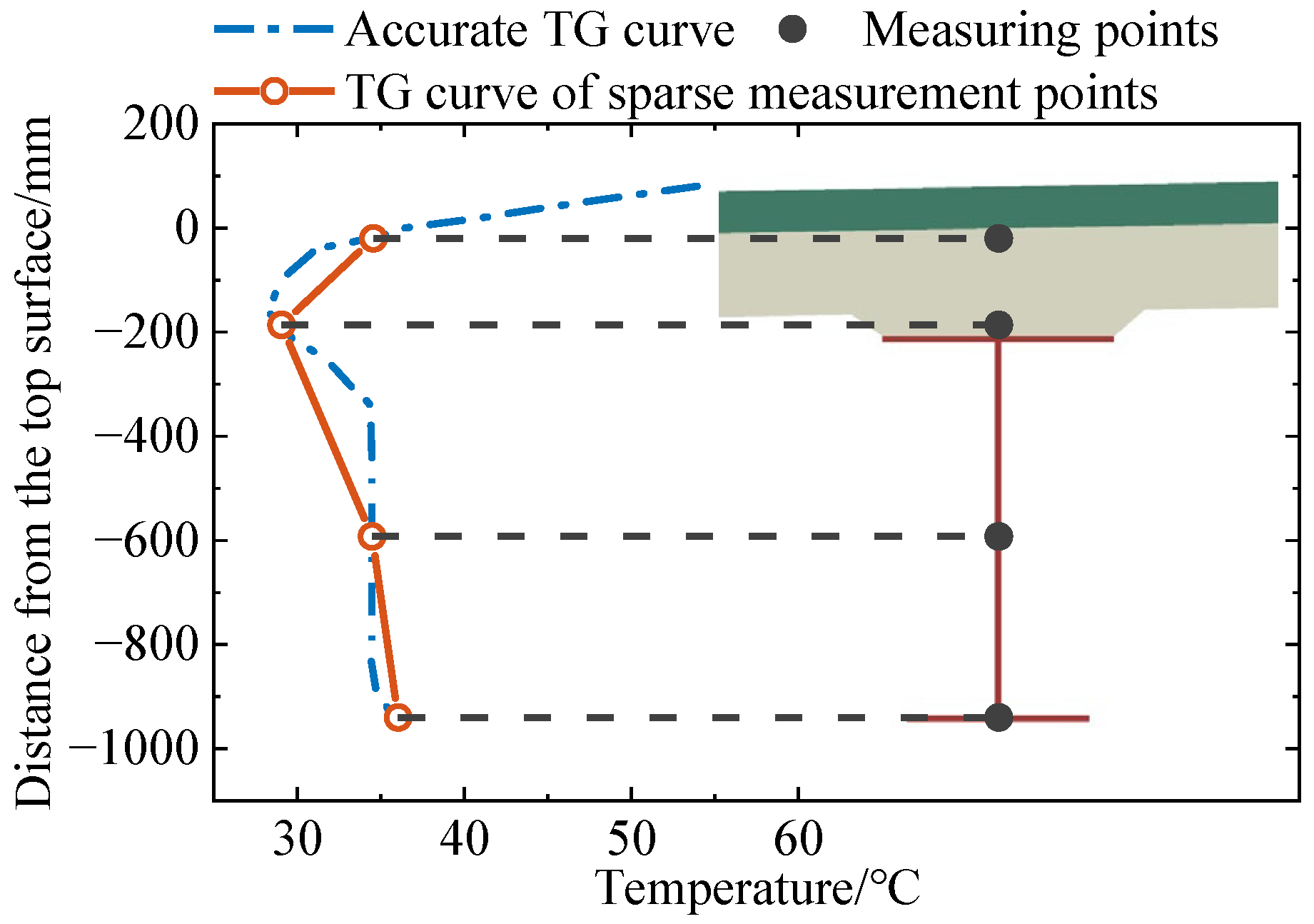
The temperature measuring points’ number and distances are unreasonable in a large amount of actual bridge temperature experiments. In most studies, the measuring points are arranged at equal distances, whereas in a few studies, the measuring points are arranged with variable distance. However, the distance of the measuring points is relatively random, lacks theoretical support, and the location of the measuring points often cannot cover the local extreme temperature points of the structure. Consequently, capturing the maximum TG of the structure is difficult.

(2)

The distribution of measuring points on different paths is the same, and the difference in the distribution modes of TTG at different depths and VTG at different offset distances are not considered. Thus, the TG data collected in the test cannot truly reflect the actual TG at different positions of the structure.

(3)

The method of arranging measuring points according to the statistical rule of measured temperature data has the problems of the long measuring period, high cost, and sparse arrangement of measuring points. Moreover, after a more reasonable arrangement is obtained through long-term statistical analysis, no more temperature measuring points can be added inside the concrete or closed steel beam.

To overcome the above problems, this paper proposes a total least squares improved piecewise Douglas–Peucker algorithm (TLS-IPDP) for the temperature measuring point arrangement of steel-concrete composite beams. The finite element (FE) model verified by experiments is used as a supplement to the long-term structural temperature measurement data. Based on the earlier numerical calculation, the most adverse TG curves and annual hourly TG curves under different paths are given for the following two typical steel-concrete composite beams (steel plate and steel box composite beams). Then, by thinning the curve and extracting feature points with the TLS-IPDP algorithm, the arrangement of temperature measuring points with a reasonable variation of distance in the longitudinal and transverse direction is optimized. The research results can provide a reference for the optimized arrangement of temperature measuring points in the design, construction control, and SHM of steel-concrete composite beams. They will also lay a foundation for the fine analysis of the structural temperature field and temperature effect.

2. Basic Theory of TLS-IPDP Algorithm

In the actual structure temperature test, if the temperature sensor size is sufficiently small and can be densely arranged on the path without considering space limitations and economic cost, then an accurate TG curve can be obtained by connecting the temperature measurement point data in straight lines as shown in Figure 1. However, the actual layout of temperature sensors is often sparse, and the TG curve obtained by connecting the data of measurement points in straight lines may not contain local peak values, resulting in a large deviation between the gradient of measured data and the real gradient. The key problem to be solved in this paper is how to convert the dense measurement points into sparse measurement points while preserving the feature points, to obtain a practical measurement point arrangement scheme while ensuring the accuracy of the measured TG curve. TTG and VTG are two important forms of temperature distribution, and the current national specifications for the structure temperature field, also take the vertical, and horizontal gradient as main indicators. The purpose of this paper is to obtain the temperature measurement point arrangement scheme which can reasonably collect the structure’s temperatures and reflect the overall temperature distribution characteristics of the structure. Therefore, both the induction of FEM calculation results and the data basis of the TLS-IPDP algorithm in the following are carried out in the form of TTG and VTG.

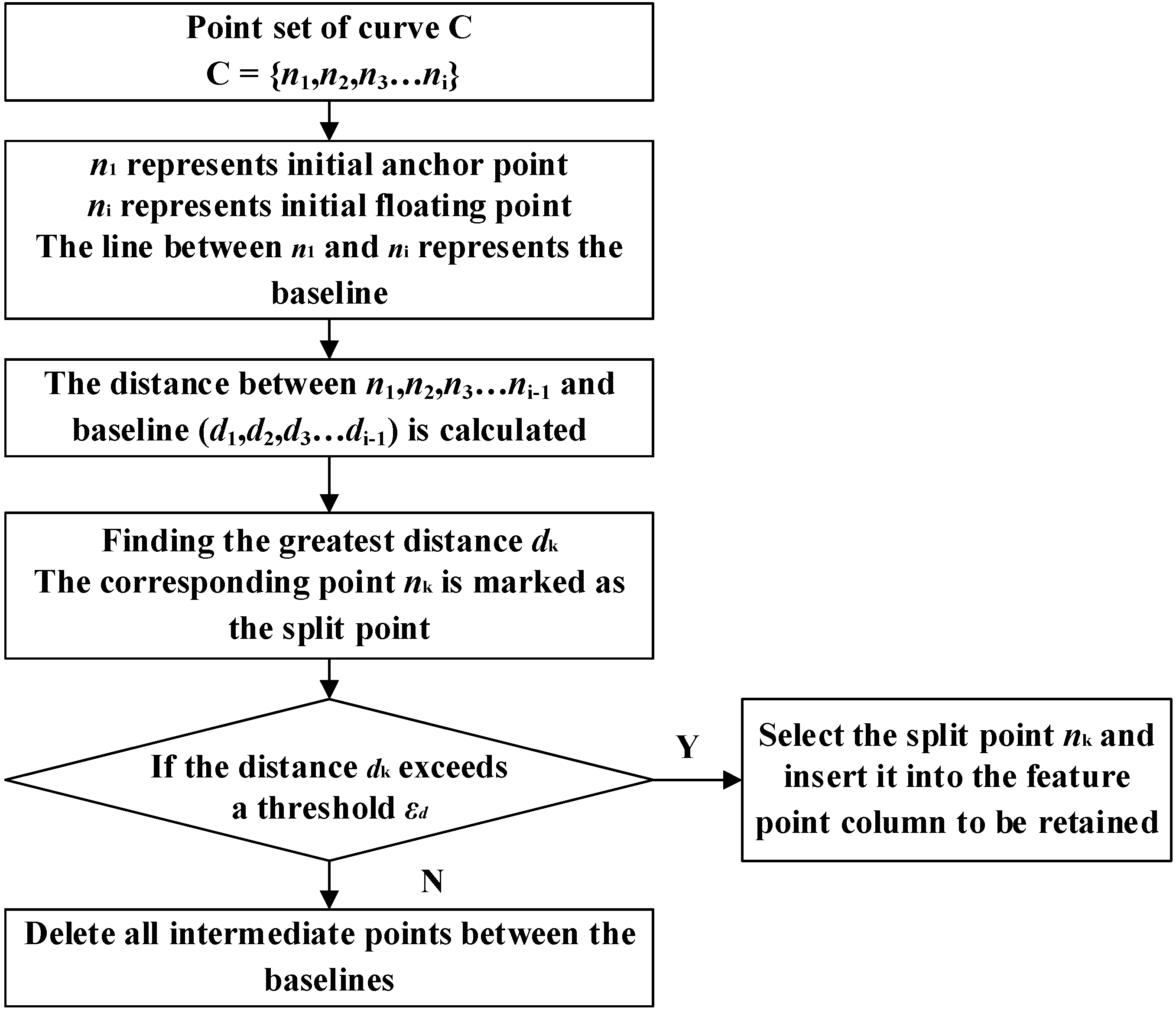
2.1. Douglas–Peucker Algorithm

On the premise of ensuring the key local features of the curve, the transformation from dense measurement points to sparse measurement points requires curve thinning while retaining the key features of the curve. Douglas and Peucker proposed the 2D curve morphological simplification method which uses global recursive operations to screen the main feature points that can reflect the local morphology of the curve in the complex curve point series [22,23]. The basic flow of the classic DP algorithm is shown in Figure 2, and if the floating-point is not adjacent to the anchor point at this time, the 2D point series is divided into 2 parts with the split point as the boundary, repeating the process until no new split points are generated.

As a lossy compression algorithm, the DP algorithm still has some defects:

(1)

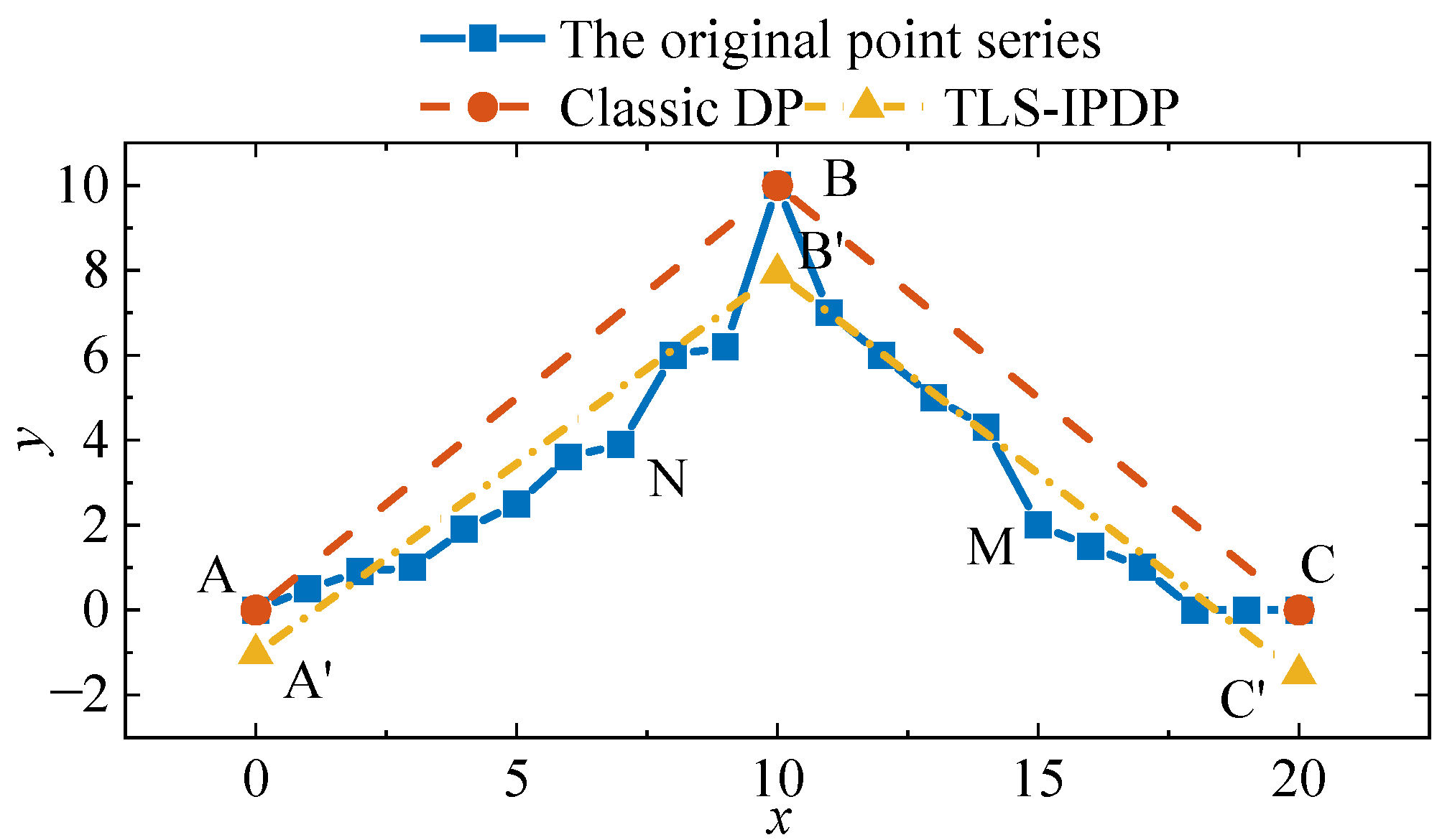
The loss of important feature points could easily occur in parts with large curvature; meanwhile, the retention of non-feature points could easily happen in parts with small curvature, thus affecting the compression effect.

(2)

Steel-concrete composite beams have a specific material boundary, and measuring points need to be arranged in specific locations as required; the feature points to be preserved cannot be specified artificially in the DP algorithm.

(3)

Considering the constraints of structural size and economic cost, the optimal number of sensors in steel-concrete composite beams should be calculated. However, in the DP algorithm, the number of feature points to be retained cannot be manually specified but can only be controlled by the threshold ${\epsilon }_d$.

2.2. Design of TLS-IPDP Algorithm

Aiming at the above three defects, this paper proposes a TLS-IPDP algorithm, which can be applied to optimize the temperature feature point series. Its main improvements are as follows:

(1)

The total least square method is introduced. If $d_k\le {\epsilon }_d$, the total least square linear fitting is performed for all intermediate points between baselines. Otherwise, the split point $n_k$ is selected and inserted into the feature point series to be retained.

(2)

Before the search for the first split point, the retention points of the curve were manually specified according to the actual situation, and the feature point series was divided into multiple segments by the retention points. Then, the split points were searched for multi-segments.

(3)

The random search method is used to automatically search the appropriate threshold value according to the artificially specified retention feature point number n. The algorithm automatically updates the number of retention points to a value in the range of $\left[n-5,n+5\right]$ and recalculates until the threshold ${\epsilon }_d$ meets the requirements so that the original feature point series is thinned and the updated retention feature point number is closest to $n$.

Different from the conventional least-squares method, the basic principle of the total least squares method is as follows: For point series $\mathit{P}=\left\{p_1,p_2,p_3,\cdots ,p_i\right\}$, its coordinates are $\left\{(x_1,y_1),(x_2,y_2),(x_3,y_3),\cdots ,(x_i,y_i)\right\}$; then, its geometric center coordinate can be expressed as

$$\overline{x}=\frac{1}{n}{\displaystyle \sum _{i=1}^n{x}_i},\overline{y}=\frac{1}{n}{\displaystyle \sum _{i=1}^n{y}_i}$$

(1)

The equation of the line can be written as $y-\overline{y}=k\left(x-\overline{x}\right)$, and the centralized data vector is

$$\begin{array}{l}\mathit{X}=\left[x_1-\overline{x},x_2-\overline{x},\cdots x_n-\overline{x}\right]\\ \mathit{Y}=\left[y_1-\overline{y},y_2-\overline{y},\cdots y_n-\overline{y}\right]\end{array}$$

(2)

The conventional least square method considers only the noise in $\mathit{Y}$, whereas the total least square method considers both the noise in $\mathit{X}$ and $\mathit{Y}$. If ${\mathit{\epsilon }}_x$ represents the error in $\mathit{X}$, ${\mathit{\epsilon }}_y$ represents the error in $\mathit{Y}$, then, $\left(\mathit{X}-{\mathit{\epsilon }}_x\right)k=\mathit{Y}-{\mathit{\epsilon }}_y$. An appropriate slope $k$ is selected to minimize the Frobenius norm of the total error $\mathit{E}=\left[{\mathit{\epsilon }}_x,{\mathit{\epsilon }}_y\right]$, that is, minimize

$$\mathit{\xi }={‖\mathit{E}‖}_F^2=\mathrm{Tr}\left[{\mathit{E}}^{\mathrm{T}}\mathit{E}\right]$$

(3)

Let the augmented matrix $\widehat{\mathit{X}}$ and the augmented vector $\widehat{\mathit{k}}$, respectively, be

$$\begin{array}{l}\widehat{\mathit{X}}=\left[\mathit{X},\mathit{Y}\right]\\ \widehat{\mathit{k}}={\left[k,-1\right]}^{\mathrm{T}}\end{array}$$

(4)

According to the Rayleigh quotient principle, the cost function of the total least squares can be expressed as

$$\mathit{\xi }=\widehat{\mathit{k}}\mathit{P}\widehat{\mathit{k}}/\left({\widehat{\mathit{k}}}^{\mathrm{T}}\widehat{\mathit{k}}\right),\mathit{P}={\widehat{\mathit{X}}}^{\mathrm{T}}\widehat{\mathit{X}}$$

(5)

When the augmented vector $\widehat{\mathit{k}}=\eta {\mathit{v}}_0$, the cost function of the total least square method takes the minimum value, where v₀ is the eigenvector that corresponds to the minimum eigenvalue of the matrix P, and $\eta$ satisfies that the last component of $\widehat{\mathit{k}}$ is equal to −1.

The Figure 3 compares the thinning results of the point series of the classic DP algorithm with that of the TLS-IPDP algorithm in this paper. A threshold ${\epsilon }_d$ is assumed to exist so that only the split point B is retained on the curve ABC, and the maximum distances d_N and d_M from the new splitting point N and M to the line AB and BC are both less than the threshold ${\epsilon }_d$. The thinning result of the DP algorithm is the straight lines AB, BC, and the thinning result of the TLS-IPDP algorithm is A′B′, B′C′. The optimized result of the TLS-IPDP algorithm is closer to the original point series.

3. Optimization Method of Temperature Measuring Point Layout Based on TLS-IPDP

For the arrangement of temperature measuring points of steel-concrete composite beams, apart from reasonable selection of the distance between measuring points according to the actual TG distribution mode of the structure, the following four problems should also be considered:

(1)

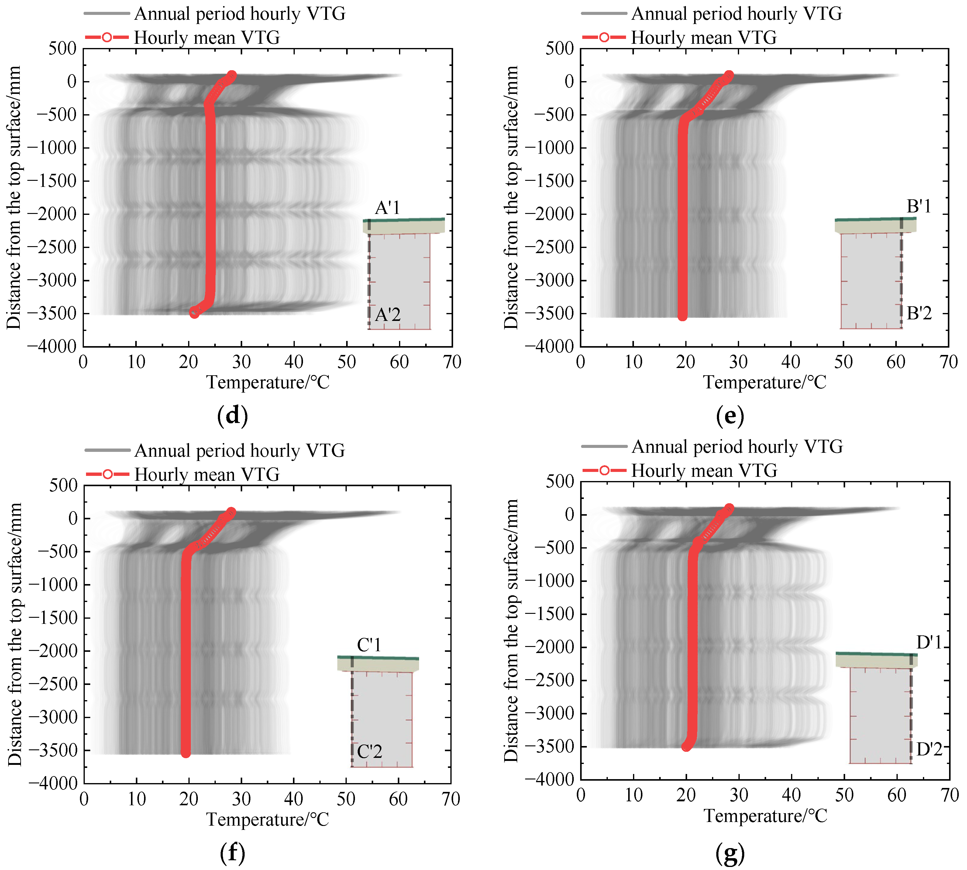
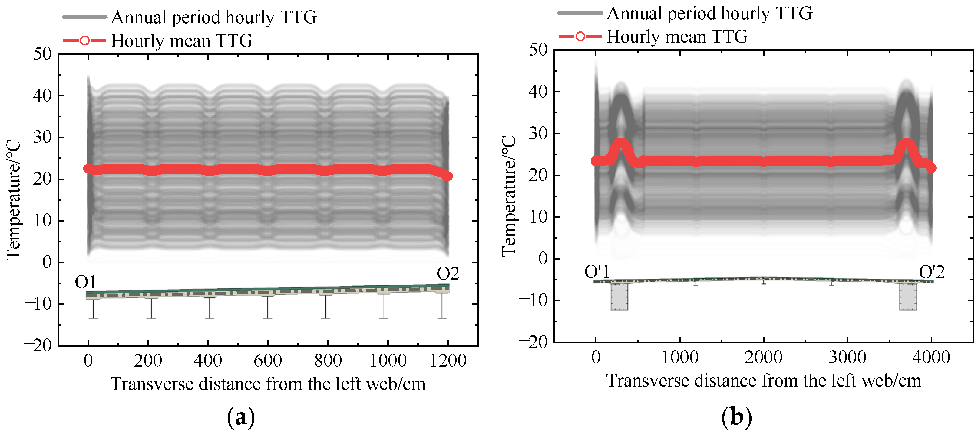
Owing to the influence of bridge orientation and geographical location, solar radiation and convective heat transfer with uneven time-varying characteristics lead to differences in TG distribution modes and temperature extremes between transverse paths with different depths and vertical paths with different offsets [12,24].

(2)

Owing to the difference in thermophysical parameters between steel and concrete, the vertical arrangement of temperature measuring points should be discussed separately for steel beam and concrete bridge slab.

(3)

Conventional steel-concrete composite beams have two typical structural forms: steel plate composite beam (Type I) and steel box composite beam (Type II). The temperature distributions of open and closed sections are different.

(4)

Statistical analysis of the long-term measured temperature data of the structure to obtain its distribution rule can reasonably guide the arrangement of temperature measuring points. However, for a real bridge that has been tested for a long time, adding extra temperature measuring points inside the concrete and closed steel beam is often impossible.

Therefore, based on the above four problems, this paper adopts the process shown in Figure 4 to generate the arrangement scheme of temperature measuring points under specified conditions. This method is illustrated and verified by two engineering examples with Types I and II construction forms.

4. Case-Studies

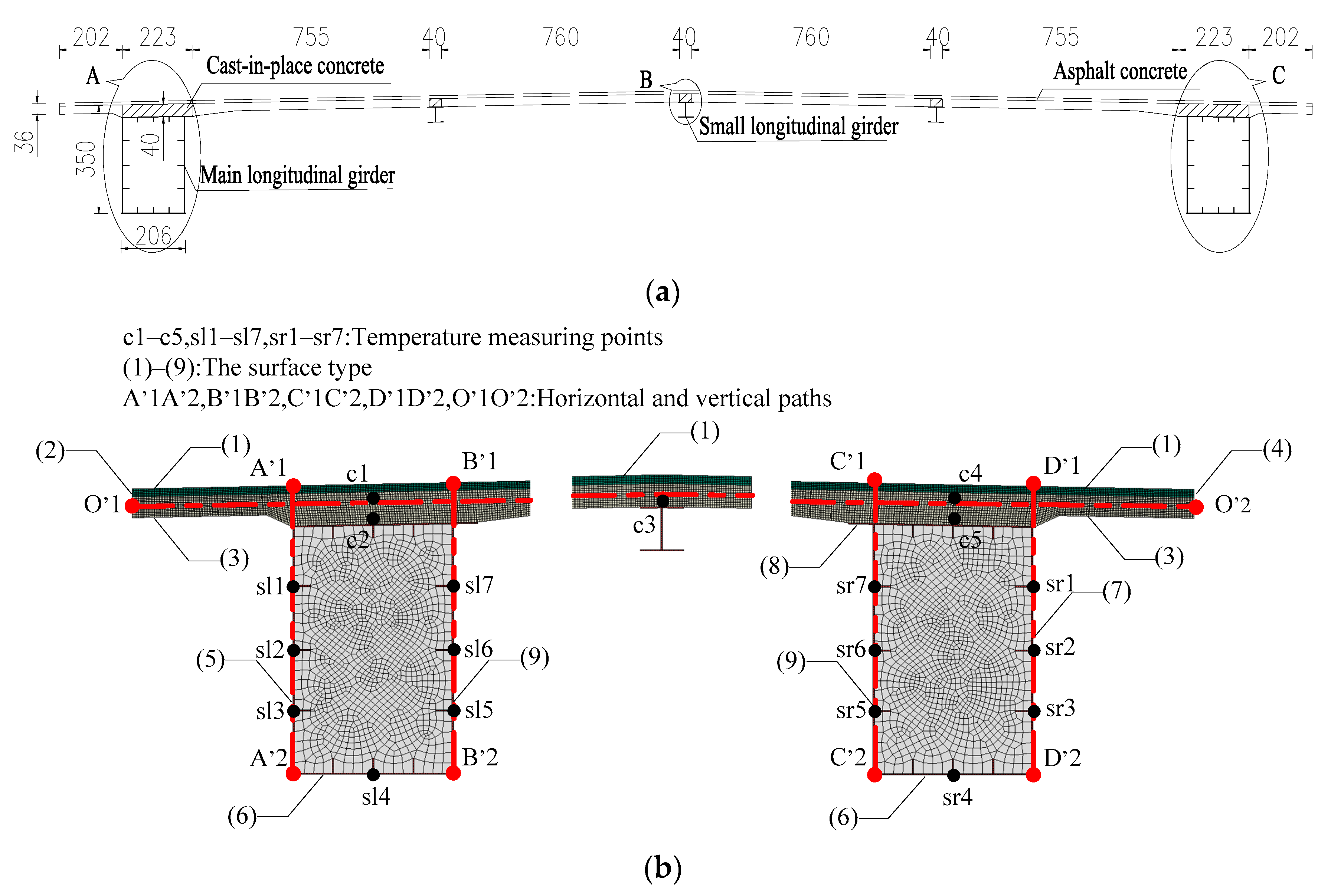
4.1. Engineering Description

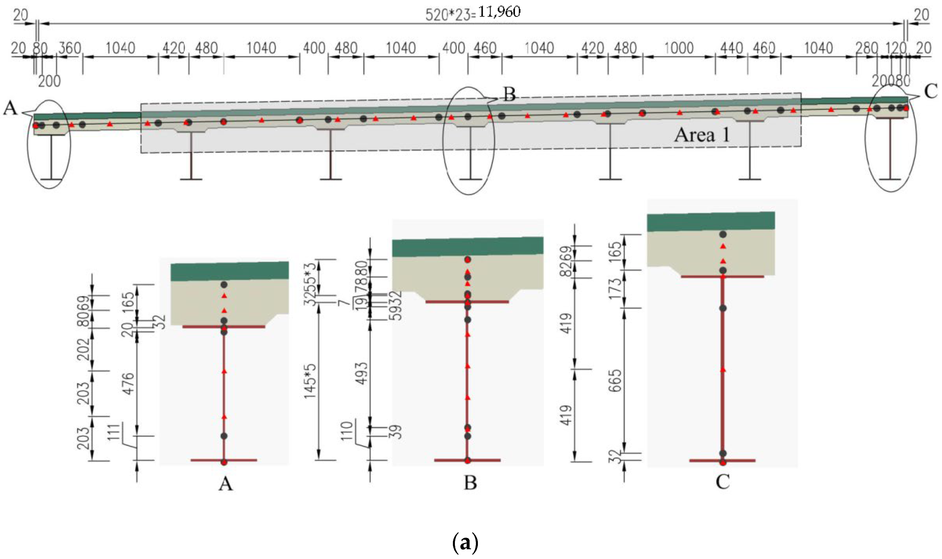
4.1.1. Type I: Steel Plate Composite Beam

A single-span stiffened steel truss suspension bridge is located at 119.610° E, 28.334° N, at 571.100 m above sea level. Figure 5 shows the main geometric parameters of the section, location of temperature measuring points C1–C4-S1–S4, paths, and surface types (1)–(9).

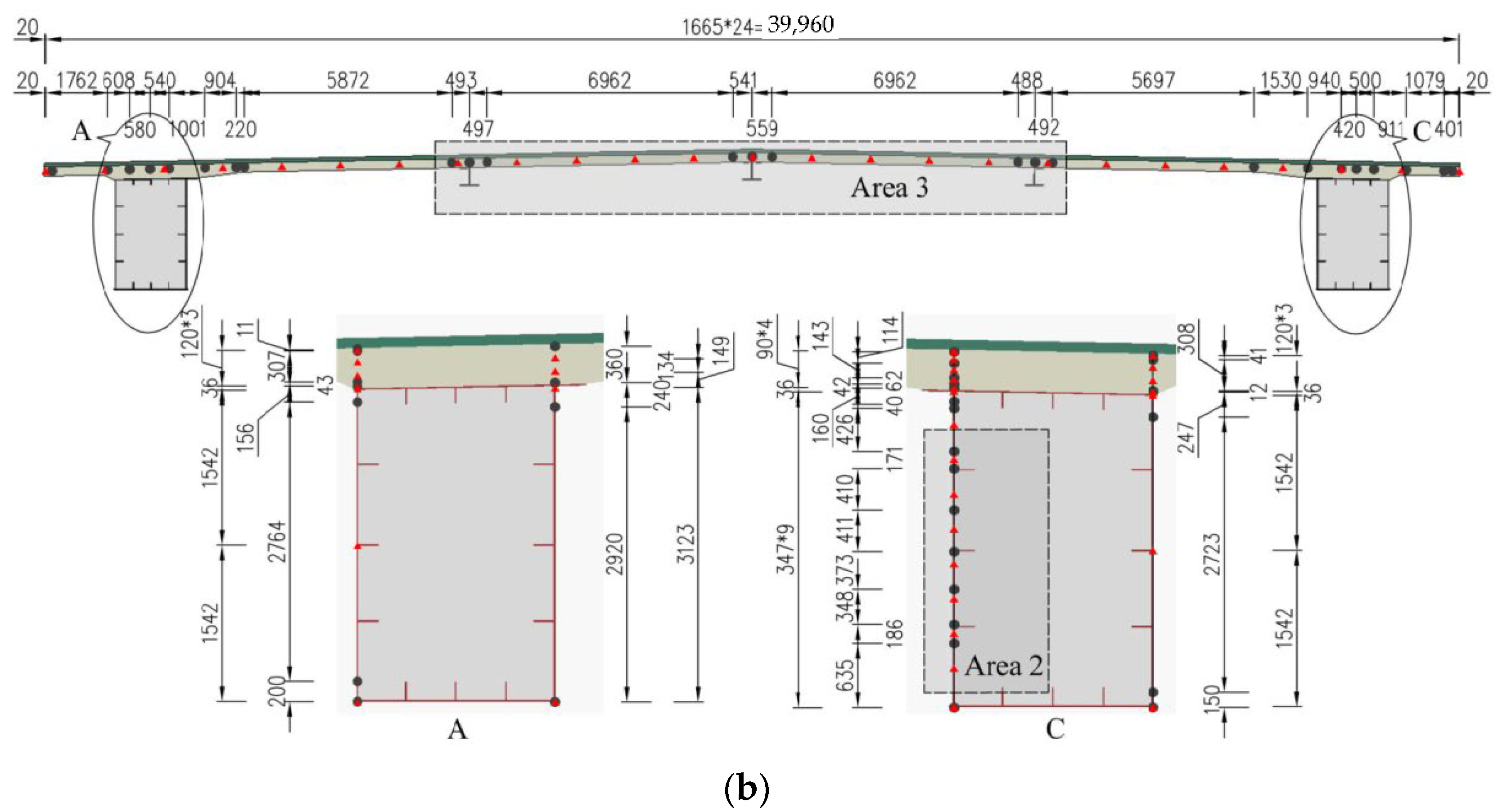
4.1.2. Type II: Steel Box Composite Beam

The main span of a 480 m composite girder cable-stayed bridge is located at 104.694° E, 28.779° N, and 313.717 m above sea level. The middle span is a steel box composite beam. Figure 6 shows the main geometric parameters of the section, location of temperature measuring points C1–C5-SL1–SL7-SR1–SR7, paths, and surface types (1)–(9).

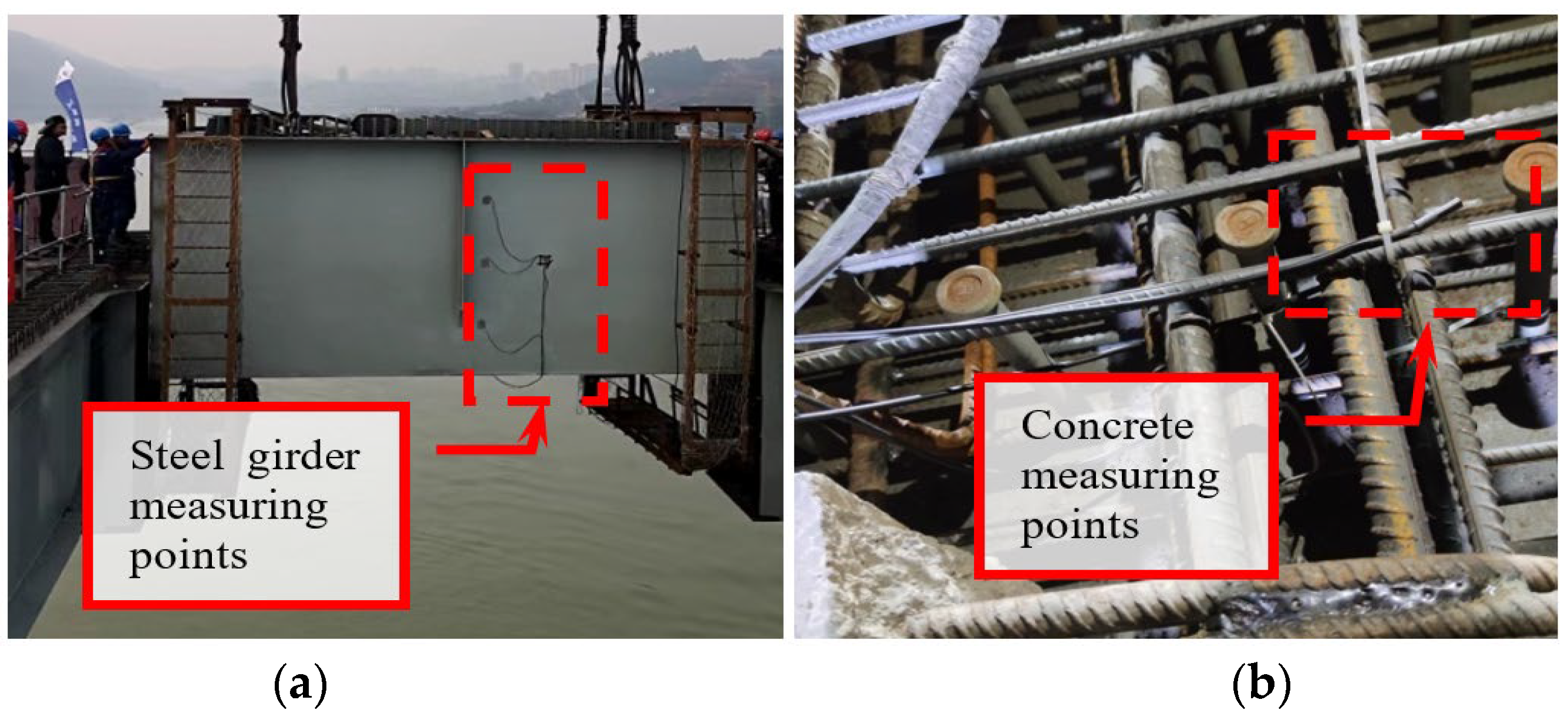
4.1.3. Selection and Arrangement of Temperature Sensors

This study adopts the 16-bit digital pulse structure with dedicated temperature sensors with a wide temperature measurement range (−50, 135) °C (Figure 7), and the temperature measurement accuracy can reach ±0.3 °C at room temperature. Measuring points are arranged for the vertical and transverse paths of Types I and II. Figure 5b and Figure 6b show the paths and positions, and Figure 8 shows the partial measuring points in the real bridge. It is worth noting that Figure 7 is intended to show the appearance of the sensors used in this paper, rather than placing multiple sensors in nearly the same location at the same time.

4.2. Calculation of Structural Annual Periodic Hourly Temperature Field Considering the Geographical Location and Meteorological Condition Difference

Based on the temperature measurement of the two types of steel-concrete composite beams in Section 4.1, the long-term temperature data at the location of the measuring points were obtained. However, compared with the size of the whole bridge, the arrangement of measuring points remained sparse, unable to effectively reflect the VTG and TTG, and unable to obtain the temperature data in the operation state before the completion of the bridge. Numerical simulation, as a convenient method to study the temperature field of bridges, has slowly developed from the early 1D difference method to 3D time-varying temperature field simulation based on the general finite element simulation platform [25,26] after years of improvement and has been extensively verified [12,16,27,28]. To obtain the annual period hourly temperature data of the full section in advance, based on heat transfer theory and considering the differences in geographical location and meteorological conditions, the thermal transfer FEM calculation is carried out on the structure, and the correctness of the calculation results is verified by the measured data.

4.2.1. FEM Modeling

2D FEM models of heat transfer including a pavement layer were established respectively for the above Types I and II steel-concrete composite structures. The global seed size of the two models is approximately 20 mm, and a dense grid is carried out for the junction of concrete and steel beams to ensure the accuracy of the calculation results of the contact positions of different materials. In particular, for the section of type II, heat transfer elements are also established for the air-filled (gray grid) parts to accurately consider the heat transfer in the box cavity, as shown in Figure 5b and Figure 6b.

2D heat transfer FEM models including pavement layer were established for the above Types I and II steel-concrete composite structures. A total of 9499 nodes and 8517 DC2D4 elements were in the Type I model and 43,542 nodes, 39,882 DC2D4 elements, and 13 DC2D3 elements were in the Type II model. The global seed size of the two models is approximately 20 mm, and a dense grid is carried out for the junction of concrete and steel beams to ensure the accuracy of the calculation results of the contact positions of different materials. In particular, for the section of type II, heat transfer elements are also established for the air filled in it to accurately consider the heat transfer in the box cavity. Figure 5b and Figure 6b show the local detailed grid of the two models (the gray part in Figure 5b is the grid for air). In the FE simulation of the box girder temperature field, the influence of air in the box chamber on the structure temperature field was usually ignored. To calculate the temperature field more accurately, the air in the closed chamber was approximately simulated by two-dimensional heat transfer elements [29]. The air elements and the steel elements were connected by the nodal coupling method, so that the heat conduction between the air and the steel, and the radiation heat transfer between the closed chamber formed by the steel were considered simultaneously.

4.2.2. Thermophysical Properties of Materials

Based on the actual test of material properties and the literature [30,31,32,33],

Table 1. Thermophysical parameters of main materials.

Model Type	Material	ρ/kg·m−3	Thermal Conductivity/W·m−1·K−1	Specific Heat/J·kg−1·°C−1
I	Concrete	2549	1.70	920
	Asphalt concrete	2100	1.05	1168
	Steel	7850	53.2	460
II	Concrete	2549	1.70	960
	Asphalt concrete	2360	1.05	1198
	Steel	7850	53.2	480
	Air	See Table 2	0.023	1081

shows the material thermophysical parameters. Considering that air density is affected by temperature, humidity, and air pressure, the density of dry air at different temperatures under standard atmospheric pressure is selected to be input into the FEM models [34]. Additionally, the air density is designated as a function of temperature, which is calculated automatically by the program (

Table 2. Dry air density at standard atmospheric pressure.

t/°C	0	10	20	30	40	50	60	70	80
$\rho$/kg·m−3	1.2928	1.2471	1.2046	1.1649	1.1277	1.0926	1.060	1.0291	1.000

).

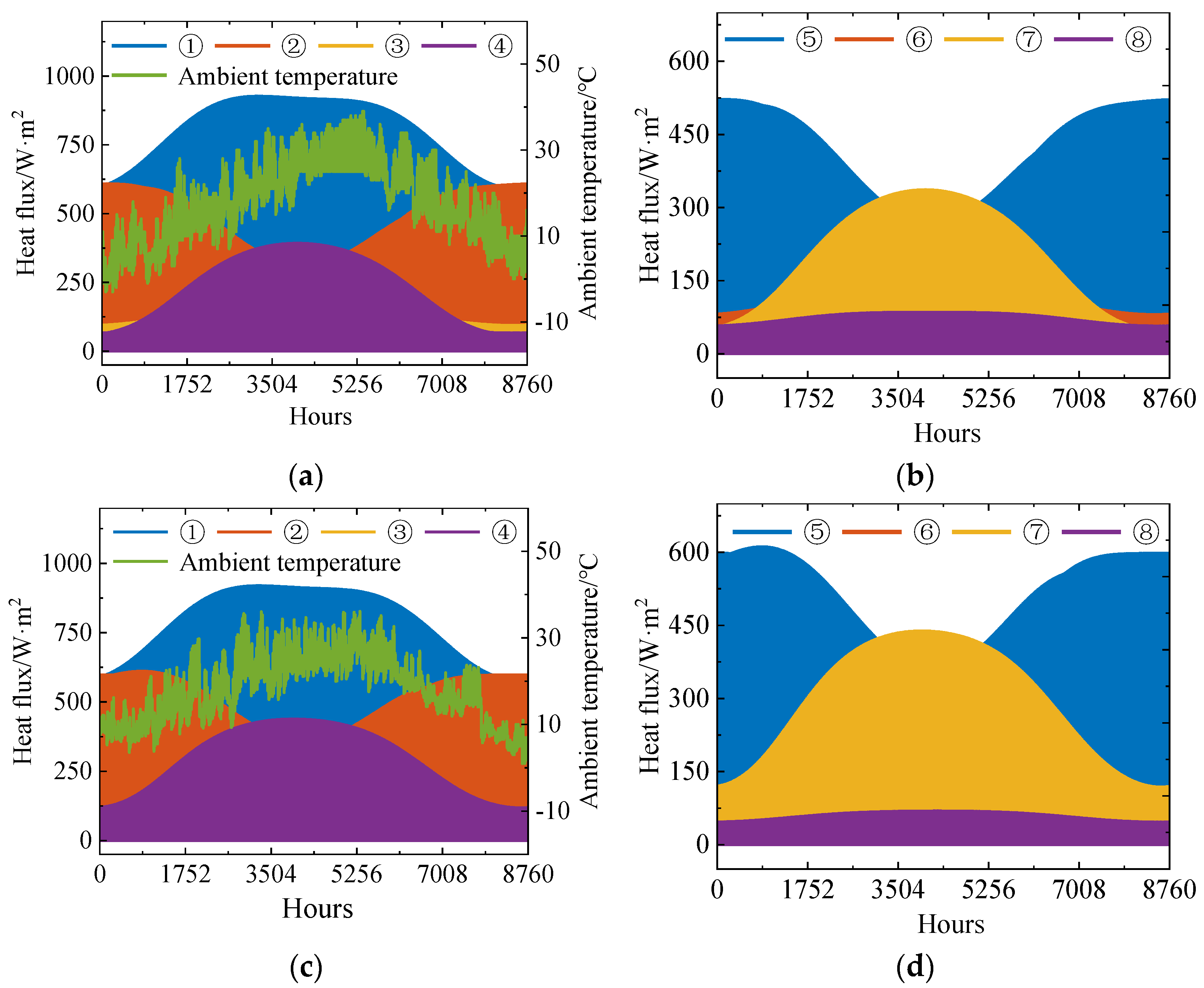
4.2.3. Boundary Conditions and Initial Temperature Field

For large bridge structures, it is difficult to accurately test the temperature on each boundary. Therefore, the second type of boundary condition was adopted in this paper, and it requires the known heat flux on the boundary which can be calculated by Equations (7)–(9).

q(t) is used to represent the heat flux of the known object boundary, namely, the second boundary condition:

$${\left.k\frac{\partial T}{\partial n}\right|}_{\mathrm{\Gamma }}=q\left(t\right)=q_c\left(t\right)+q_r\left(t\right)+q_s\left(t\right)$$

(6)

where $n$ represents the outer normal direction of boundary $\mathrm{\Gamma }$, q_c(t) represents the heat flux of convective heat transfer between object boundary and surrounding fluid, q_r(t) represents the heat flux of thermal radiation heat transfer, and q_s(t) represents the heat flux of solar radiation heat transfer.

The calculation formulas of q_c(t), q_r(t), and q_s(t) are as follows:

$$q_c\left(t\right)=h\left[T_a\left(t\right)-T\right]$$

(7)

$$q_r\left(t\right)=\epsilon C_0\left\{{\left[T_0+T_a\left(t\right)\right]}^4-{\left[T_0+T\right]}^4\right\}$$

(8)

$$q_s\left(t\right)=A_s\left(I_{D\varphi }+I_{d\beta }+I_{\gamma \beta }\right)$$

(9)

where T_a(t) represents the ambient temperature and is a function of time t [35]. According to the extreme value of daily temperature, the sine function is used to simulate the daily temperature process [36]. h represents the surface heat transfer coefficient, which is related to structure orientation and wind speed. Based on the literature and correction with experimental results [37],

Table 3. Calculation parameters of boundary conditions.

Parameters		Model
		I	II
h/m·s−1	Asphalt Concrete top surface (1)	14.33	14.11
	Concrete lower surface (3)	9.83	10.51
	Concrete vertical surface (2)(4)	11.33	11.54
	Steel beam lower surface (6)(8)	11.05	12.85
	Steel beam vertical surface (5)(7)(9)	13.29	13.17
$\epsilon$	Asphalt Concrete	0.95	0.95
	Concrete	0.9	0.9
	Steel	0.6	0.6
C0/W·m−2·K−4		5.67 × 10−8
$A_s$	Asphalt Concrete	0.90	0.90
	Concrete	0.70	0.75
	Steel	0.60	0.75

shows the convective heat transfer coefficient of the structural surface (1)–(9) shown in Figure 5 and Figure 6. ε is the material emissivity, C₀ is Stefen–Boltzman constant, and T₀ = 273.15, whose purpose is to convert °C into K. A_s is the short-wave radiation absorption rate of the structure surface. We refer to other scholars’ studies for specific parameter calculations [38], which will not be described here.

Table 3 and Figure 9 present the calculation results of the above boundary parameters and heat flux of some surfaces.

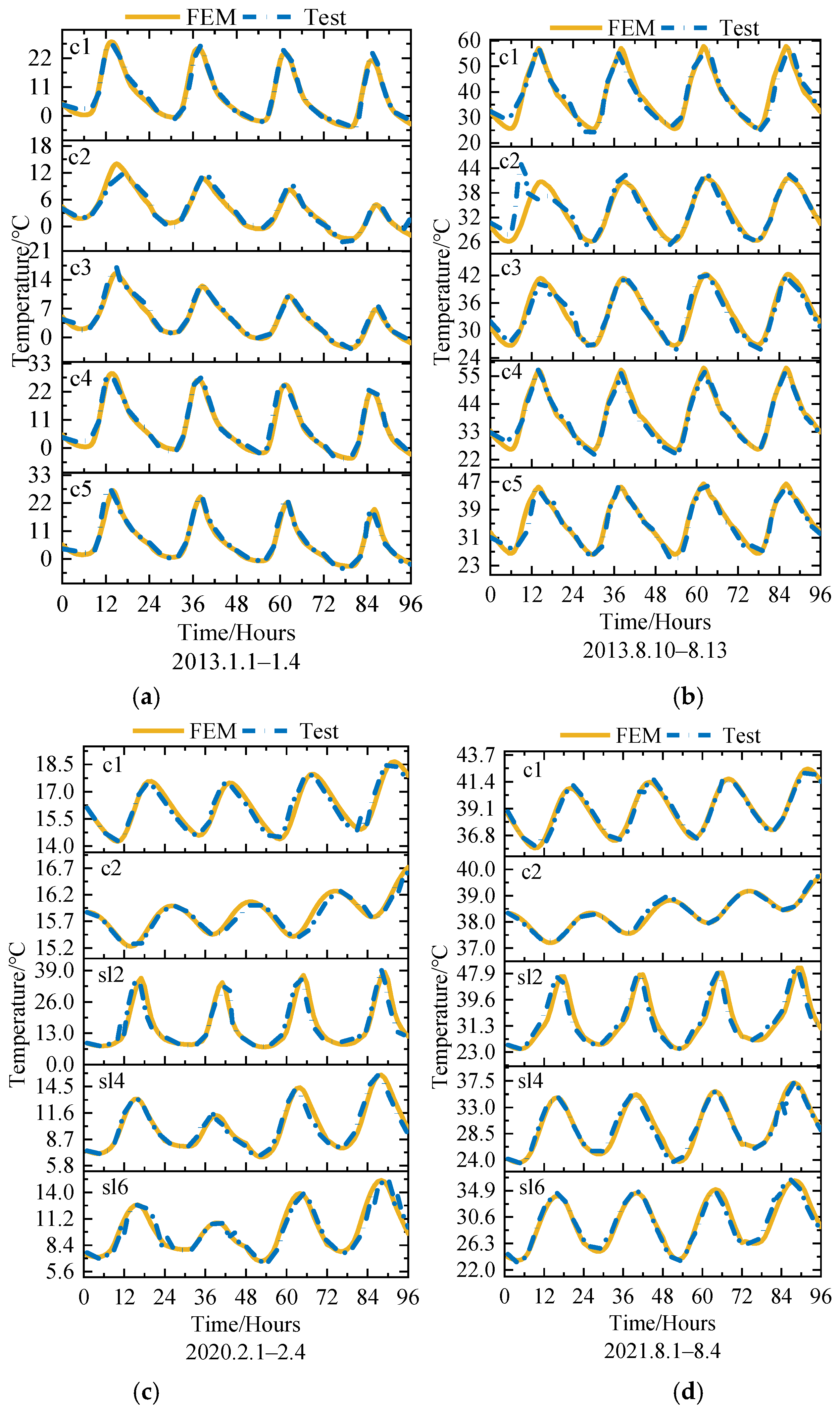
4.2.4. Verification of Calculation Results

The measured data are used to verify the annual period hourly temperature field FEM calculation results of the two models. For all the sensors deployed in the two types of cases (the specific positions are shown in Figure 5 and Figure 6), there is a large amount of test data for a long time which is difficult to reflect in the manuscript. Therefore, only the measured data of some measuring points are given in this paper to illustrate the correctness of the FEM results; the figures below only show the comparison between the measured and FEM values in typical low-temperature and typical high-temperature periods. Figure 10 shows that in the two kinds of model of FEM calculation results, the estimated temperatures tally with the measured temperatures, and the temperature variation of each measuring point in the FEM calculation is consistent with the actual test results. Therefore, the following VTG and TTG curves can be accurately extracted by the established FE models of the two types of steel-concrete composite beams.

4.3. Feature Extraction of TG Curve

4.3.1. VTG

The arrangement of VTG measuring points in the structure should cover most extreme cases. Meanwhile, the location of measuring points should be as close as possible to the feature points of the actual VTG curve at different times to reduce the deviation of the measured results. Therefore, the feature points of the VTG curves in different vertical paths of the two types of models are extracted by considering the characteristics of the most adverse VTG and the VTG distribution at different moments in the annual period hourly temperature FEM calculation, respectively. Considering that the two types of steel-concrete composite beams are located in China, the most adverse VTG is stipulated in the Chinese code as shown in Figure 11 [39].

The year 2013/2020 hourly temperature fields of the two models were calculated (Case I is for the whole year 2013, and case II is for the whole year 2020.), and the temperature values at the corresponding positions of T₁ and T₂ on the vertical path were extracted; the temperature bases T₁ and T₂ were obtained after normalization. As seen in Figure 11, the vertical position of the structure corresponding to the temperature base T₁ and T₂ is fixed. When T₁ − T₂ is the largest, its vertical gradient is the largest. Figure 11 illustrates the maximum value of T₁ − T₂ per month.

As seen in Figure 12, the maximum value of T₁ − T₂ of the Type I model appeared on path B1B2, and that of the Type II model appeared on path C′1C′2. Figure 13 shows the most adverse VTG curve at the time when the maximum value of T₁ − T₂ appeared in the two models. (The maximum value of T₁ − T₂ in the Type I model appears at 14:00 on 17 May 2013, and that in the Type II model appears at 16:00 on 26 April 2020).

By comparing the most adverse VTG curves in Figure 11 and Figure 13, the VTG curve in the central area of the concrete slab in Figure 13 can be found to have reverse bending, and its temperature is lower than that of the steel beam. The latter results in a difference from the three-stage VTG curve given in Figure 11. Therefore, the characteristics of the VTG curve in the Chinese code are different from the actual most adverse VTG, and the VTG given in Figure 13 can better reflect the characteristics of the most adverse VTG of the structure.

All feature points (red circular marks in Figure 13) of the most adverse VTG curves with negative ordinates in Figure 13a,b were recorded. The ordinate of these feature points means that, on the premise of the same number of temperature measuring points and feature points, if the temperature measuring points are arranged according to the vertical position of feature points, the most adverse VTG curve of the structure can be accurately fitted from the test data of the measuring points.

The frequency of the most adverse VTG is very low in the actual SMH data. The SMH system typically collects the temperature data under the daily temperature cycle in the entire life cycle of the structure and evaluates the structural safety by integrating other data such as strain, displacement, and acceleration. If the temperature measurement points are only arranged according to the feature points of the most adverse VTG curve, the collected data may omit too many local extreme values of the real VTG distribution of the structure under the daily temperature cycle. This scenario leads to the deviation of the temperature effect calculation based on the TG and affects the accuracy of the structure state assessment. Therefore, statistical analysis of annual period hourly VTG in all vertical paths is needed to fit the hourly mean VTG curve with the minimum error of temperature distribution at each moment and to extract its feature points.

Annual period hourly VTG calculation results of all vertical paths of the two types of models were extracted and written as a matrix group $T^V=\left\{T_1^V,T_2^V\right\}$ of nodes on each path. For the Type I model, a matrix group $T_1^V=\left\{T_{A1A2}^{49\times 8760},T_{B1B2}^{57\times 8760},T_{C1C2}^{60\times 8760}\right\}$ exists and a matrix group $T_2^V=\left\{T_{A{}^{\prime }1A{}^{\prime }2}^{174\times 8784},T_{B{}^{\prime }1B{}^{\prime }2}^{176\times 8784},T_{C{}^{\prime }1C{}^{\prime }2}^{176\times 8784},T_{D{}^{\prime }1D{}^{\prime }2}^{174\times 8784}\right\}$ exists for the Type II model. A curve with 99% transparency was drawn for each column of the matrix and was superimposed. The mean value of each row of each matrix in the matrix group (i.e., the mean value of the temperature at the same time every day of each path in a year) was calculated to generate the hourly mean VTG vector group $t^V=\left\{t_1^V,t_2^V\right\}$. For the Type I model, a vector group $t_1^V=\left\{t_{A1A2}^{49\times 1},t_{B1B2}^{57\times 1},t_{C1C2}^{60\times 1}\right\}$ exists and a vector group $t_2^V=\left\{t_{A{}^{\prime }1A{}^{\prime }2}^{174\times 1},t_{B{}^{\prime }1B{}^{\prime }2}^{176\times 1},t_{C{}^{\prime }1C{}^{\prime }2}^{176\times 1},t_{D{}^{\prime }1D{}^{\prime }2}^{174\times 1}\right\}$ exists for the Type II model. Figure 14 provides the above data.

In Figure 14, each hourly VTG curve is highly transparent. After they are superimposed in the same coordinate system, the darker the color is, the more times the same or similar temperature occurs at this position, which reflects the frequency difference of annual period hourly VTG. Considering that the hourly VTG curve’s color (gray curves) at the junction of the steel girder and the concrete plate is darker, the hourly mean VTG curve (red curves) has a large gradient in the concrete area and a small gradient in the steel beam area. It means that the actual temperature measuring points can be arranged in steel beams with fewer measuring points, whereas concrete parts require extra measuring points to obtain a more accurate temperature distribution. All feature points of the hourly mean VTG curves with negative ordinates in Figure 13 (red circular mark) were recorded. The coordinates of these feature points mean that, on the premise of the same number of temperature measuring points and feature points, if the temperature measuring points are arranged according to the vertical position of feature points, the deviation between the measured VTG and the real VTG curves at each time in the annual cycle would be the smallest.

4.3.2. TTG

As for the arrangement of structure transverse temperature measurement points, considering that the TTG is largely affected by the bridge direction and shelter, among others, the most adverse TTG is thus not considered here except for the annual period hourly mean TTG curves under the transverse path to extract feature points. (Figure 5b and Figure 6b present the paths, wherein the transverse path O1O2 of Type I model contains 601 nodes, and the transverse path O′1O′2 of Type II model contains 1997 nodes. The paths can contain additional nodes if a smaller grid size is adopted).

In the same way, as in Section 4.3.1, annual period hourly TTG calculation results of all transverse paths of the two types of models were extracted and written as a matrix group $T^T=\left\{T_1^T,T_2^T\right\}$ of nodes on each path. For the Type I model, a matrix $T_1^T=T_{O1O2}^{601\times 8760}$ exists and a matrix $T_2^T=T_{O{}^{\prime }1O{}^{\prime }2}^{1997\times 8784}$ exists for the Type II model. A curve with 99% transparency was drawn for each column of the matrix and was superimposed. The mean value of each column of each matrix in the matrix group (i.e., the mean value of the temperature at the same time every day of each path in a year) was calculated to generate the hourly mean TTG vector group $t^T=\left\{t_1^T,t_2^T\right\}$. For the Type I model, a vector $t_1^T=t_{O{}^{\prime }1O{}^{\prime }2}^{601\times 1}$ existed, and a vector $t_2^T=t_{O{}^{\prime }1O{}^{\prime }2}^{1997\times 1}$ for the Type II model. Figure 15 provides the above data.

Similar to Figure 14, Figure 15 also reflects the frequency difference of the annual period hourly TTG. Combined with annual period hourly TTG curves (gray curves) and hourly mean TTG curves (red curve), the gradient of the two types of models near the left and right sides of the transverse path is easily seen as large. Therefore, in the arrangement of measuring points, additional measuring points should be used for the part with a larger gradient, whereas fewer measuring points should be used for the part with a smaller gradient.

All feature points of the hourly mean TTG curves in Figure 15 (red circular marks) were recorded.

4.4. Generation of TG Curve Thinning and Measurement Point Layout Optimization Scheme Based on TLS-IPDP

In Section 4.3, the feature points of VTG and TTG curves were extracted according to the FE calculation results. However, in practice, temperature measuring points could not be arranged so densely on corresponding paths. Therefore, the TLS-IPDP algorithm was used to thin the above curves and retain key feature points to obtain a practical measuring point optimal arrangement scheme.

The actual temperature measuring points are assumed to be arranged under the following restrictions: (1) temperature measuring points should be arranged at the interface of steel and concrete materials. (2) No more than 5 concrete temperature measurement points and no more than 10 steel temperature measurement points are in a single vertical path. No more than 25 temperature measurement points exist in a single transverse path. Additional measuring points should be arranged in areas with large temperature gradients on the left and right sides.

The number of retained feature points after thinning is the number of temperature measuring points to be arranged, and the coordinates of retained feature points after the optimization are the layout positions of temperature measuring points as shown in Figure 16.

Table 4. Statistical results of the number of measuring points.

Parts of the Structure	Number of Measuring Points
	Type I Model				Type II Model
	A1A2	B1B2	C1C2	O1O2	A′1A′2	B′1B′2	C′1C′2	D′1D′2	O′1O′2
Concrete	2	4	2	9 + 15 (Area 1)	4	2	5	4	16 + 9 (Area 3)
Steel	4	6	3	/	3	2	3 + 7 (Area 2)	3	/
Total	6	10	5	24	7	4	15	7	25

shows the statistical results of the number of measuring points to be arranged for steel and concrete. Combined with Figure 16 and Table 4, the TLS-IPDP algorithm proposed in this paper effectively achieves curve optimization under restricted conditions by manually specifying splitting points and automatically updating thresholds and the total number of target feature points. Compared with the redundant data in the original curve, the TLS-IPDP algorithm largely simplifies the curve. For the vertical path, the number of feature points thinned from a single VTG curve is at most 10, and the number of feature points thinned from a single TTG curve is at most 25 for the transverse path. For paths O1O2, C′1C′2, and O′1O′2, multiple peaks and troughs occur because a steel-concrete interface (Area 1, Area 3) or stiffening rib (Area 2) exists along the path direction, and the TG caused by this feature is not large compared with the whole. If these three parts are ignored, the number of temperature measuring points can be further reduced. In addition, compared with the defect of the traditional arrangement of temperature measuring points that ignores the difference of TG in different paths and adopts the same equidistance arrangement for different paths, the TLS-IPDP algorithm considers the difference of TG mode in different paths and generates different variable-distance arrangements for measuring points in different paths, which make the fitting curve of the measured results closer to the actual TG.

Figure 16 shows the arrangement of measuring points for each path according to the thinning results (black circular marks). The thinning results of the B1B2 and C′1C′2 paths consider the synthesis of hourly mean VTG and the most adverse VTG curves. Meanwhile, considering that the actual structure could not accommodate temperature measuring points on the concrete surface, the points on the concrete surface in the thinning result were all offset to 20 mm along the internal direction, so that the measuring point arrangement in Figure 17 could be used for the actual temperature measuring point arrangement.

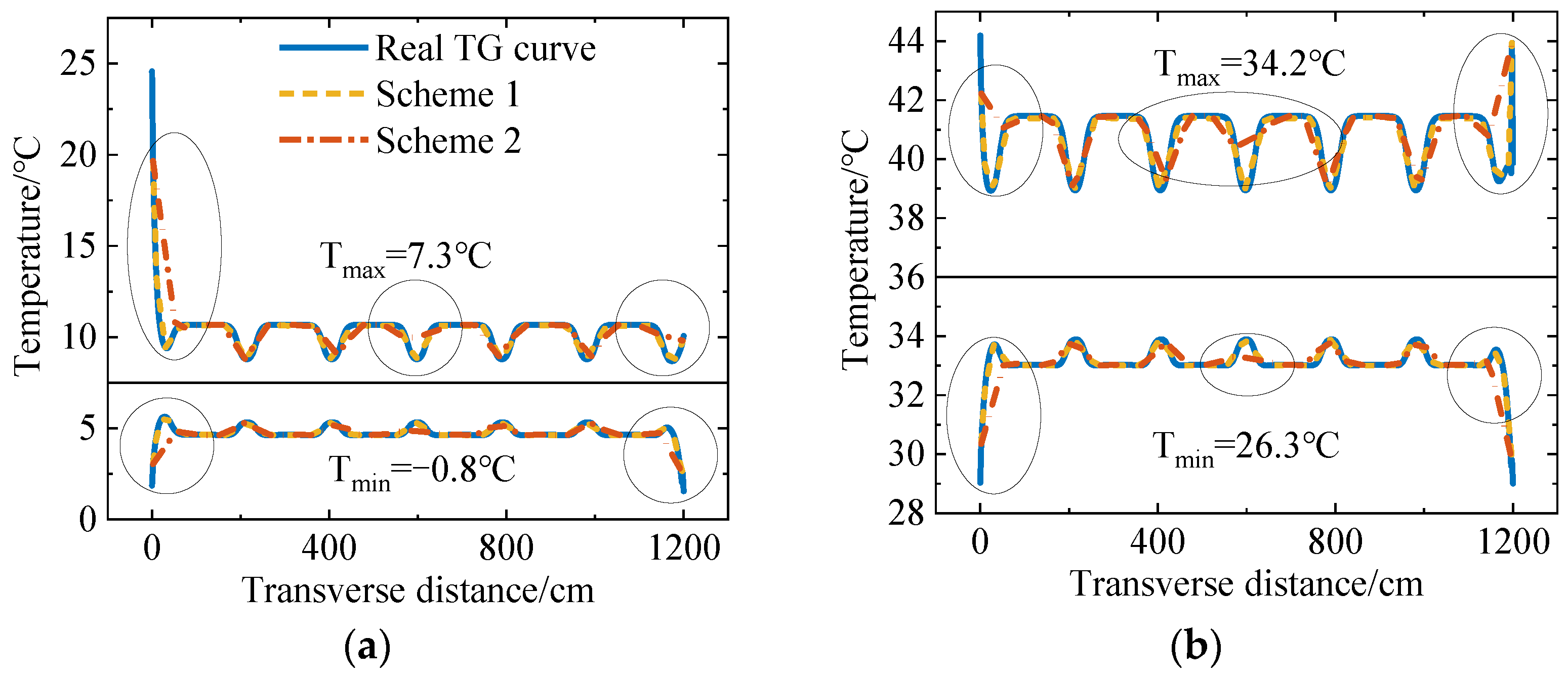
4.5. Comparison with Traditional Measuring Point Arrangement Scheme

To compare the measurement data difference between the temperature measuring point arrangement by TLS-IPDP and the traditional equal-distance arrangement, the temperature values of black point series and red point series of each path in typical periods of high and low temperatures were extracted.

Table 5. Typical periods of high and low temperatures.

Model Type	Temperature
	Low	High
I	16 January (Tmin = −0.8 °C, Tmax = 7.3 °C)	26 July (Tmin = 26.3 °C, Tmax = 34.2 °C)
II	27 December (Tmin = 1.0 °C, Tmax = 11.0 °C)	10 July (Tmin = 26.3 °C, Tmax = 36.1 °C)

T_min and T_max, respectively, represent the lowest and highest ambient temperatures of the day. Their fitted curves were compared with the real VTG and real TTG curves. Figure 18 shows the results. (Owing to space limitations, only the comparison results of paths B1B2, O1O2, C′1C′2, and O′1O′2 are given).

As seen from the figure, the TG curves obtained by the TLS-IPDP measuring point arrangement in this paper are significantly better than those obtained by traditional equidistance measuring point arrangements, and significant differences exist between them in the region with a large gradient (the part circled in Figure 17). The local temperature extremum is often not collected in the traditional equidistance measuring point arrangement, which leads to a great difference between the fitted TG curves and the real TG curves. In the TLS-IPDP method, the measurement points were more accurately set at the feature points of the real TG curve, and the local extreme values were captured so that the fitting curves given by the TLS-IPDP measuring point arrangement were closer to the real TG curves, and their trend was more consistent with the real curve.

5. Conclusions

To overcome the defects of the traditional temperature measuring point arrangement and generate a reasonable arrangement of temperature measuring points of steel-concrete composite beams based on theoretical support, this paper extracted the most adverse VTG curves and the hourly mean VTG and TTG curves by the results of heat transfer FEM verified by field tests. It then provides the arrangement scheme of temperature measurement points by the TLS-IPDP algorithm. The results show that:

(1)

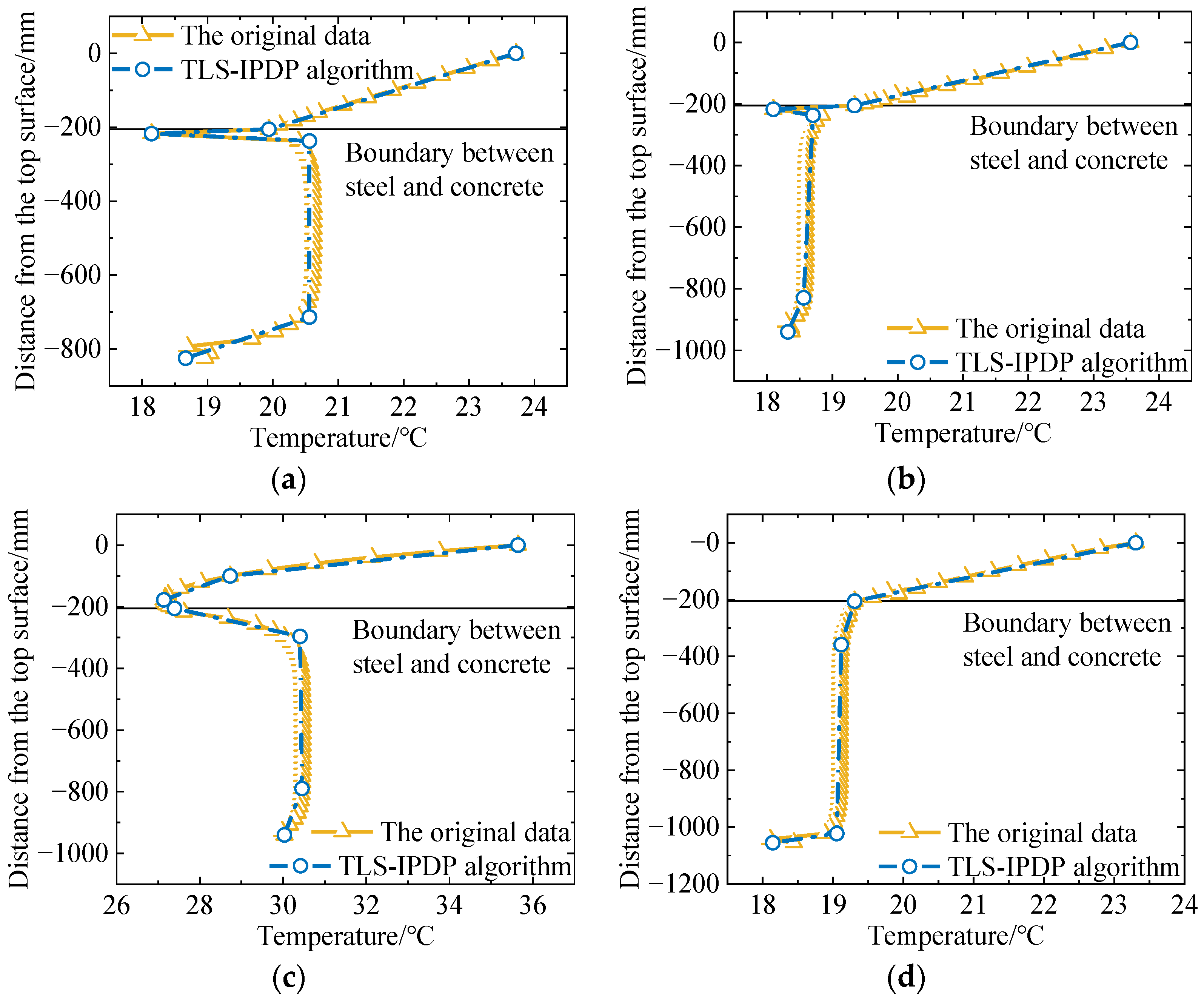
By improving the DP algorithm, the TLS-IPDP algorithm introduces the total least squares to enable a better approximation of the original data. Additionally, it has the function of artificially specifying the feature points to be retained and can automatically search the threshold according to the number of specified retained feature points.

(2)

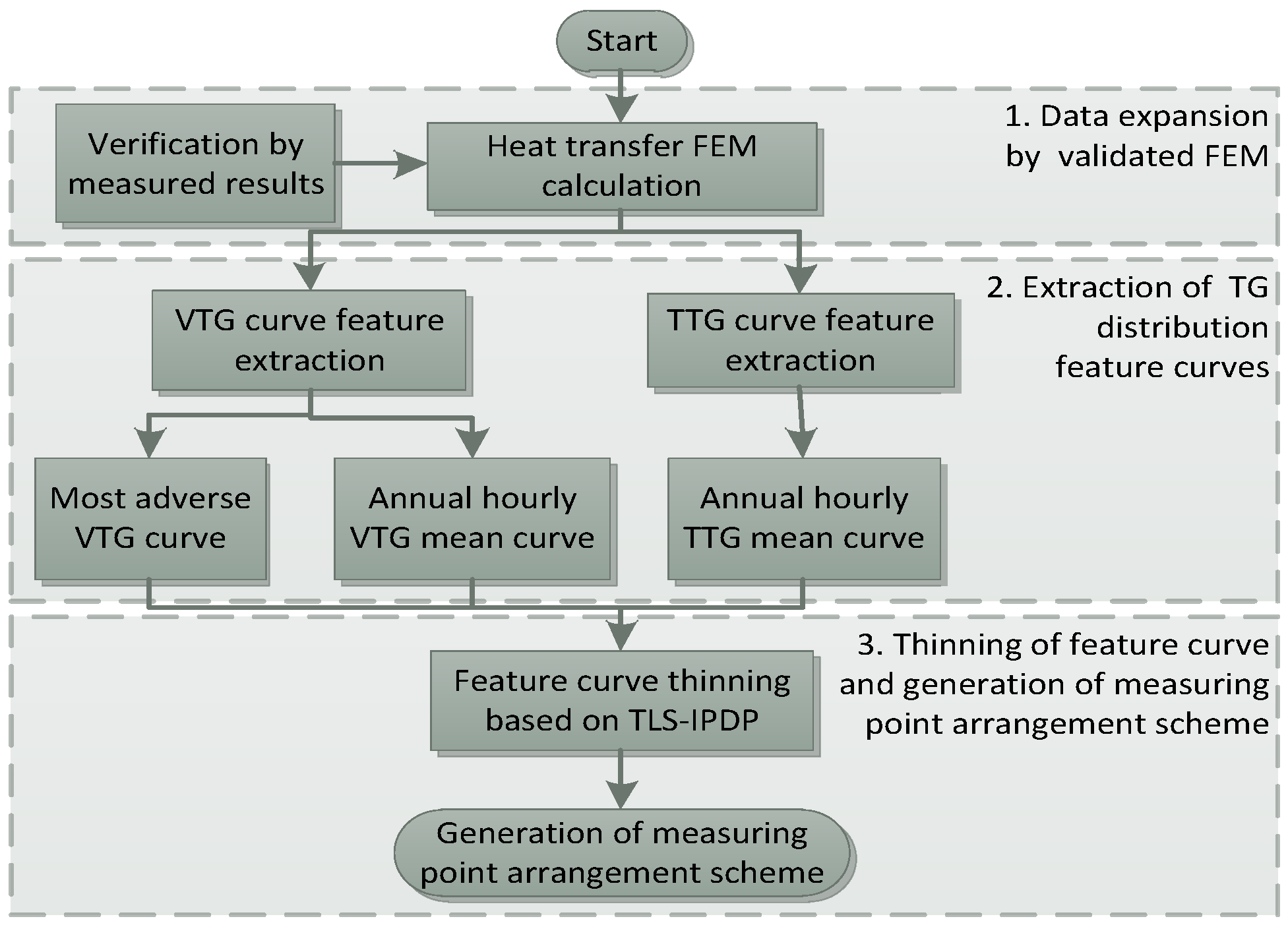
The calculated results of FEM based on heat transfer theory are quite consistent with the measured results. In addition, a more accurate structure TG distribution can be obtained through FEM calculation, which overcomes the defects of real bridge measurement methods such as long periods, high cost, sparse measurement points, and inability to increase internal measurement points.

(3)

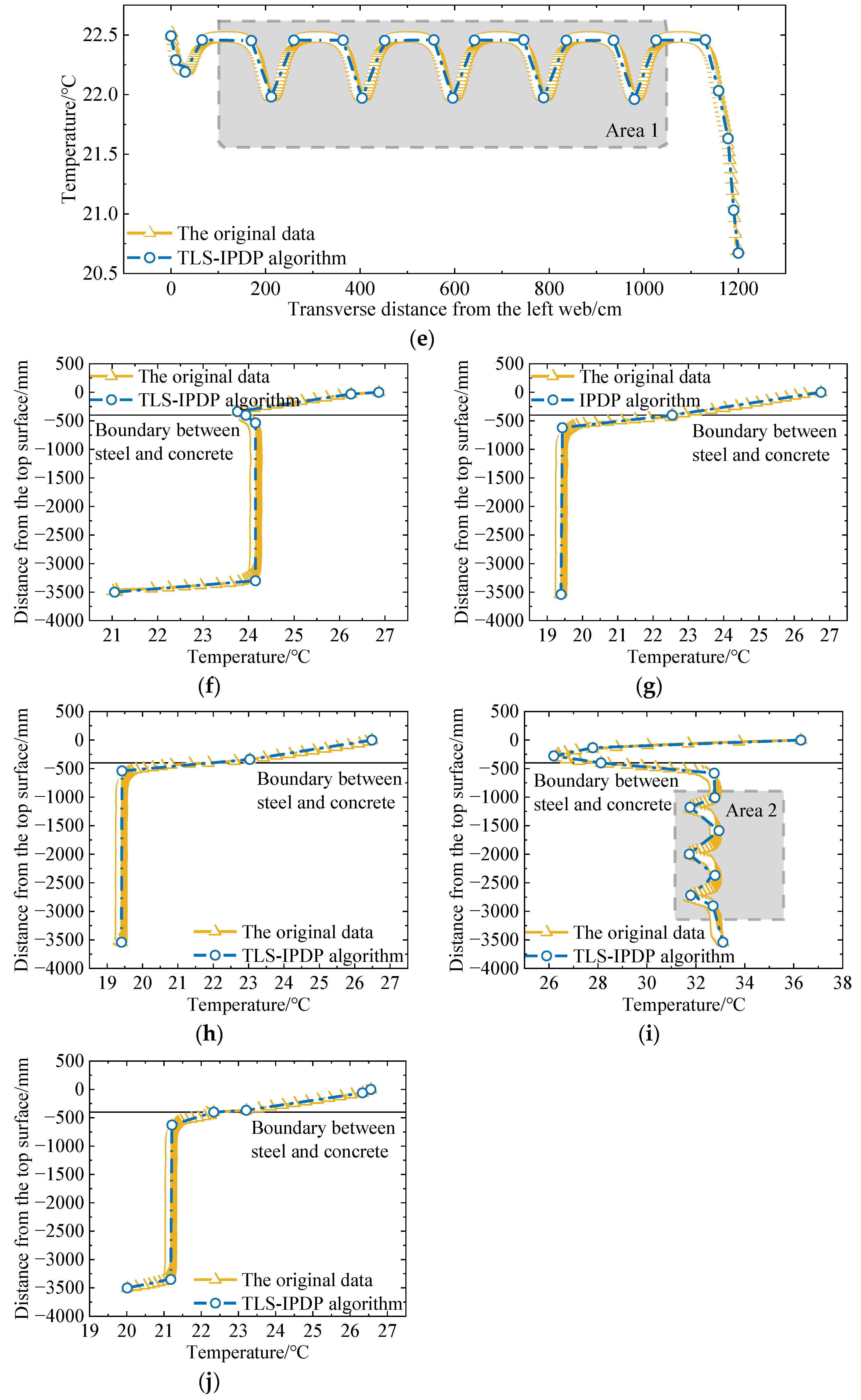
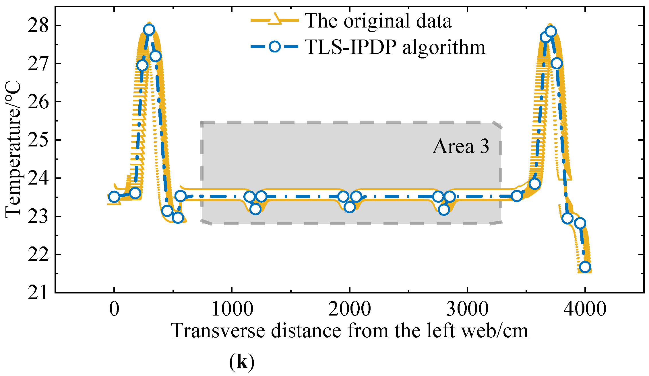
The TLS-IPDP algorithm proposed in this paper effectively realizes the thinning of original feature point columns under restricted conditions by manually specifying split points and automatically updating threshold values. The algorithm greatly simplifies the curve and compresses the redundant data. The maximum number of feature points after refining a single temperature curve for the vertical path is 10, and the maximum number of feature points after refining a single temperature curve for the horizontal path is 25. The effective optimization is achieved under the limitation of the number and accuracy of measuring points.

(4)

Using the TLS-IPDP algorithm combined with the results of FEM can generate a more reasonable temperature measuring point arrangement. Compared with the traditional equidistance temperature measuring point arrangement, the method in this paper considers the differences of TG modes under different paths and realizes the reasonable variable distance temperature measurement point arrangement of steel-concrete composite beams. The obtained TG curve is closer to the real TG distribution of the structure, and the error is smaller in the region with a larger gradient.

References

1. Liu, J.; Liu, Y.; Zhang, C.; Zhao, Q.; Lyu, Y.; Jiang, L. Temperature action and effect of concrete-filled steel tubular bridges: A review. J. Traffic. Transport. Eng. 2020, 7, 174–191. [Google Scholar] [CrossRef]
2. Liu, Y.; Liu, J. Review on temperature action and effect of steel-concrete composite girder bridge. J. Traffic. Transport. Eng. 2020, 20, 42–59. [Google Scholar]
3. Gottsäter, E.; Ivanov, O.L.; Molnár, M.; Crocetti, R.; Nilenius, F.; Plos, M. Simulation of thermal load distribution in portal frame bridges. Eng. Struct. 2017, 143, 219–231. [Google Scholar] [CrossRef]
4. Abid, S.R.; Mussa, F.; Tayşi, N.; Özakça, M. Experimental and finite element investigation of temperature distributions in concrete-encased steel girders. Struct. Control Health Monit. 2018, 25, e2042. [Google Scholar] [CrossRef]
5. Bao, Y.; Hoehler, M.S.; Smith, C.M.; Bundy, M.; Chen, G. Measuring three-dimensional temperature distributions in steel–concrete composite slabs subjected to fire using distributed fiber optic sensors. Sensors 2020, 20, 5518. [Google Scholar] [CrossRef]
6. Wang, J.; Ding, F.; Dai, J. Monitoring and Numerical Analysis for Construction Phase of a Steel-concrete Composite Continuous Box Girder Bridge. J. Highw. Transp. Res. Dev. 2006, 23, 91–94. [Google Scholar]
7. Zhou, G.; Yi, T. Thermal load in large-scale bridges: A state-of-the-art review. Int. J. Distrib. Sens. Netw. 2013, 9, 217983. [Google Scholar] [CrossRef]
8. Wang, D.; Tan, B.; Xiang, S.; Wang, X. Fatigue Crack Propagation and Life Analysis of Stud Connectors in Steel-Concrete Composite Structures. Sustainability 2022, 14, 7253. [Google Scholar] [CrossRef]
9. Huang, Y.; Zhang, Q.; Bao, Y.; Bu, Y. Fatigue assessment of longitudinal rib-to-crossbeam welded joints in orthotropic steel bridge decks. J. Constr. Steel Res. 2019, 159, 53–66. [Google Scholar] [CrossRef]
10. Cheng, Z.; Zhang, Q.; Bao, Y.; Deng, P.; Wei, C.; Li, M. Flexural behavior of corrugated steel-UHPC composite bridge decks. Eng. Struct. 2021, 246, 113066. [Google Scholar] [CrossRef]
11. Zhang, Q.; Ma, Y.; Cui, C.; Chai, X.; Han, S. Experimental investigation and numerical simulation on welding residual stress of innovative double-side welded rib-to-deck joints of orthotropic steel decks. J. Constr. Steel Res. 2021, 179, 106544. [Google Scholar] [CrossRef]
12. Xiang, S.; Wang, D.; Yang, L.; Tan, B. Study on the life cycle simulation method of the temperature field and temperature effect of a steel–concrete composite bridge deck system. Meas. Control 2021, 54, 1068–1081. [Google Scholar] [CrossRef]
13. Subramaniam, K.V.; Kunin, J.; Curtis, R.; Streeter, D. Influence of early temperature rise on movements and stress development in concrete decks. J. Bridge Eng. 2010, 15, 108–116. [Google Scholar] [CrossRef]
14. Chang, S.; Im, C. Thermal behaviour of composite box-girder bridges. Proc. Inst. Civ. Eng. Struct. Build. 2000, 140, 117–126. [Google Scholar] [CrossRef]
15. Wang, D.; Liu, Y.; Liu, Y. 3D temperature gradient effect on a steel-concrete composite deck in a suspension bridge with field monitoring data. Struct. Control Health Monit. 2018, 25, e2179. [Google Scholar]
16. Liu, J.; Liu, Y.; Jiang, L.; Zhang, N. Long-term field test of temperature gradients on the composite girder of a long-span cable-stayed bridge. Adv. Struct. Eng. 2019, 22, 2785–2798. [Google Scholar] [CrossRef]
17. Zhang, C.; Liu, Y.; Liu, J.; Yuan, Z.; Zhang, G.; Ma, Z. Validation of long-term temperature simulations in a steel-concrete composite girder. Structures 2020, 27, 1962–1976. [Google Scholar] [CrossRef]
18. Sakiyama, F.I.H.; Lehmann, F.; Garrecht, H. Structural health monitoring of concrete structures using fibre-optic-based sensors: A review. Mag. Concr. Res. 2021, 73, 174–194. [Google Scholar] [CrossRef]
19. Kim, J.-W.; Lee, C.; Park, S. Damage localization for CFRP-debonding defects using piezoelectric SHM techniques. Res. Nondestruct. Eval. 2012, 23, 183–196. [Google Scholar] [CrossRef]
20. Jabir, S.A.; Gupta, N.K. Condition monitoring of the strength and stability of civil structures using thick film ceramic sensors. Measurement 2013, 46, 2223–2231. [Google Scholar] [CrossRef]
21. Zhang, Q.; Zhang, D.; Cui, C.; Lao, W.; Qiu, S.; Miao, H.; Song, S. Fatigue Crack Detection Method Based on Ultrasonic-guided Waves for the Longitudinal Rib Butt Weld of Steel Decks. China J. Highw. Transp. 2022, 35, 101–112. [Google Scholar]
22. Zhao, L.; Shi, G. A method for simplifying ship trajectory based on improved Douglas–Peucker algorithm. Ocean Eng. 2018, 166, 37–46. [Google Scholar] [CrossRef]
23. Douglas, D.H.; Peucker, T.K. Algorithms for the reduction of the number of points required to represent a digitized line or its caricature. Cartogr. Int. J. Geogr. Inf. Geovis. 1973, 10, 112–122. [Google Scholar] [CrossRef] [Green Version]
24. Lee, J.-H.; Kalkan, I. Analysis of thermal environmental effects on precast, prestressed concrete bridge girders: Temperature differentials and thermal deformations. Adv. Struct. Eng. 2012, 15, 447–459. [Google Scholar] [CrossRef]
25. Tong, M.; Tham, L.; Au, F.; Lee, P. Numerical modelling for temperature distribution in steel bridges. Comput. Struct. 2001, 79, 583–593. [Google Scholar] [CrossRef]
26. Fan, J.; Liu, Y.; Liu, C. Experiment study and refined modeling of temperature field of steel-concrete composite beam bridges. Eng. Struct. 2021, 240, 112350. [Google Scholar] [CrossRef]
27. Wang, D.; Deng, Y.; Liu, Y.; Liu, Y. Numerical investigation of temperature gradient-induced thermal stress for steel–concrete composite bridge deck in suspension bridges. J. Cent. South Univ. 2018, 25, 185–195. [Google Scholar] [CrossRef]
28. Qinghua, Z.; Ma, Y.; Wang, B. Analysis of Temperature Field and Thermal Stress Characteristics for a Novel Composite Bridge Tower Catering for Plateau Environment. Bridge Constr. 2020, 50, 30–36. [Google Scholar]
29. Ma, Z.; Liu, J.; Liu, Y.; Lv, Y.; Zhang, G. Regional difference of value taking of effective temperature for steel-concrete composite girder bridges. J. Zhejiang Univ. 2022, 56, 909–919. [Google Scholar]
30. Noumowé, A.; Siddique, R.; Ranc, G. Thermo-mechanical characteristics of concrete at elevated temperatures up to 310 C. Nucl. Eng. Des. 2009, 239, 470–476. [Google Scholar] [CrossRef]
31. Adl-Zarrabi, B.; Boström, L.; Wickström, U. Using the TPS method for determining the thermal properties of concrete and wood at elevated temperature. Fire Mater. Int. J. 2006, 30, 359–369. [Google Scholar] [CrossRef]
32. Branco, F.A.; Mendes, P.A. Thermal actions for concrete bridge design. J. Struct. Eng. 1993, 119, 2313–2331. [Google Scholar] [CrossRef]
33. Krishnan, J.M.; Rajagopal, K. Triaxial testing and stress relaxation of asphalt concrete. Mech. Mater. 2004, 36, 849–864. [Google Scholar] [CrossRef]
34. Zhao, R. Air Conditioning, 4th ed.; China Architecture & Building Press: Beijing, China, 2009. [Google Scholar]
35. Wang, Y.; Zhan, Y.; Zhao, R. Analysis of thermal behavior on concrete box-girder arch bridges under convection and solar radiation. Adv. Struct. Eng. 2016, 19, 1043–1059. [Google Scholar] [CrossRef]
36. Dilger, W.H.; Ghali, A.; Chan, M.; Cheung, M.S.; Maes, M.A. Temperature stresses in composite box girder bridges. J. Struct. Eng. 1983, 109, 1460–1478. [Google Scholar] [CrossRef]
37. Tayşi, N.; Abid, S. Temperature distributions and variations in concrete box-girder bridges: Experimental and finite element parametric studies. Adv. Struct. Eng. 2015, 18, 469–486. [Google Scholar] [CrossRef]
38. Kim, S.-H.; Cho, K.-I.; Won, J.-H.; Kim, J.-H. A study on thermal behaviour of curved steel box girder bridges considering solar radiation. Arch. Civ. Mech. Eng. 2009, 9, 59–76. [Google Scholar] [CrossRef]
39. Wang, D.; Tan, B.; Wang, X.; Zhang, Z. Experimental study and numerical simulation of temperature gradient effect for steel-concrete composite bridge deck. Meas. Control 2021, 54, 681–691. [Google Scholar] [CrossRef]
Figure 1. Comparison of TG curves.
Sustainability 14 09787 g001
Figure 2. DP algorithm theory.
Sustainability 14 09787 g002
Figure 3. Comparison of DP algorithm and TLS-IPDP algorithm.
Sustainability 14 09787 g003
Figure 4. Flow chart of temperature measuring point arrangement of steel-concrete composite bridges based on TLS-IPDP.
Sustainability 14 09787 g004
Figure 5. Type I: Steel plate composite beam: (a) Steel plate composite beam bridge deck system (unit: cm); (b) Measuring point arrangement; surface types; local FE grids; and paths of areas A, B, and C.
Sustainability 14 09787 g005
Figure 6. Type II: Steel box composite beam: (a) Steel box composite beam (unit: cm); (b) Measuring point arrangement; surface types; local FE grids; and paths of areas A, B, and C.
Sustainability 14 09787 g006
Figure 7. Temperature sensors.
Sustainability 14 09787 g007
Figure 8. Arrangement of temperature measuring points: (a) Steel girder; (b) Concrete deck.
Sustainability 14 09787 g008
Figure 9. Surface heat flux and ambient temperature (Numbers ①–⑧ in the figure represent surface types, consistent with Figure 5 and Figure 6): (a,b) Type I model; (c,d) Type II model.
Sustainability 14 09787 g009
Figure 10. Comparison of FEM values and measured values: (a,b) Type I; (c,d) Type II.
Sustainability 14 09787 g010
Figure 11. Specific VTG of the Chinese code.
Sustainability 14 09787 g011
Figure 12. Maximum value of T1T2 per month: (a) Type I; (b) Type II.
Sustainability 14 09787 g012
Figure 13. Most adverse VTG curves along path B1B2, C′1C′2, and feature points located under the most adverse VTG: (a) Type I; (b) Type II.
Sustainability 14 09787 g013
Figure 14. Annual period hourly VTG and hourly mean VTG: (ac) Type I; (dg) Type II.
Sustainability 14 09787 g014aSustainability 14 09787 g014b
Figure 15. Annual period hourly TTG and hourly mean TTG: (a) Type I; (b) Type II.
Sustainability 14 09787 g015
Figure 16. Curve thinning results by TLS-IPDP for each path: (a) Path A1A2 (Annual period); (b) Path B1B2 (Annual period); (c) Path B1B2 (Most adverse); (d) Path C1C2 (Annual period); (e) Path O1O2 (Annual period); (f) Path A′1A′2 (Annual period); (g) Path B′1B′2 (Annual period); (h) Path C′1C′2 (Annual period); (i) Path C′1C′2 (Most adverse); (j) Path D′1D′2 (Annual period); (k) Path O′1O′2 (Annual period).
Sustainability 14 09787 g016aSustainability 14 09787 g016bSustainability 14 09787 g016c
Figure 17. Measuring point arrangement of each path (Unit: mm): (a) Type I; (b) Type II.
Sustainability 14 09787 g017aSustainability 14 09787 g017b
Figure 18. Comparison of fitting TG curve of schemes 1 and 2 and real TG curves in typical periods of high and low temperatures: (a) 16 January, path O1O2; (b) 26 July, path O1O2; (c) 16 January, path B1B2; (d) 26 July, path B1B2; (e) 27 December, path O′1O′2; (f) 10 July, path O′1O′2; (g) 27 December, path C′1C′2; (h) 10 July, path C′1C′2.
Sustainability 14 09787 g018aSustainability 14 09787 g018b