Abstract
The application of distributed fiber sensing technology in civil engineering has been developed to obtain more accurate and reliable information for structural health monitoring (SHM). With this sensing technique, high-density strain data are provided to benefit the stability and robustness in a closed-loop damage detection method which has not yet been investigated. To address this concern, a two-stage approach for structural damage detection combining a modal strain energy-based index (MSEBI) method with a hybrid artificial neural network (ANN) and particle swarm optimization (PSO) algorithm is proposed. In this study, the fully distributed strain measurement is taken advantage of, and a strain-based, closed-loop system with multiple gains aggregated for damage sensitivity enhancement is established, by which high-precision damage location and quantification can be realized through the proposed two-stage method. For the first step, the closed-loop strain mode shapes are used to construct the MSEBI for damage localization. For the second step, we adopt the PSO algorithm to train the parameters (weights and biases) of the neural network in order to reduce the difference between the real and expected outputs and then use the trained network for quantifying the damage extent. Furthermore, validation is completed by contemplating a two-span, bridge-like structure.
1. Introduction
With increasing service life, structural damage will inevitably occur in an operational structure, affecting the structural functional performance and even causing serious destructive consequences [1,2,3,4,5]. Therefore, structural health monitoring (SHM) technology plays an important role for the operation and maintenance of civil structures. As commonly known, damage diagnosis is the central part of SHM, which has a substantial progress with the development of other technology [6,7,8]. Since the 1970s, vibration-based damage diagnosis methods have made great progress [9,10,11,12,13], in which global modal information such as frequencies and mode shapes have been widely applied.
In the process of damage diagnosis, due to the different sensitivities of different dynamic information to structural damage and the massive data needed, it is quite hard to accurately reflect the structural characteristics; in addition, small damage is particularly hard to detect, such as microcracks occurring in the initial stage of the structure, which will cause very large hidden dangers for the subsequent operational safety of the structure. However, the sensitivities of modal damage indicators to structural parameters’ change are quite low, which limits the development of vibration-based structural damage diagnosis methods. One way to mitigate these limitations is to collect data from structures operating in closed loops. In this manner, the recognition effectiveness and anti-noise performance of damage diagnosis methods will undoubtedly be greatly improved.
Ray and Tian [14] first developed the concept of using closed-loop control theory to benefit the sensitivity of modal information to structural damage and verified the effectiveness of the proposed concept using state feedback to assign poles at lower positions based on a single-input, single-output (SISO) system. Subsequent research [15,16,17,18,19,20] further investigated the calculation method of the gain matrix with high sensitivity and high robustness. Later, Jiang [21,22] considered the effect of closed-loop eigenvectors on the sensitivity to local damage and carried out an SVD-based gain selection approach using a genetic optimization algorithm, which was validated by actuating various combinations of vibration exciters in the system. Bernal [23,24,25] extended the closed-loop control algorithm from continuous-time to discrete-time; afterward, a closed-loop eigenstructure design method based on full-state observation and output feedback was studied.
To date, in the field of closed-loop damage identification, commonly used measurements include displacement, velocity, and acceleration; however, these measurements usually have only a small number of measuring points and contain limited structural information. With the development of distributed fiber sensing technology, including φ-optical time domain reflectometer (φ-OTDR), Brillouin optical time domain analysis (BOTDA), and Brillouin optical time domain reflectometer (BOTDR) [26,27,28,29,30], the response with high-density measurement points can be obtained, which contains more abundant and more sensitive structural information and can thus help detect structural damage information more effectively.
With the development of computer-aided technology in recent years, artificial neural networks (ANNs) have been promoted and applied widely in the research area of structural damage detection, improving the calculation efficiency and damage recognition accuracy [31,32,33,34,35]. However, due to the use of the back propagation algorithm based on gradient descent, the neural network may find local minima rather than globe optima when the number of inputs and outputs are large. To solve this problem, global search evolutionary algorithms are combined with ANNs, such as particle swarm optimization (PSO), genetic algorithms (GAs), and cuckoo search (CS).
In this study, using a fully distributed strain mode under multigain feedback control, a two-stage approach for structural damage detection combining the modal strain energy-based index (MSEBI) method with a hybrid ANN-PSO algorithm is proposed. We first take advantage of high damage sensitivity closed-loop damage detection methods and high calculation efficiency artificial intelligence algorithms and establish a multigain closed-loop system to improve the sensitivity of strain mode shapes for structural damage in different locations; on this basis, the MSEBI and hybrid ANN-PSO algorithm are carried out to locate and quantify the small damage of a multispan structure accurately. The overall framework of this paper is as follows: in Section 2, strain outputs are introduced into the closed-loop system, and the multigain closed-loop system is designed for different spans of the continuous beam structure; then, an MSEBI-based damage localization method and a hybrid ANN-PSO-based damage quantification algorithm using a multigain closed-loop system are proposed, and the whole process of the damage detection method is listed; in Section 3, the proposed approach is validated using a two-span continuous bridge-like model with 30 beam elements, and the damage detection effects of the open-loop system, single-gain closed-loop system, and multigain closed-loop system are compared; then, we further investigated the advantages of the proposed method over a one-stage damage diagnosis method using a sensitivity matrix and the ANN-only method; in Section 4, the paper ends with a summary and a critical discussion of future research.
2. A Two-Stage Damage Diagnosis Method Using Strain-Based, Closed-Loop Systems under Multigain Feedback Control
Existing closed-loop damage detection methods can effectively enhance the sensitivity of modal information to structural damage and help accurately identify microdamage. However, the misjudgment of healthy elements may still occur. To improve the damage identification accuracy and avoid misjudgment of healthy elements, a two-stage damage diagnosis method using strain-based, closed-loop systems under multigain feedback control is proposed in this paper. First, an MSEBI index is preliminarily constructed to locate the damage, and, on this basis, a hybrid ANN-PSO algorithm is used to determine the damage degree.
2.1. Eigenstructure Assignment Using Strain Output Feedback
With fully distributed fiber sensors attached to a structure surface, dynamic strain information with high spatial resolution can be calculated based on the optical frequency shift. Using the strain–displacement relation, the classic dynamic equation of the closed-loop system can be rewritten in the strain field
where , , and denote the mass, damping, and stiffness matrixes in the strain field, respectively; and denote the input matrixes of the open-loop and closed-loop force vectors, respectively; and denote the open-loop and closed-loop force vectors, respectively.
From the strain output, the closed-loop force vector can be obtained as:
where represents the gain in strain field and denotes the strain output matrix.
Substituting Equation (5) into Equation (3), the closed-loop dynamic equation in the strain field can be rewritten as
where is a closed-loop stiffness matrix with strain feedback.
To achieve the SVD eigenstructure assignment with strain feedback, the state–space equations of a strain-based, closed-loop system are formed as
where is the strain state vector, and denote the open-loop and closed-loop, strain-based system matrixes, respectively; is the output matrix in the state space, in which the output generally contains only strain, since it is difficult to collect strain velocities with a fiber sensor; and denote the input matrixes of the open-loop and closed-loop forces in the state space, respectively.
The right eigenproblem of a strain-based, closed-loop system in the state space is written as
where and refer to the r-th closed-loop and right eigenvectors, respectively.
We can have
where the real part indicates the modal frequency, and the imaginary part represents the damping effect.
From Equations (7) and (8), one can obtain
Defining
where Null refers to the matrix null space, which is assumed to be full row rank. Clearly, from Equation (11), and satisfy
where is an arbitrary coefficient vector, which appears to be conjugate for conjugate poles.
Then, we can obtain
where
Finally, the gain matrix can be obtained
Currently, the output strain data collected by fiber sensors only contain the strain part, and homogeneous sensing may result in the instability of the closed-loop system achieved by the SVD scheme [21]. Thus, a weighted least-squares solution is carried out to overcome the problem by adjusting the weights of different poles in the eigenstructure assignment. More specifically, to precisely place the poles, the coefficients of different eigenvalues are not exactly the same, as displayed in Equations (17) and (18).
where is a weighting matrix expressed as
where is the q-th weighting coefficient, which has good performance when assigning poles within a wide range.
In the process of the eigenstructure assignment, it is desirable to enhance the sensitivity with respect to damage and simultaneously improve system robustness. However, it is difficult to satisfy both requirements, and there is a need to design an optimization problem as follows: we want to determine the optimal variable sets for eigenvalues and eigenvectors reassignment
where and are free parameters to assign closed-loop eigenvalues and eigenvectors, p is the total number of eigenvalues to be assigned, and s is the number of closed-loop forces.
2.2. Construction of Closed-Loop Systems
From the above theory, it is difficult to find a single gain that can enhance the sensitivity of mode shapes for all possible local damage, especially for a multispan structure, as shown in Figure 1 below:
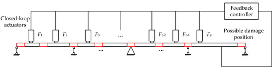
Figure 1.
A closed-loop system of a multispan structure.
In addition, to effectively excite the dynamic response of every span, we have to install actuators on most of the spans, which is not only costly, but also makes it difficult to implement the closed-loop dynamic load test in practice; hence, a single-gain scheme for closed-loop systems is not applicable for multispan structures.
For the above question, a multigain scheme is proposed in which each subsystem with a single gain is designed for each span. In this case, we only need to focus on the local structure rather than the whole structure, and only a few actuators installed on the target span can effectively enhance the sensitivity to the local damage of each span. A diagram of the single-gain subsystem designed for the target span of a multispan structure is shown in Figure 2. It is clear that only a minimum of two actuators can achieve the proposed multigain scheme, which is feasible in practice.
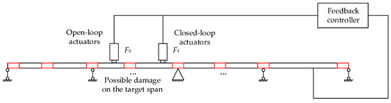
Figure 2.
A subsystem designed for the target span of a multispan structure.
Based on the above idea, for an n-span bridge structure, an n-gain closed-loop system can be designed by assigning n subsystems for each span, and then the gain set containing G1, G2, ……, and Gn can be obtained.
2.3. MSEBI Method for Damage Localization
There are lots of damage indicators that are sensitive to the local damage and are suitable for damage localization [36,37,38,39]. According to previous studies [40,41,42,43], the modal strain energy (MSE) index is quite effective in detecting structural damage, which is defined as the elemental stiffness matrix premultiplied and postmultiplied by the mode shape components together for every single element. For the i-th mode and j-th element, the undamaged and damaged elemental MSEs can be expressed as:
where and are MSEs of the i-th mode and the j-th element in undamaged and damaged status, respectively; and are the i-th mode shape in undamaged and damaged status, respectively; and the superscript “u” refers to “undamaged”, and “d” represents “damaged”. It is worth mentioning that the undamaged stiffness matrix is used in the approximate calculation of rather than since the actual damage condition is unknown.
It can be seen from the above equation that the rotational modes must be considered in the calculation; however, the angular displacement is difficult to measure in practice. To solve this problem, some methods are adopted, such as modal expansion, which will undoubtedly introduce extra errors into the calculation. In this case, a strain mode-based method is proposed to replace the displacement mode to improve the calculation accuracy since the strain modes are much easier to obtain without adding extra errors. Thus, the modified expressions of and are given as:
Using the new forms of and , the modal strain energy-based index (MSEBI) is expressed below:
where represents the MSEBI of the j-th element; m refers to the total number of modes; and n refers to the total number of elements.
It is clear that the values of MSEBI are closely related to the damage location and degree; in other words, the elements with larger values of MSEBI are potentially damaged, which can be used for preliminary damage location.
2.4. Hybrid ANN-PSO Algorithm for Damage Quantification
The ANN model is a nonlinear and adaptive information processing tool containing lots of interconnected analyzing units. It is developed on the basis of modern neuroscience investigation in order to process massive data by simulating the brain neural network. In the last few decades, research ANN has made great progress, which has overcome many complex practical problems in the research direction of intelligent robot, automatic control, forecast estimates, and many other academic disciplines, showing remarkable intelligence features. ANN has the ability of self-adaptation, self-organization, and self-learning; with the updated input information, the network can evolve and reconstruct for better data classification. In the ANN models, a neuron processing node can contain different objects, such as features, letters, or other meaningful abstract concepts. There are three main types of processing parts in the ANN model: input layer, output layer, and hidden layer, as displayed in Figure 3. Each part contains a large number of nodes connected to each other, and each node has a specific output function for the connected node in the previous part. Each connection between two nodes can be defined as the weight and bias, which can be used to process the output signals from the previous part and needs to be trained for a better classification effect.
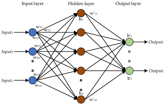
Figure 3.
Three-layer ANN architecture.
Figure 3 shows the basic framework of ANN modes. The inputs are imported into the input layer and transferred to the hidden layer through the connection. For the hidden layer, it can be regarded as a vital link between the input layer and the output layer. Each node in the hidden layer works as a data processing center and has multiple inputs and outputs, and the delivering messages are also processed on the connection based on training parameters (weight and bias). There are two basic data process modes, and the first one is displayed in Equation (25), representing the weighted summation process for the input signals from the last layer using the trained weight and bias.
where refers to the total input of the k-th node in the hidden layer; is the weight value of the connection between the i-th node in the input layer and k-th node in the hidden layer; is input information from the i-th node in the input layer; is the bias value of the k-th node in the hidden layer. Similarly, the data process for the connection between the hidden layer and output layer can be carried out.
Another data process mode is implemented after the summation, which can be considered as an activation function used to set a reasonable upper and lower bound value of the output. For different practical problems, a monotonically increasing linear or nonlinear function can be selected as the activation function, and, in this research, a sigmoid function is chosen to meet the nonlinear analysis requirements. In this manner, the outputs can be obtained as shown below:
where the outputj is the output signal of j-th node in the output layer, while the inputq is the input signal from the q-th node in the previous layer. The train parameters (weights and biases) are crucial in the ANN models, which determine recognition errors between the real and expected outputs and decide the success of the established network. However, due to the use of back propagation algorithm based on gradient descent, the neural network may find local minima rather than globe optima when the network is complex. To address this problem, the PSO algorithm is employed to find the optimized weights and biases in order to prevent the value from being trapped into local optimal.
The main idea of the PSO algorithm is to simulate the behavior of birds; in searching for the global optimal solution, each bird can be regarded as a particle with a memory function sharing function. In every search process, each particle can find one optimal solution (the local optimal) and determine the subsequent search direction and moving speed according to the overall optimal solution from the entire particles (the global optimal). Through the preset fitness function, the quality of the optimal solution can be judged, and the final global optimal solution can be found after several runs of the search process. Each particle of PSO is obtained using the updated iterative calculation in Equations (27) and (28). The first step is to update the location of each particle.
The second step is to update the velocity of each particle:
where and represent the location vector of i-th and i+1-th particles, respectively; refers the velocity vector of i+1-th particle; is the local optimal solution while represents the global optimal solution in this search process; and are two independent random numbers between 0 and 1; and are two learning factors which commonly take the equal values between 0 and 2; and w refers to the weight value. After several search process, the is compared and iteratively updated, and, using the fitness function, the final can be acquired.
In addition, in the process of damage detection using ANN, the objective fitness function needs to be constructed; here, the strain mode shapes of different closed-loop systems are chosen to build the objective function as shown below.
2.5. Flowchart of the Proposed Damage Diagnosis Approach
Following the above theory, the detailed process of the proposed damage diagnosis approach is outlined below, and the whole technological process is shown in Figure 4.
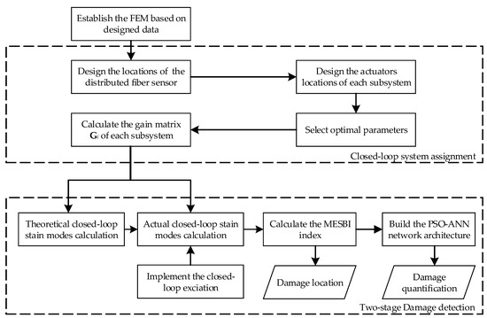
Figure 4.
Flowchart of the proposed two-stage damage diagnosis approach.
Step 1. Establish an accurate FEM based on the designed parameters and update the model with measured data if possible;
Step 2. Assign a multigain closed-loop system, including designing the locations of the distributed fiber sensor and actuators for each subsystem, selecting optimal assignment parameters and calculating the gain matrix Gi of each subsystem;
Step 3. Calculate the theoretical and actual closed-loop strain mode shapes before and after damage;
Step 4. Carry out the MSEBI method to approximately locate the damage;
Step 5. Build the PSO-ANN network architecture to quantify the damage degree.
3. Numerical Simulation
3.1. Brief Description of a Structural Example
To verify the validity of the proposed approach for the local microdamage of multispan structures, a two-span beam model, each with a span of 15 m + 15 m, is selected as a numerical example in this section. The beam model is simulated and divided into 30 elements using MATLAB, and the structural parameters are displayed in Table 1. To collect the dynamical strain responses, the distributed fiber sensor is simulated to be pasted at the bottom of the beam structure, and the dynamic strain data of the measured points are generated and acquired, as shown in Figure 5.

Table 1.
Structural parameters.

Figure 5.
A simple supported beam bridge structure.
First, the modal analysis for the open-loop (OL) system needs to be carried out, and the results show that the first three open-loop poles are located at , , and , which correspond to the first three bending modes. The third mode is a longitudinal vibration mode, and its pole lies at ; however, the fourth mode is selected instead because the horizontal force is difficult to apply to the structure to change the longitudinal mode shape.
3.2. Assignment of the Multiple Closed-Loop System
To assign the designed closed-loop system, four closed-loop excitation points (#5, #12, #20, and #27 nodes) and two open-loop excitation points (#9 and #23 nodes) n total are selected, as displayed in Figure 6. The closed-loop actuators are applied with feedback forces that are calculated in real time through a feedback controller, while the open-loop actuators are applied with Gaussian white noise with zero mean. In addition, the signal sampling frequency is 150 Hz.
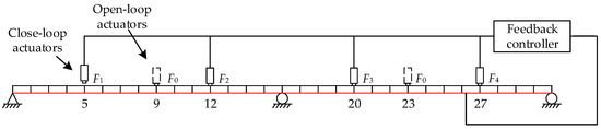
Figure 6.
Positions of the open-loop and closed-loop actuators.
Closed-loop actuators are adopted to assign the first three modes to enhance the sensitivity of strain mode shapes; thus, we need to focus on the sensitivity enhancement of these three modes to local damage. Based on the proposed multigain closed-loop scheme, a 2-gain, closed-loop system is designed according to the span number. For subsystem #1, the open-loop actuator is set on node #9, while closed-loop actuators are set on nodes #5 and #12; for subsystem #2, the open-loop actuator is set on node #23, while closed-loop actuators are set on nodes #20 and #27. In comparison, an open-loop system and a single-gain, closed-loop system are implemented to verify the effectiveness of the multigain approach. Both systems have an open-loop actuator at node #9, and the closed-loop actuator excitation points are located at nodes #5, #12, #20, and #27. As shown in Table 2, the designed information, including the excitation nodes and optimal designed variables, for each scheme system are obtained.
Table 2.
The position layout of actuators in different schemes.
As shown in Figure 7, we assign the first three poles of the bending modes in larger positions and move the neighboring poles closer to enhance the sensitivity of strain mode shapes to local damage. Specifically, the first three poles of the single-gain, closed-loop (SCL) system are located at , , ; for the subsystems of the multigain closed-loop (MCL) system, the closed-loop poles are assigned at , , and , , . Clearly, the SCL system can reach larger poles because it has more actuators to keep the system stable and robust.
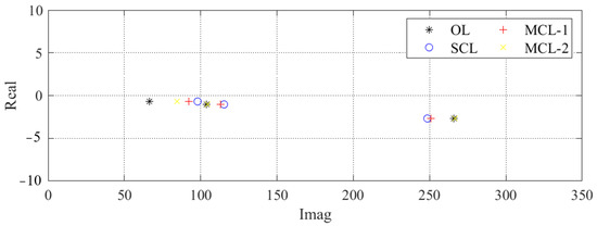
Figure 7.
Comparison of the pole positions of the open-loop and closed-loop systems.
3.3. Damage Cases
To verify the validity of the damage diagnosis approach in this study, considering that the closed-loop damage detection method aims at finding early damage, seven various damage conditions with minor stiffness reduction (by decreasing Young’s modulus) for various elements are simulated. The areas of potential damage are located at elements 1, 8, 15, and 23, as shown in Figure 8. The specific damage patterns include three single-element damage conditions, and three multielement damage conditions are displayed in Table 3.
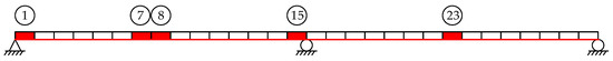
Figure 8.
Schematic of the damaged elements position.
Table 3.
Simulated damage conditions in the numerical study.
In engineering practice, the measured random noise caused by the environment and signal acquisition equipment will undoubtfully affect the measurement accuracy and interfere with the damage detection effectiveness; thus, the measured noise should be taken into consideration. In this paper, the identified strain mode shapes are mixed with Gaussian white noise, as shown below:
where is a closed-loop mode shape with noise; represents the noise level, and a noise level of 2% is considered in this paper; is a diagonal matrix with independent diagonal entries, which obey a normal distribution with a mean of 0 and variance of 1.
For each damage case, 200 simulated noise sets with a 2% noise level are generated and added to the identified open-loop and closed-loop strain mode shapes, and then the statistical results of the 200 sets of noise-polluted strain mode shapes (from open-loop and closed-loop systems) are calculated and compared.
3.4. Damage Diagnosis Results
3.4.1. Damage Localization Results
Based on the proposed MSEBI approach, we establish the MSEBI values using the strain mode shapes, and the damaged elements will have larger MSEBI values, with which we can preliminarily locate the damage. With the 2% noise-polluted strain mode shapes, the calculated damage localization indexes are displayed in Figure 9. The vertical bars with different colors refer to the average value of the 200 predictions obtained by the different methods, and the “T” marker line on the bars refers the standard deviation value of the 200 samples.
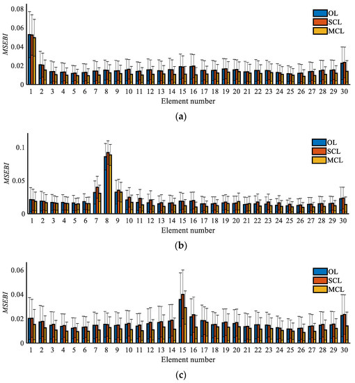
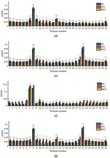
Figure 9.
Damage localization results based on the MSEBI method: (a) Case 1; (b) Case 2; (c) Case 3; (d) Case 4; (e) Case 5; (f) Case 6; (g) Case 7.
As seen in Figure 9, for most of the damage cases, the MSEBI indexes of those damaged elements are bigger than the healthy ones for all three systems, which indicates that the strain-based MSEBI has a good location effect. Meanwhile, the elements close to damaged ones also have relatively larger MSEBI values because the neighboring elements have shared nodes and because local damage can influence the nearby area. Therefore, the MSEBI values of the damaged elements and neighboring elements will appear to form a data peak. In addition, we can analyze the anti-noise performance according to the length of the “T” marker on top of the bars, and it is apparent that the results of the closed-loop systems have less interference than the open-loop systems, and the MCL system has the smallest standard deviation, which indicates that it has the best anti-noise performance. According to the previous simulation and analysis results, it is clear that the MSEBI values of the elements with more serious damage are relatively larger, and that the MSEBI values of the healthy elements are greater than 0 due to the global impact of local damage and noise interference.
Thus, the elements with a data peak of the MSEBI values are regarded as the possible damaged elements in this study, and the determination results are displayed in Table 4. We can see that all the systems have good location ability to find the actual damaged area. However, we must mention that the above results are obtained based on the statistical analysis for the 200 sets of noise-polluted data, which means that the identified results may have errors in a single independent test, and the identification accuracy will be strongly affected by the anti-noise performance of each system. Then, we can confirm that the closed-loop system is more stable in damage detection, while the MCL system can have better performance than the SCL system.
Table 4.
Determination of the damaged elements.
3.4.2. Damage Quantification Results
In this section, a hybrid ANN-PSO architecture with a three-layer network is applied, containing a 10-element hidden layer. The input data comprise the first three bending mode shapes, and the output data include damage locations and severities. In addition, by using the above damage location results, we can fix the output results on the target elements and assume that the remaining elements are all healthy without any stiffness reduction. To train the network for single damage cases, the stiffness of each element reduces from 20% to 0% with a step of 0.5%, while the rest of elements are healthy; then, 1200 data samples are created in total. Moreover, for multiple damage cases, we determined that the possible damaged elements are those numbered 8, 15, 23; thus, the conditions that each two elements are simultaneously damaged are added by the same damage simulation mode with the single damage cases, and about 4800 data samples are created in total. For the initial setup of PSO, while the two learning factors are c1 = 1.5 and c2 = 1.5, respectively, the weight value is 0.3. Then, the proposed hybrid ANN-PSO method is carried out, and the stop criteria of iteration are set as follows: the maximum iteration process number is 200 or the maximum tolerance limit of objective fitness function is smaller than 10−5, and the results are shown in Figure 10.
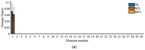
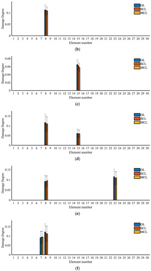
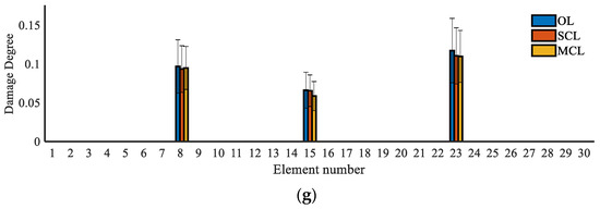
Figure 10.
Damage quantification results based on the hybrid ANN-PSO algorithm: (a) Case 1; (b) Case 2; (c) Case 3; (d) Case 4; (e) Case 5; (f) Case 6; (g) Case 7.
We can see that the damage degree can be accurately identified with all three systems; however, the closed-loop system has better accuracy and anti-noise performance due to higher sensitivity to damage. Specifically, the identified damage degrees and the error norm of the damage quantification results are shown in Table 5. In summary, the single-gain and multigain closed-loop systems both have a greater ability to detect the damage location and degree for all the damage conditions than the open-loop system through two-stage damage detection. In contrast, it can be further highlighted that the MCL systems are more effective in detecting local damage. Therefore, it is more practical to select the multigain closed-loop system, as it requires fewer actuators to implement.
Table 5.
Identified damage degree results.
3.4.3. Comparative Discussion with One-Stage Damage Diagnosis Using Sensitivity Matrix
Different from the two-stage damage diagnosis approach, the damage degree is obtained directly based on the sensitivity-based method using the relationship between the changes in the measured strain mode shapes and the variation in the structure parameters, as shown below:
where is the sensitivity matrix of the closed-loop strain mode shapes.
Then, the structural parameter changes can be obtained by the reversion method,
where denotes the pseudoinverse of the matrix .
Using Equation (32), the damage detection results of the multigain closed-loop system are obtained, and the comparison results with the two-stage method are exhibited in Figure 11. As seen, for the damaged elements, the two-stage method has better accuracy with an error norm of less than 1.5, and the healthy elements appear to have no stiffness reduction, while the one-stage method inevitably produces a misjudgment and detection error. The test results clearly indicate that the two-stage approach has a better effect. Moreover, regarding CPU time, taking the single damage condition as an example, the one-stage and two-stage damage detection methods take approximately 13 s and 47 s, respectively, which means that the one stage method is faster but both methods have quick computational efficiency.
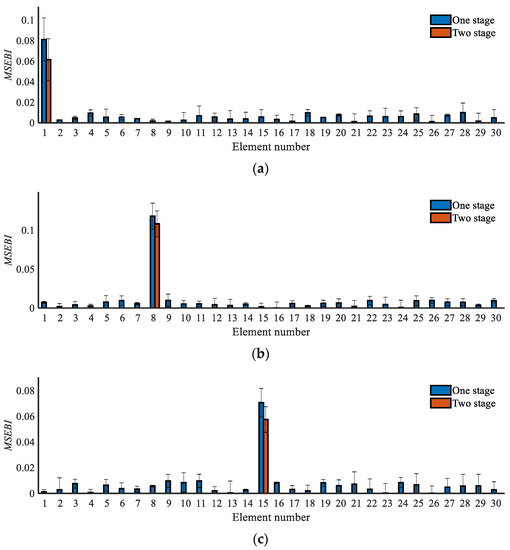
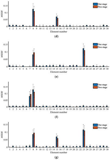
Figure 11.
Comparison results between the one-stage and two-stage damage detection methods: (a) Case 1; (b) Case 2; (c) Case 3; (d) Case 4; (e) Case 5; (f) Case 6; (g) Case 7.
3.4.4. Comparative Discussion with the ANN-Only Algorithm for Damage Quantification
Last, a comparison between the ANN-PSO and ANN-only algorithms is carried out. For the ANN, the backpropagation-based L–M algorithm is employed. The comparison results between the two methods are exhibited in Figure 12.
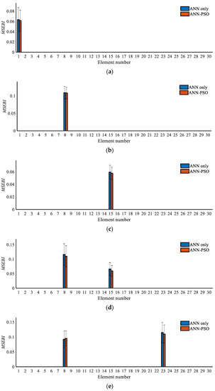
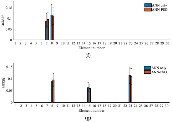
Figure 12.
Comparison results between the ANN-only and ANN-PSO algorithms: (a) Case 1; (b) Case 2; (c) Case 3; (d) Case 4; (e) Case 5; (f) Case 6; (g) Case 7.
As seen in the figures, for the single damage cases, both the ANN-PSO and ANN-only algorithms have good damage degree detection accuracy, and, to be more specific, the former has less detection error. Moreover, for the multiple damage cases, the ANN-only algorithm may obtain less accurate results while the ANN-PSO algorithm still has a good effect. The results indicate that the ANN algorithm can only accurately determine the damage degree of data samples that are part of the trained network, and the underlying cause lies in the fact that the ANN algorithm can easily become trapped in local minima.
In addition, to verify the validity of the ANN structure, one of the learning coefficients (R) and fitness tolerances in single damage cases are shown in Figure 13 and Figure 14.
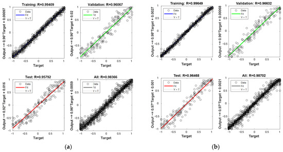
Figure 13.
Regression of the training process for the simulated example—single damage: (a) ANN-PSO; (b) ANN-only.
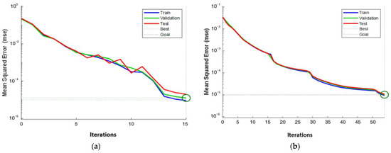
Figure 14.
Fitness tolerance for the simulated example—single damage: (a) ANN-PSO; (b) ANN-only.
Figure 13 shows the regression of the training process, which indicates the difference errors between the expected outputs and the real outputs for training, validation, and testing. We can see that the data trend lies along the 45-degree line, and both regressions of the ANN-PSO and ANN-only methods are larger than 0.96 for the whole damage cases, all of which demonstrate a good training effect.
As shown in Figure 14, the ANN-PSO and ANN reach the global optimal for convergence at about 15 and 54 iteration steps, respectively. Moreover, regarding CPU time, the ANN-PSO and ANN-only damage detection methods take 47 s and 28 s, respectively. In summary, the ANN-PSO is undoubtedly superior to the ANN in detection accuracy and convergence iterations; however, the computation speed of ANN is faster. In contrast, the former algorithm can lead to a superior performance and reach a balance between the speed of convergence and identification accuracy, making it a better choice for detecting damage exactly.
4. Concluding Remarks
In this paper, a two-stage approach for damage diagnosis is proposed, combining the MSEBI method with a hybrid ANN-PSO algorithm based on the fully distributed strain mode of a structure under multigain feedback control. According to the theoretical analysis and numerical simulation, the following conclusions are drawn:
- (i)
- A multigain closed-loop system is established to improve the sensitivity of strain mode shapes for structural damage in different spans, with which the MSEBI method and hybrid ANN-PSO algorithm are proposed to locate and quantify the small damage of the multispan structure, and the performance of the proposed method is validated through a numerical example of a two-span beam structure;
- (ii)
- The MCL system performs more effectively than the OL and SCL systems for detecting local damage, while the MCL system requires fewer actuators than the SCL system, making it more economical and practical for structure testing;
- (iii)
- Compared with the one-stage, sensitivity-based damage detection approach, the two-stage method has a better effect and accuracy, which can help avoid misjudgment for undamaged elements and realize fast damage detection;
- (iv)
- The hybrid PSO-ANN algorithm has a better detection effect, while the ANN-only algorithm may easily become trapped in local minima and become less accurate;
- (v)
- The proposed closed-loop damage diagnosis method is carried out in real time online, which is difficult to implement in practice; thus, further research on method implementation based on virtual output feedback should be investigated in the future.
Author Contributions
All authors discussed and agreed upon the idea and made scientific contributions. Z.Z. wrote the theoretical part, abstract and conclusion parts; K.D. and Z.F. wrote the numerical example part; Y.L. wrote the introduction part and revised the paper. All authors have read and agreed to the published version of the manuscript.
Funding
This study is supported by the Heilongjiang Provincial Key Research & Development Program (Grant No: GA21A303).
Institutional Review Board Statement
Not applicable.
Informed Consent Statement
Not applicable.
Data Availability Statement
Not applicable.
Conflicts of Interest
The authors declare that they have no known competing financial interests or personal relationships that could have appeared to influence the work reported in this paper.
References
- Ellingwood, B.R. Risk-informed condition assessment of civil infrastructure: State of practice and research issues. Struct. Infrastruct. Eng. 2005, 1, 7–18. [Google Scholar] [CrossRef]
- Frangopol, D.M.; Liu, M. Maintenance and management of civil infrastructure based on condition, safety, optimization, and life-cycle cost. Struct. Infrastruct. Eng. 2007, 3, 29–41. [Google Scholar] [CrossRef]
- Frangopol, D.M.; Saydam, D.; Kim, S. Maintenance, management, life-cycle design and performance of structures and infrastructures: A brief review. Struct. Infrastruct. Eng. 2012, 8, 1–25. [Google Scholar] [CrossRef]
- Kim, J.M.; Son, K.; Yoo, Y.; Lee, D.; Kim, D.Y. Identifying risk indicators of building damage due to typhoons: Focusing on cases of south Korea. Sustainability 2018, 10, 3947. [Google Scholar] [CrossRef]
- Sony, S.; Laventure, S.; Sadhu, A. A literature review of next-generation smart sensing technology in structural health monitoring. Struct. Control Health Monit. 2019, 26, e2321.1–e2321.22. [Google Scholar] [CrossRef]
- Mishraa, M.; Lourençob, P.B.; Ramana, G.V. Structural health monitoring of civil engineering structures by using the internet of things: A review. J. Build. Eng. 2021, 48, 103954. [Google Scholar] [CrossRef]
- Amezquita-Sanchez, J.P.; Adeli, H. Signal Processing Techniques for Vibration-Based Health Monitoring of Smart Structures. Arch. Comput. Methods Eng. 2016, 23, 1–15. [Google Scholar] [CrossRef]
- Mishra, M. Machine learning techniques for structural health monitoring of heritage buildings: A state-of-the-art review and case studies. J. Cult. Herit. 2021, 47, 227–245. [Google Scholar] [CrossRef]
- Lian, J.J.; Cai, O.; Dong, X.F.; Jiang, Q.; Zhao, Y. Health monitoring and safety evaluation of the offshore wind turbine structure: A review and discussion of future development. Sustainability 2019, 11, 494. [Google Scholar] [CrossRef]
- Abdeljaber, O.; Avci, O.; Kiranyaz, S.; Gabbouj, M.; Inman, D.J. Real-time vibration-based structural damage detection using one-dimensional convolutional neural networks. J. Sound Vib. 2017, 388, 154–170. [Google Scholar] [CrossRef]
- Zhang, Y.; Miyamori, Y.; Mikami, S.; Saito, T. Vibration-based structural state identification by a 1-dimensional convolutional neural network. Comput.-Aided Civ. Infrastruct. Eng. 2019, 34, 822–839. [Google Scholar] [CrossRef]
- Fan, W.; Qiao, P. Vibration-based Damage Identification Methods: A Review and Comparative Study. Struct. Health Monit. 2011, 9, 83–111. [Google Scholar] [CrossRef]
- Zhu, D.; Yi, X.; Wang, Y. A local excitation and measurement approach for decentralized damage detection using transmissibility functions. Struct. Control. Health 2016, 23, 487–502. [Google Scholar] [CrossRef]
- Ray, L.R.; Tian, L. Damage detection in smart structures through sensitivity enhancing feedback control. J. Sound Vib. 1999, 227, 987–1002. [Google Scholar] [CrossRef]
- Koh, B.H. Damage Identification in Smart Structures Through Sensitivity Enhancing Control. Master’s Thesis, Thayer School of Engineering, Dartmouth College, Hanover, NH, USA, 2003. [Google Scholar]
- Koh, B.H.; Ray, L.R. Feedback controller design for sensitivity based damage localization. J. Sound Vib. 2004, 273, 317–335. [Google Scholar] [CrossRef]
- Ray, L.R.; Koh, B.H.; Tian, L. Damage detection and vibration control in smart plates: Towards multifunctional smart structures. J. Intell. Mater. Syst. Struct. 2000, 11, 725–739. [Google Scholar] [CrossRef]
- Koh, B.H.; Ray, L.R. Localization of damage in smart structures through sensitivity enhancing feedback control. Mech. Syst. Signal Process. 2003, 17, 837–855. [Google Scholar] [CrossRef]
- Ray, L.R.; Marin, I.S. Optimization of control laws for damage detection in smart structures. In Proceedings of the SPIE-the International Society for Optical Engineering, San Jose, CA, USA, 25–28 January 2000; Volume 3984, pp. 395–402. [Google Scholar]
- Solbeck, J.A.; Ray, L.R. Damage identification using sensitivity-enhancing control and identified models. J. Vib. Acoust. Trans. ASME 2006, 128, 210–220. [Google Scholar] [CrossRef]
- Jiang, L.J.; Tang, J.; Wang, K.W. An Optimal Sensitivity-Enhancing Feedback Control Approach via Eigenstructure Assignment for Structural Damage Identification. J. Vib. Acoust. 2007, 129, 771–783. [Google Scholar] [CrossRef]
- Jiang, L.J.; Wang, K.W. An experiment-based frequency sensitivity enhancing control approach for structural damage detection. Smart Mater. Struct. 2009, 18, 065005. [Google Scholar] [CrossRef]
- Bernal, D. Eigenvalue sensitivity of sampled time systems operating in closed loop. Mech. Syst. Signal Process. 2018, 105, 481–487. [Google Scholar] [CrossRef]
- Bernal, D. State observers in the design of eigenstructures for enhanced sensitivity. Mech. Syst. Signal Process. 2018, 110, 122–129. [Google Scholar] [CrossRef]
- Bernal, D.; Ulriksen, M.D. Output feedback in the design of eigenstructures for enhanced sensitivity. Mech. Syst. Signal Process. 2018, 112, 22–30. [Google Scholar] [CrossRef]
- Masoudi, A.; Belal, M.; Newson, T.P. A distributed optical fibre dynamic strain sensor based on phase-OTDR. Meas. Sci. Technol. 2013, 24, 085204. [Google Scholar] [CrossRef]
- Soto, M.A.; Thévenaz, L. Modeling and evaluating the performance of Brillouin distributed optical fiber sensors. Opt. Express 2013, 21, 31347–31366. [Google Scholar] [CrossRef]
- Castillo-Mingorance, J.M.; Sol-Sánchez, M.; Moreno-Navarro, F.; Rubio-Gámez, M.C. A Critical Review of Sensors for the Continuous Monitoring of Smart and Sustainable Railway Infrastructures. Sustainability 2020, 12, 9428. [Google Scholar] [CrossRef]
- Glisic, B.; Hubbell, D.; Sigurdardottir, D.; Yao, Y. Damage detection and characterization using long-gauge and distributed fiber optic sensors. Opt. Eng. 2013, 52, 087101. [Google Scholar] [CrossRef]
- Hoult, N.A.; Ekim, O.; Regier, R. Damage/Deterioration Detection for Steel Structures Using Distributed Fiber Optic Strain Sensors. J. Eng. Mech. 2014, 140, 04014097. [Google Scholar] [CrossRef]
- Gu, J.; Gul, M.; Wu, X. Damage detection under varying temperature using artificial neural networks. Struct. Control Health 2017, 24, e1998. [Google Scholar] [CrossRef]
- Cha, Y.J.; Choi, W.; Büyüköztürk, O. Deep Learning-Based Crack Damage Detection Using Convolutional Neural Networks. Comput-Aided Civ. Inf. 2017, 32, 361–378. [Google Scholar] [CrossRef]
- Khodabandehlou, H.; Pekcan, G.; Fadali, M.S. Vibration-based structural condition assessment using convolution neural networks. Struct. Control Health 2019, 26, e2308. [Google Scholar] [CrossRef]
- Khatir, S.; Boutchicha, D.; Thanh, C.L.; Tran-Ngoc, H.; Nguyen, T.N.; Abdel-Wahab, M. Improved ANN technique combined with Jaya algorithm for crack identification in plates using XIGA and experimental analysis. Theor. Appl. Fract. Mech. 2020, 107, 102554. [Google Scholar] [CrossRef]
- Mishra, M.; Barman, S.K.; Maity, D.; Maiti, D.K. Performance Studies of 10 Metaheuristic Techniques in Determination of Damages for Large-Scale Spatial Trusses from Changes in Vibration Responses. J. Comput. Civ. Eng. 2020, 34, 04019052. [Google Scholar] [CrossRef]
- Barman, S.K.; Mishra, M.; Maiti, D.K.; Maity, D. Vibration-based damage detection of structures employing Bayesian data fusion coupled with TLBO optimization algorithm. Struct. Multidiscip. Optim. 2021, 64, 2243–2266. [Google Scholar] [CrossRef]
- Wang, S.Q.; Liu, F.S.; Zhang, M. Modal Strain Energy Based Structural Damage Localization for Offshore Platform using Simulated and Measured Data. J. Ocean Univ. China 2014, 13, 397–406. [Google Scholar] [CrossRef]
- Zhang, J.; Li, P.J.; Wu, Z.S. A new flexibility-based damage index for structural damage detection. Smart Mater. Struct. 2013, 22, 025037. [Google Scholar] [CrossRef]
- Naderi, A.; Sohrabi, M.R.; Ghasemi, M.R.; Dizangian, B. A swift technique for damage detection of determinate truss structures (2). Eng. Comput. 2021, 38 (Suppl. 2), 1427–1436. [Google Scholar] [CrossRef]
- Seyedpoor, S.M.A. Two stage method for structural damage detection using a modal strain energy based index and particle swarm optimization. Int. J. Non-Linear Mech. 2012, 47, 1–8. [Google Scholar] [CrossRef]
- Shi, Z.Y.; Law, S.S.; Zhang, L.M. Structural damage localization from modal strain energy change. J. Sound Vib. 1998, 218, 825–844. [Google Scholar] [CrossRef]
- Shi, Z.Y.; Law, S.S.; Zhang, L.M. Improved damage quantification from elemental modal strain energy change. J. Eng. Mech.-ASCE 2002, 128, 521–529. [Google Scholar] [CrossRef]
- Wu, S.Q.; Zhou, J.X.; Rui, S.; Fei, Q.G. Reformulation of elemental modal strain energy method based on strain modes for structural damage detection. Adv. Struct. Eng. 2017, 20, 896–905. [Google Scholar] [CrossRef]
Publisher’s Note: MDPI stays neutral with regard to jurisdictional claims in published maps and institutional affiliations. |
© 2022 by the authors. Licensee MDPI, Basel, Switzerland. This article is an open access article distributed under the terms and conditions of the Creative Commons Attribution (CC BY) license (https://creativecommons.org/licenses/by/4.0/).